Rev. bras. oceanogr., 47(1):11-27, 1999
Environmental forcing on phytoplankton biomass and primary
productivity of the coastal ecosystem in
Ubatuba region, southern Brazil
Salvador Airton Gaetal,2, Sylvia Maria Susini Ribeiro1,
Patricia Mercedes Metzler2, Maria Solange Francos & Donato Seiji Abe3
lInstituto Oceanográfico da Universidade de São Paulo (Caixa Postal 66149, 05315-970 São Paulo, SP, Brasil)
2Fundação de Estudos e Pesquisas Aquáticas - FUNDESP A (Av. Caxingui, 160,05579-000 São Paulo, SP, Brasil)
3Instituto Internacional de Ecologia - IIE (Caixa Postal 694, 13560-460 São Carlos, SP, Brasil)
.
Abstract:A time series of chlorophylIaand.insituprimary production sampled over a period of 33 daysduring summerin Ubatuba region,southeastemBrazil, was subjectedto multivariateand hannonic analysis. Principal Component Analysis has revealed four factors interpreted as (i) South Atlantic Central Water forcing;(ii) Transientfrontalsystemsand rain falIforcings;(iii) Wind forcingnormalto the coast; (iv) Wind forcing paralIel to the coast, as main factors in the variability of the phytoplanktonbiomass and primary productivity.Splitting of the time series accordingto four main events which had profound effects on the physicochemicalcharacteristicsof the region showed the folIowingvariations in the primary productivity integratedover the photic layer (g C m,2day,I):mixing~stratification period,0.401 0.11; heavy rainfall, 1.2410.28; stratificationafterrainfall,0.74 1 0.10; stratification~mixing period,0.90 1 0.27; stratification after deep mixing, 0.63 1 0.28. Harmonicanalysis revealedtwo indistinguishablesignificantpeaks ofthe
phytoplankton biomass
-
one at a period of 8.25 days and one at a period of 6.6 days, contributing, respectively, about 17 and 32% ofthe total variance. Atmospheric forcing showed a characteristic periodof 200-264 hours while phytoplankton biomass response ranged over the 144-192 hours time scales and primary productivity was best related to the environment 360 hours before. Relative to total nitrogenand biomass primary productivity oscillations were lagged about 96-144 hours. 'lhe interruption of steady-state conditions by transient atmospheric ev~nts and wind field intensification are the determining factors driving phytoplankton changes in this coastal enviromnent..
Resumo: Uma série temporalde clorofilaae produçãoprimáriaobtida em um períodode 33 dias durante o verão na região de Ubatuba, sudeste do Brasil, foi submetida à análise multivariada e hannônica. A Análise de Componentes Principais revelou quatro fatores interpretados como (i) Água Central do Atlântico Sul; (ii) Sistemas frontais transientes e chuvas; (iii) Ventos normais à costa; (iv) Ventos paralelos à costa. Estes fatores atuam como forçantes ambientais na determinação da variabilidade observada na biomassa fitoplanctônica e produtividade primária. A divisão da série temporal de acordo com quatro eventos modificadores das características fisicoquímicas da região mostrou a seguinte variabilidade na produção primária integrada (g C m,2 dia,l) na camada eufótica: coluna de água homogênea em processo de estratificação térmica- 0,4010,11; coluna de água estratificada e chuvas intensas- 1,2410,28; coluna de água misturada em fase de estratificação térmica após intensas chuvas- 0,7410,10; coluna de águaestratificada em fase de processo de mistura- 0,9010,27; coluna de água homogênea em fase de estratiflcação térmica após intensa mistura- 0,6310,28. A Análise Harmônica revelou dois picos de biomassa significativos- um com período de 8,25 dias e outro com período de 6,6 dias, contribuindo, respectivamente, com 17 e 32% da variância total da série. A forçante atmosférica apresentou um período característico de 200-264 horas enquanto que a escala de resposta da biomassa fitoplanctônica variou de 144-192 horas e a de produtividade primária um período de 360 horas. Em relação à biomassa e nitrogênio total, a produtividade primária apresentou uma defasagem de 96-144 horas..
Descriptors: Chlorophyll a,Primary productivity, Time series, Ubatuba coastal waters.Introduction
According to Margalef (1978), the input of external turbulent energy in the water column acts as
the supplementary energy to the plankton
communities. This is the case in shallow and ftequently disturbed systems where wind is the main source of kinetic energy generating water exchanges between the shelf and the coast (Castro Filho et ai.,
1987).
The Ubatuba region on the northern coast of São Paulo State-Brazil has been studied with relation to the phytoplankton and the primary production specially in coastal stations (Kutner, 1961; Tundisi
et ai.,1978; Sassi, 1978; Kutner & Sassi, 1979; Sassi
& Kutner, 1982; Oliveira, 1980; Teixeira & Tundisi, 1981; Teixeira, 1973; 1979; 1980; Perazza, 1982; Teixeira & Gaeta, 1990; Gaeta et ai., 1990); and in
the shelf by Soares (1983) and Susini-Zilmanri (1990). Available data on environmental forcing in this region is restricted to surface sampling at a fixed station inside the Flamengo Bay, a well protected environment under the peculiar hydrodynamic mechanisms ofvery shallow waters (Teixeira, 1986). We hypothesize that wind and other environmental forces are significant factors in phytoplankton productivity and biomass accumulation in this region.
In summer 1988, we followed
phytoplankton and in situ primary production
dynamics in the coastal inshore waters of Ubatuba region. The time series of Chlorophyll a, Primary
Production and associated environmental variables are presented. The results of multivariate and harmonic analysis ofthese series are discussed.
Materiais and methods
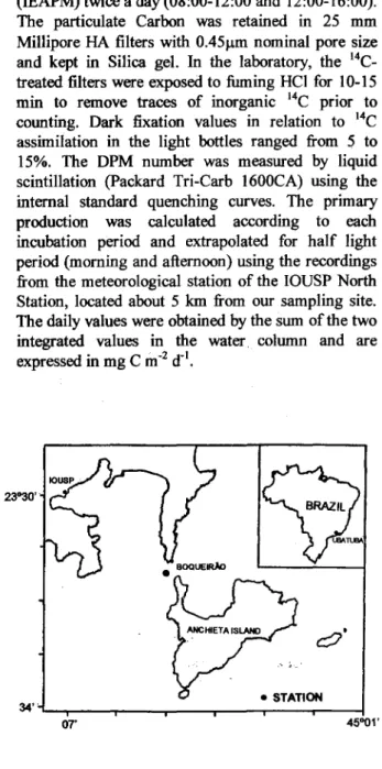
The sampling station was located in the coastal zone at,Boqueirão near Anchieta Island on the north coast of the São Paulo State, Brazil (Fig. 1). This sampling station was occupied for 33 consecutive days, between 12 February and 15 March 1988. Water samples were collected with 5 L Van Dom bottles at five depths corresponding to the light extinction percentages of 100, 50, 25, 10 and 1%, obtained with the Secchi disc, at 6:00, 12:00 and
18:00 h (local time).
Primary production was determined in situ
with subsamples collected at 6:00 and 12:00 h and kept horizontally in the water column at the original depths. A system of stainless steel ftames attached to the hydrographic wire with a weight of 7 kg and a buoy was tied to the boat at a distance long enough to prevent shading. The subsamples (60-85 ml) were
incubated ftom 4 to 6 h with two transparent bottles and one dark bottle with 10 J.l.Ci Na HI4C03 (IEAPM) twice a day (08:00-12:00 and 12:00-16:00). The particulate Carbon was retained in 25 mm Millipore HA filters with 0.45J.1.mnominal pore size and kept in Silica gel. In the laboratory, the 14C_ treated filters were exposed to fuming HCI for 10-15 min to remove traces of inorganic 14C prior to counting. Dark fixation values in relation to 14C assimilation in the light bottles ranged ftom 5 to 15%. The DPM number was measured by liquid scintillation (packard Tri-Carb 1600CA) using the internal standard quenching curves. The primary production was calculated according to each incubation period and extrapolated for half light period (moming and aftemoon) using the recordings ftom the meteorological station of the IOUSP North Station, located about 5 km ftom our sampling site. The daily values were obtained by the sum of the two integrated values in the water, column and are expressed in mg C m-2d-I.
CJ'
34'-07' 45"01'
Fig. 1. Map showing the location ofthe sampling station.
The phytoplankton biomass was retained in Whatman GF/F filters and estimated by Chlorophyll
a (mg Chl a m-3) after extraction in 90% acetone
using the trichromatic equations of Jeffrey &
Humphrey (1975); and pheopigments using
Lorenzen and Jeffrey (1980). The nutrients were determinated following Grasshoffet aI., 1983 (N03-,
N02-, PO/,' and Si(OH)4) and Aminot &
Chaussepied, 1983~ +) in the filteredsea water.
GAETA el aI.: Environrnental forcing on phytoplankton and primary productivity 13
The temperature was measured with
reversible thermometers using Nansen bottles at fixed depths (O, 5, 10, 20 and 30 m) and corrected with their own calibration curves. The salinity was measured with an induction salinometer (Beckman RS-7C) after frequent calibration with normal water and using the Practical Salinity Scale of UNESCO (1981a).
The sea water density (cr t) was calculated by the International State Equation (UNESCO, 1981b). Estimation of the differences in the vertical gradients of in situ density was obtained
by means of graphic interpolation, taking into account the recommendations of Millard et ai.
(1990). The mixed layer extended from surface until the depth at which the vertical gradient of density started continuously. The water column stability was estimated through ~T (temperature difference between surface, Zo, and bottom of tbe euphotic zone, z,,) and ~ crt(crt Zo
-
crtz,,).Also theeuphotic zone : mixing layer ratio (z":z,,,) was estimated.
The meteorological data of global solar radiation (Cal cm'2 h'l) and rain fall (mm), measured at the Ubatuba Station were collected by the IOUSP Physical Oceanography Department -Meteorology Laboratory and expressed as W m'2 6 h'l (1/2 photoperiod, morning and afternoon) and mm 12 h-I
before sampling. Wind speed and direction,
registered at the Moela Island (24°03'S 46°16'W) were obtained :fi:om DHN-Brazilian Navy and expressed as degrees and m S'I,respectively.
The data were reduced to a rectangular matrix of environmental parameter values versus sampling periods. For Principal Component Analysis
(PCA) analysis a matrix of product-moment
correlation coefficients was calculated :fi:om the standardized data (Draper & Smith, 1966; Legendre & Legendre, 1984a; 1984b) and the first four
eigenvectors were extracted along with the
corresponding eigenvalues for each plot.
AlI time series were expressed in a common sample period of 12 hours. The time series were subjected to Harmonic Analysis (Jenkins & Watts, 1968). This statistical operation may be regarded as an analysis of variance in which the total variance of a variable or property fluctuation is partitioned into contributions arising :fi:omprocesses with different characteristic time scales (platt & Denman, 1975). Thus, harmonic analysis of a record of observations results in a sorting of total variance of the record into its component :fi:equencies. The harmonic results presented in this paper were computed with a fast Fourier transform algorithm. The number of sampling observations was 66 with a sampling interval of 12 h (33 harmonics). Critical values of
the periodograms were estimated as by Anderson (1971).
Results
Chlorophyll a, total dissoived inorganic nitrogen,
pheopigments and primary production:
distribution and variability.
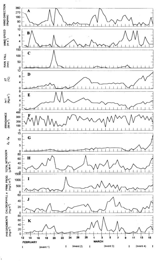
Chlorophyll a distribution (Fig. 2A) was
shifted for values up to 10.0 mg m,2, showing the average value of 16.2, standard deviation of 11.2 and error (estimated by the quotient between the confidence interval for 90% and two times the parametric average) of 114%. Practically 70% ofthe observations were between 1.5 and 20.0 and the highest value (53.3 mg m'2) occurred at Mar. 6th (Fig. 3J) after a 6 day period of prevailing winds (Figs 3A and 3B) that favored the turbulence and mixing processes (Figs 3D and 3E). Three other peaks can be seen in Fig. 3J: between Feb. 18th and 19th,Feb. 28thand 29thand at Mar. 15th.The last two occurred at the thermal stratification period (Fig. 3D, Feb. 23rd to 28th and Mar. 10th to 15th) with the presence and evolution of a pycnocline (Fig. 3E, Feb. 23rd to 27th and Mar. 10thto 15th,respectively). At these two periods, the prevailing winds were from the first quadrant (Fig. 3B) and the intensities were :fi:om2 to 7 m S'I (Fig. 3A). The first peak of the series occurred between Feb. 18th_and19thand can be associated to a progressive stratification process period (Fig. 3D and 3E, Feb 12th to 19th). At this period one can see the prevailing winds, at low to moderate strength (Fig. 3B), from the first quadrant (Fig. 3A) before the chlorophyllapeak.
Total dissolved inorganic nitrogen (Fig. 2B) showed an average value of28.3 mM N m,2, s.d. 16.0 and a range from 9.6 to 75.3. About 85% of the observations fell between 9.6 and 37.9 mM N m'2. In general, nitrogen changes (Fig. 3H) roughly followed those observed in ~ T (Fig. 3D). Data suggest a relationship between thermal stratification processes and nitrogen with coinciding peaks; the exceptions were at Mar. 4th, 6th,
~
and 11th,which could beassociated to turbulence and rainfall periods.
Pheopigments (Fig. 2C) showed 71% of the values between 0.5 and 22.0 mg m'2, with an average of 17.1, s.d. 15.5 and an error of 151%. In the time series (Fig. 3K), the first two peaks between Feb. 17th and 18thand Feb. 19thto 20th appeared to be related to the modifYing events ofthe water column (Fig. 3D and 3E) and to the nitrogen availability (Fig. 3H), the latter with continental mn off contribution (Fig.
3C). Between Feb. 29th and Mar. 3rd, three
chlorophyll a trough at the same time, suggest to
indicate active grazing processoIt is worth noting the wind direction change (3rdand 4thquadrant; Fig. 3A) and the water column mixing (Fig. 3D and 3E).
Primary production (Fig. 2D) showed an average value (mg C m-26 h-I) 352.4, s.d. 202.0 and tbe error 100%. About 71% ofthe observations were between 80.3 and 355.3 and one observation was higher than 1,000 three days aftera rain fall peak (Fig. 3C).
Multivariate analysis
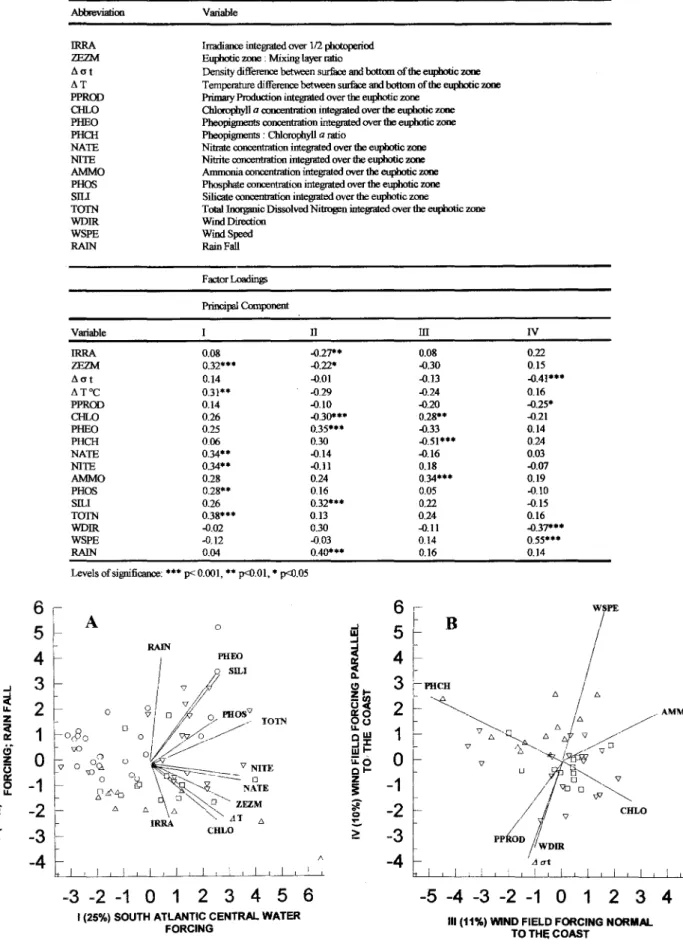
Table 1 shows the variables and the tespective abbreviations for the PCA and the
significance levels of the factor loadings
(correlations between the variables and the principal components). Results showed four components explaining, respective1y, 26, 14, 11 and 10% of the total variance of the data. Figure 4A shows the first two components. The first component is composed by the nutrients (TOTN 0.38***; NATE 0.34***;NITE 0.34***; PHOS 0.28**), the ratio euphotic zone: mixing layer (ZEZM 0.32***) and the thermal gradient (Li T 0.31**). The second component, explaining 14% ofvariance, is composed by rain fall (RAlN 0.40***), pheopigments (PHEO 0.35*** and Silicate (SILI 0.32***) opposing the phytoplankton biomass (CHLO -0.30***), the total solar irradiation (IRRA -0.27**) and the light availability in the mixing zone (ZEZM -0.22*).
Fig. 2. Frequency distributions (n=66): (A) Chlorophyll a ; (B) Total inorganic dissolved
nitrogen; (C) Pheopigments; (D) Primary production.
20l 20
A
"1
B-]
']
<IJ
5J
z
O
5
:>
f;riI
!
o 1""1,. Ir ,. I' '[v '; v r r I' rI ' 1",. r 'IA I oO o 10
20 30 40 50 60 o 20 40 60 80 100
O ....
mg Chl a'. m-2 mM Nt m-2
h1
:
;..J
g
C
25 l7"7l7'71
D
20l 15
15
10 10
5 5
o
I,. ( .,
í
....,. ( " ,. 111,. " ,. (I' fI Ir ,. 1 oo 20 40 60 80 o 250 500 750 1000 1250 1500
GAETAet aI.:Environmental forcing on phytoplankton and primary productivity 15
D
E
G
O 80 80
40
20
O
J I ! I I I t I
12 14 16 18 20 22 24 26 FEBRUARY
1 3
MARCH
5 7 9 11 13 15
(event 1) (event 2) (event 3) (event4)
Fig. 3. Time series ofphysical, chemical and biological variables.
z o
i= 360
ü
w 270
Q;;-e'"'" 180 e
z'" 90 O
e 12
w w
a.. a
C/)
e-z'", 4 E
o 150
....J
....J 100
«u.
z- 50
O
12
1-0 8
<1"--4
O 8
_ E 64
2
w O
ü 400
Z 300
«
CN-'E 200 Q;; 100 o 15
10
5 z
o a: I-Z ....J' «E b=< 1-3 ci
-a.. E
::;!ü
.[ '"
....J
J:
a.. -OE
ü_
f!! z w =<
C)
ã:f'f-OE W'"
AbbreviaIion Variable
Table 1. Principal component analysis: variables and factor loadings.'
IRRA ZEZM liat liT PPROD CHLO PHEO PHCH NATE NITE AMMO PHOS
Slll
TOTN WDIR WSPE RAIN
1rradianre integrated over 1/2 photoperiod Eupbotic zone : Mixing layer rntio
Density difference bemren surfure and bottom of the euphotic zone
Temperature difference bemren surfure and bottom of the euphotic zone
Primmy Production integrated over the euphotic zone
Chloropbyll aconcentration integrated over the euphotic zone
Pheopigments concentrntion integrated over the euphotic zone
Pheopigments : Chlorophyll arntio
Nitrate concentrntion integrated over the euphotic zone Nitrite concentration integrated over the euphotic zone Arnrnonia concentration integrated over the euphotic zone Phosphate concentrntion integrated over the euphotic zone Silicate concentration integrated over the euphotic zone
ToIallooI!>lmic Dissolved Nitrogen integrated over the euphotic zone Wind Direction
Wind Speed Rain Fall
F actor Loa<Iing;
Principal Component
IRRA ZEZM 8a t liToC PPROD CHLO PHEO PHCH NATE NITE AMMO PHOS Slll TOTN WDIR WSPE RAIN Variable
Levels ofsignificanre: *** p< 0.001, ** p<O.OI, * p<O.05
1(25%) SOUTH ATLANTIC CENTRAL WATER
FORCING III (11%) WlND FIELD FORCING NORMAL
TO THE COAST
Fig. 4. Principal component analysis: (A) First x Second component; (B) Third x Fourth component. (o Period 1- Feb. 12-23; D Period 2- Feb. 24-29; V Period 3 Mar. 01-09; 11Period 4 Mar. 10-15).
TI m IV
0.08 -0.27** 0.08 0.22
0.32*" -0.22* -0.30 0.15
0.14 -0.01 -0.13 -0.41***
0.31** -0.29 -0.24 0.16
0.14 -0.10 -0.20 -0.25*
0.26 -0.30*** 0.28** -0.21
0.25 0.35*** -0.33 0.14
0.06 0.30 -0.51*** 0.24
0.34** -0.14 -0.16 0.03
0.34** -0.11 0.18 -0.07
0.28 0.24 0.34*** 0.19
0.28** 0.16 0.05 -0.10
0.26 0.32*" 0.22 -0.15
0.38*** 0.13 0.24 0.16
-0.02 0.30 -0.11 -0.37***
-0.12 -0.03 0.14 0.55***
0.04 0.40*** 0.16 0.14
6 I A
5
f- o:E
4
RAINW
Iii
I
PHEO>
3
f-I
n SILI
I/) j!
ci...J
r
I
jí
I-ci
zLL. 2
L
o @I
ofi
o PHOSVoz
D::Cf ' ' .. / -- IOTN
LL.D:: 1 oJio o o
I /
I-..
o ::;
ü" o_VNIIEZCl Wz
iiie:;
3 -1
M_-ib \ ,.
-NfIE
I!:LL. 6-eJ DD
2 6.' ,.., ,'. ZFZM
- -I "'...AI 6
::.
-3
CHLO=
-4 l
1\L
I I I I IGAETAet aI.:Environrnental forcing on phytoplankton and primary productivity 17
Figure 4B presents the third and fourth components. The third component, explaining 11% of variance, showed the variables ammonia and phytoplankton biomass (AMMO 0.34***; CHLO
0.28**) opposing the ratio pheopigments:
chlorophylI-a (PHCH -0.51***). The fourth
component (10% of variance) presented the variable wind speed (WSPE 0.55***) opposing the stability parameter (Li O'-t -0.41***), to the wind direction (WDIR -0.37***) and to the primary production (PPROD -0.25*).
According to the data, four main events during the sampling period have been observed (Table 2). These four events presented effects not only on the physico-chemical characteristics of the water mass, but also on the phytoplankton biomass and primary production: the daily integrated primary production in the euphotic zone (g C doI),showed the folIowing results: 0.40 :t 0.11 (amplitude of variation from 0.21 to 0.59) aí the mixing ~ stratification period; 1.24:t 0.28 (a.v. 0.63 to 0.86) during andjust after heavy rain falI; 0.74:t 0.10 (a.v. 0.63 to 0.86) at stratification period after rain falI; 0.90 :t 0.27 (a.v. 0.45 to 1.2) at stratification ~ mixing period; and 0.63 :t 0.28 (a.v. 0.26 to 1.07) at stratification period after strong mixing.
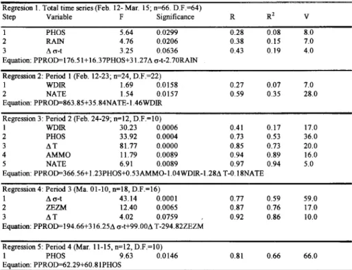
Taking into account these four main events (Fig. 3) we divided the time series in four periods, in order to discriminate the most significant covariables that explain the biomass and production variance, and at the same time, to compare which of them acted as main forcings at the respective periods. Results for regression and multiple correlations analysis are presented in Tables 3 and 4.
Phytoplankton biomass changes during the total time series (Table 3, regression I) showed that a total of 40% of the variability could be explained by four variables. The most important of them, contributing 26% of the variability was nitrite concentration, folIowed by silicate and nitrate
concentrations each contributing 5% of the
variability and rain falI contributing 4%. The results obtained by this multilinear analysis model detach the direct influence of the forcing nutrients as the most significant and, in a second leveI, the inverse influence of the rain falI (see Table m, Equation for regression 1). COJ;lsideringthe total time series, results confirm the structure for the first component derived from the PCA (Fig. 4A).
For period 1 (Table 3, regression 2), a total of 44% of the biomass variability is accounted for by rain falI. It is conc1uded that for this period interference of the second principal component occurred.
For period 2 (Table 3, regression 3), a total of 89% of explanation of the biomass variability is accounted for by four variables, the contributions of which c1early suggest the interference of the first and fourth principal components. One variable, Liat, explained 67% of the variability. One can note during this period (Feb. 24th to 29th) the evolution
and peak of total nitrogen, coinciding with
increasing variations and peaks of the stability parameters Li T and Li O' t (Figs 3H, 3D and 3E), preceded by increases of first quadrant wind speed (Figs 3A and 3B).
Table 2. Meteorological, hydrographic, chemica1and biologica1characteristics of four events during time series. Event Characteristics
1 (o Feb. 12-23)
2 (O Feb. 24-29)
Variable southwesterly and easterly winds; high rain fuIl, salinity decrease, water stability changes; total nitrogen increase; 10wphytoplankton biomass variations.
Northeasterly winds; thermal and haline stratification; total nitrogen and phyto-plankton biomass increases.
3
(V Mar. 01-10) Wind direction highly variable; progressive mixing increase; high oscilations in total nitrogen and pheopigments; significant peaks in chlorophylla.
4
(A Mar. 11-15) Strong increases in northeasterly wind speed; thermal stratification; thermocline ranging ITom5-17 m to 2-4 m; nitracline at 4m depth; euphotic zone : mixing depth
Table 3. Stepwise regression for Chlorophyll a (dependent) and significant covariables.
D.F.- degrees of fi'eedom; R- multiple corre1ation coefficient; R2_ multiple determination coefficient; V- proportion (%) of variance accounted for by each variable.
Regression 1. Total time series (Feb. 12- Mar. 15; n=66, D.F.=64)
Step Variable F Significance R
1 NITE 3.55 0.0644 0.51
2 RAIN 1.01 0.0101 0.55
3 SILI 3.58 0.0635 0.59
4 NATE 4.61 0.0359 0.61
Equation: CHL0=4.116+ 1.385NITE+0.419NATE+0.046SILI-0.141RAIN
Regression 2. Period I (Feb. 12-23; n=24, D.F.=22)
I RA\N 10.80 0.0041
Equation: CHLO=-3.118-0.I24RA\N
0.66 0.44 44.0
Regression 3. Period 2 (Feb. 24-29; n=12, D.F.=IO)
1 1\cr-t 19.25 0.0032 0.82
2 PHOS 31.80 0.0008 0.90
3 1\ T 22.51 0.0021 0.93
4 NITE 8.86 0.0034 0.95
Equation: CHL0=-4.193+1.1411\cr-t+2.2241\ T-2.675PHOS-L362NITE
0.61 0.82 0.86 0.89
61.0 15.0 4.0 3.0
Regression 4. Period 3 (Mar. 01-09; n=18, D.F.=16)
1 WDlR 4.24 0.0639
Equation: CHL0=25.384-0.061WDlR
0.11 0.50 50.0
Regression 5. Period 4 (Mar. 10-15; n=12, D.F.=IO)
I NATE 16.31 0.0009 0.80 0.64 64.0
2 ZEZM 18.96 0.0121 0.89 0.80 16.0
3 SILI 19.60 0.0115 0.95 0.90 10.0
4 NITE 16.38 0.0155 0.96 0.92 2.0
5 WDlR 4.13 0.0198 0.91 0.95 3.0
6 WSPE 1.20 0.0550 0.99 0.98 3.0
Equation: CHLO=-8.950+ 1.653NATE+ 1.551WSPE+0.194SILI+0.063WDlR-2.811NITE-2.522ZEZM
Table 4. Stepwise regression for Primary Production (dependent) and significant covariables. D.F.- degrees of fi'eedom; R- multiple correlation coefficient; R2_ multiple determinatio,n coefficient; V- proportion (%) of variance accounted for by each variable.
Regression 3: Period 2 (Feb. 24-29; n=12, D.F.=IO)
I WDlR 30.23 0.0006 0.41 0.11 11.0
2 PHOS 33.92 0.0004 0.13 0.53 36.0
3 1\ T 81.11 0.0000 0.85 0.13 20.0
4 AMMO 11.19 0.0089 0.94 0.89 16.0
5 NATE 6.91 0.0089 0.91 0.94 5.0
Equation: PPROD=366.56+ 1.23PHOS+0.53AMMO-l.04WDlR-I.2M T-0.18NATE
Regression 4: Period 3 (Ma. 01-10, n=18, D.F.=16)
I 1\cr-t 43.14 0.0001
2 ZEZM 12.40 0.0065
3 !l T 4.02 0.0159
Equation: PPROD=194.66+316.251\ cr-t+99.001\ T-294.82ZEZM
0.11 0.81 0.92
0.59 0.16 0.86
59.0 11.0 10.0
Regression 5: Period 4 (Mar. 11-15, n=12, D.F.=IO)
I PHOS 9.63 0.0146
Equation: PPROD=62.29+60.8IPHOS
0.81 0.66 66.0
R2 V
0.26 26.0 0.30 4.0 0.35 5.0 0.40 5.0
Regresion 1. Total time series (Feb. 12- Mar. 15; n=66. D.F.=64)
Step Variable F Significance R R2 V
I PHOS 5.64 0.0299 0.28 0.08 8.0
2 RAIN 4.16 0.0206 0.38 0.15 1.0
3 !l a-t 3.25 0.0636 0.43 0.19 4.0
Equation: PPROD=116.5l+ 16.31PHOS+31.211\ cr-t-2.10RAIN
Regression 2: Period I (Feb. 12-23; n=24, D.F.=22)
I WDlR 1.69 0.0158 0.21 0.01 1.0
2 NATE 1.54 0.0151 0.59 0.35 28.0
GAETA et al.: Environrnental forcing on phytoplankton and primary productivity 1-9
For period 3 (Table 3, regression 4) a total of 50% of variance is accounted for by wind direction. However it is inversely correlated with the biomass, apparently because the latter has shown a very lagged peak in relation to the wind field peak (Figs. 3A and 3J), mainly from the second quadrant. Thus, there was also intluence of the fourth component.
For period 4 (Table 3, regression 5), a total of 98% of variance is accounted for by seven variables that characterize, as in period 2, the interference of the first and fourth principal components. Nitrate concentration and euphotic zone: mixing layer ratio explained 80% of the biomass variability in this case.
When the results of the multiple regression analysis for the primary production are considered for the total time series (Table 4, regression 1), one can verifYthat 19% of variance is explained by three variables. Of those, only rain falI is common to the conjunct of variables which explains the biomass variability. Thus, primary production seemed to be intluenced by the first and fourth principal components, nevertheless with relatively low contributions.
For period 1 (Table 4, regression 2), primary production variance was directly linked to nitrate (28%) and inversely to wind direction (8%) therefore under the intluence of the first and fourth principal components.
For period 2 (Table 4, regression 3), 94% of primary production variance is accounted for by phosphate and ammonia directly (36 and 16%, :~~;-:_tively), and wind direction (17%), thermal gradient (20%) and nitrate (5%) inversely. One may conclude that for this period the first, third, and
fourth principal components determined the
phytoplankton production variability.
For period 3 (Table 4, regression 4), there was also an excelIent fitting with 86% of explanation being related to density gradient (59%), light availiability in the the I11ixing layer (17%) and thermal gradient (10%). These variab1es, as stated before, are associated to the first and fourth principal components.
FinalIy, for period 4 (Table 4, regression 5), 66% of variance is accounted for by phosphate also characterizing the interference of the first principal \.umponent.
Harmonic analysis
Harmonic analysis revealed a low frequency periodicity in the chlorophylI a (period 8.25 days)
that could be re1ated to the periodicities of the
stability parameter Li T and total nitrogen (Fig. 5), which showed two distinct significant peaks, one at a period of 6.6 days and one at a period of 4 days. Although no significant peak was observed in the wind direction and speed, data suggest a relationship, at low frequency, between atmospheric forcing and water column stratification, nitrogen availability and phytoplankton biomass changes. A second low frequency periodicity in the chlorophylIa(6.6 days)
appears to be accounted for by LiT.
The variations in the stability parameter Li ot at 1I day period also appear to be largely controlIed by the wind field. At the II day period the responses of nitrate, phosphate and silicate were in phase with the water column density structure.
.,
Discussion
Studies on horizontal diffusion using dyes led to well-defined re1ationships between the temporal and spatial scales of mixing processes (Boyce, 1974). From these re1ationships Harris (1980) defined the temporal and spatial scales that
link the time and space dimensions in the
planktonic system. Thus, for the sampling scheme of the present work, a little more than one month corresponds in horizontal and vertical spatial scale to dimensions of 1 to 50-80 km and of 0.5 to 50 m, respectively. These scales, in view of the temporal and spatial description of the phytoplankton system, are consistent with the turbulent vertical diffusion coefficient values and with the time scales of the mixing processes available in literature. The sedimenting rates are commonly in order of 0.5 m d-I (Smayda, 1970) and the dispersion of the observed sinking rates correlates well with the amplitude of variation of the vertical mixing rates calculated by Denmann & Gargett (1983).
Component I, derived from PCA, was
interpreted as the availability of new nutrients injected by continental shelf colder waters, during the pycnocline settlement, controlIed by the first quadrant winds besides. the characteristic thermal stratification processes at the summer period. The circulation patterns for the Ubatuba inner shelf region may result from interaction among the stress wind forces, rhe Coriolis force, pressure gradients and friction forces producing superficial and internal oscillations in the water column. Considering the wind fie1d (Fig. 3A and B), the required time for equilibrium among the forces is at the same order of time between the observed
oscillations from Feb. 19th and Mar. 1st,
WlND DIRECTION 20 , ... 15
10 5 O
WlND SPEED
20 , --... ... 15
10 5 O
A TEMPERA TURE
w O Z <C ã::
~
u.
O
30 20 10 O
Aa-t 40
30 .hh ____h_.._...
20 10 O 20 15 10 5 O
TOTAL NITROGEN
25 20 15 10 5 O
CHLOROPHYLL a 30
20 10 O
0.1 0.2 0.3 004 0.5 I I
I
I I I I II
11 5 3 20.1 0.2 0.3 DA 0.5 cycles.12 h-1
I I I I I I I I I
1 11 5 3 2 1 days
Fig. 5. Harmonic analysis: Periodograms.
The component n was interpreted as the transient frontal systems preceded by fourth quadrant winds (NW), and characterized by second and third quadrant winds, rain fall and turbulence periods resulting the increase of cloud covering with solar radiation reduction, addition of organic matter of continental origin to the water column and the increase of suspending matter with consequent
higher turbidity. During the sampling period at summer, apparently, the coastal waters respond permanently to preceded wind stress episodes. Since the wind does not blow constantly, OOt rather is associated to atmospheric patterns that are typical of the weather conditions, it suggests its importance both to the physical processes and to the phytoplankton system. The forcing scale at the order
PRIMARY PRODUCTlON
20=... -. -... -'''' -. ... 15
10 5 O
PHEOPIGMENTS 25
20 15 10 5 O
PHEO:CHLO 25
20 15 10 5 O
NITRATE 20
15 10 5 O
AMMONIA 20
15 10 5
o
PHOSPHATE 30
20 10 O
SIUCATE 40
GAET Aet ai..'Environrnental forcing on phytoplankton and primary productivity 21
of 200 hours strongly interacts with the
phytoplankton doubling times and the growth rates, thus affecting the competition mechanisms and the diversity of the communities (Huston, 1979).
The third component (Fig. 4B) was
interpreted as the phytoplankton responses to the turbulence and mixing processes caused by third and fourth quadrant winds which interrupt the normal first quadrant winds, typical of summer, as welI as the nutrient inputs to the system due to heavy rain fall. Phytoplankton in this region during summer have been shown to be mainly dependent on regenerated sources of nitrogen (Metzler et aI.,
1995*), and in other coastal waters, regeneration of nitrogen has been shown to supply up to 100% of the nitrogen requirements for phytoplankton (Billen, 1978; Glibert, 1982; Harrison et ai., 1983). In the
inshore Ubatuba region, the mixed layer can also receive important N03
-
and Nl4 + contributions ~y continental runoff and rain fall, mainly during summer (Braga, 1989; Susini-Zillmann, 1990). Shifts in the normal wind flow may also result in a release of nitrogen ITomthe sediment to the euphotic zone. According to Mahiques (1992), detritalorganic material ITom continental origin or ITom overlying waters deposits on the aerobic sediment and its decomposition results in an accumulation ofNl4 + aswell as NOz
-
and N03-
close to the sediment surface.Wind speed ITequency distribution showed 39% of the observations ITom O to 2.0 m S.l, 53% ITom2.0 to 6.0 m S.l and 8% ITom6.0 to 12.0 m S.l. Parallel to these values, 74% of the wind direction observations were associated to the first quadrant, 18% to the second and third quadrants and 6% to the fourth quadrant. A comparison of the time series in Figs. 3A and B shows that at most of the time the winds with intensities between 4.0 and 10.0 m S.l were ITomthe first quadrant, therefore, one can interpretate the fourth component as the forcing northeastern and eastern winds paralIel to the coast, which drive the surface coast waters transport towards the ocean and the simultaneous colder and deeper watersnormal transport towards the coast. In fact, water masses sampled, the Coast Water (CW) and the South Atlantic Central Water (SACW), confirm that their dynamics depend on the wind field, besides on the tide currents and on the bottom physiography as pointed by Castro Filho et ai.
(1987).
Observing the total inorganic nitrogen changes (Fig. 3H), one can see for period 1 (Feb. 12th
(*) Metzler, P. M.; Glibert, P. M.; Gaeta, S. A & Ludlam, 1. 1995. New and regenerated production in the South Atlantic off Brazil. In: INTERNATIONAL SYMPOSIUM ON ENVIRONMENTAL BIOGEOCHEMISTRY, BIOSPHERE AND ATMOSPHERIC CHANGES, 12. Rio de Janeiro, 1995. Abstracts. Rio de Janeiro, lseb. p. 54.
to 23th)four peaks, for period 2 (Feb. 24thto 29th)one peak, for period 3 (Mar 1stto 9th) two peaks, and for
period 4 (Mar 10thto 15th) one peak. At period 1, only the first peak (Feb. 17th)might be responding to the first quadrant winds pulse (Fig. 3A), and the second, third and fourth peaks (Feb. 18th, 19th and 23Td)might result ITom the increase of nitrogen associated to the intense rain fall observed at that time. At period 3, the second peak could be associated to turbulent mixing processes, judging the wind behavior. Thus, considering the four remaining peaks, one in each period (Feb. 17thand 28th,Mar 4th and 15th), a 200 h interval is obtained among the total nitrogen peaks. If now we compare these peaks with the values of wind direction referring to the first quadrant, the conclusion is a lag between the forcing first quadrant wind and the response of the total inorganic nitrogen in the order of 60 hours (Table 5). In the harmonic analysis (Fig. 5), it is seen that the total nitrogen peak at a 6.6 days period matches the largest peak of A T; on the other hand, a second peak at a 4 days period matches the largest peak of ammonia. It is also noticeable ITomTable 5 that the first quadrant wind leads A T by 36 hours and that A T is in phase with total nitrogen.
The phytoplankton biomass (Fig. 3J)
showed one peak at period 1 (Feb. 18th),one peak at period 2 (Feb. 28th), two peaks at period 3 (Mar. 6th and ~) and one peak at period 4 (Mar. 15th). A comparison between these peaks with those ITom the total inorganic nitrogen suggests they were in phase (Table 5). The harmonic analysis of the
phytoplankton biomass (Fig. 5) showed two
indistinguishable peaks, one at a period of 8.25 days and one at a period of 6.6 days. The former is lagged about 3 days relative to the first peak of A T and about 5 days relative to the peak of A cr t, accounting for, respectively, 17 and 26% ofvariance. The latter is in phase with the first peak of the nitrogen.
In reference to the primary production (Fig. 31), it is clear that the largest observed peak (Feb. 23Td)in all time series and the succession of oscillations between Mar. 5thand 8thwere associated with the rain falI influence and with turbulent mixing processes, while the observed peaks at Mar 3m and 15thwere likely associated exclusively with the nutrient injection by a colder and richer water mass (Fig. 3D and 3E). From Table 5 it is seen that
primary production is in phase with the
euphotic:mixed layer ratio and is lagged about two days relative to wind field forcing normal to the coast (0.302*, a positive cross correlation); about 2.5 days relative to A crtand phytoplankton biomass;
Table 5. Cross correlations: Leading factors in the first column (abbreviations as in Table I); lagged time between factors in brackets. N=64, number of lags (k) = N/4 = 16; k = 12 hours. Levels of significance: .. p<O.OI, · p<O.05.
primary production and total inorganie nitrogen (Figs 31 and 3H) suggests a lag aOOut 108 hours (Table 5).
One nonsignificant peak revealed in the harmonie analysis of primary production, accounting for 18% of variance at a period of 15 days, matehes the peaks of A <rtand ZE:ZM (Fig. 5). Phytoplankton biomass and primary production are lagged about 60 hours (Table 5). Therefore, photosynthetie eharacteristies indicate a response to the 'leading factor total nitrogen from four to five days, while the response of phytoplankton biomass is practically in phase.
In our time series in Ubatuba region, the atmospherie foreing showed a eharacteristie period of aOOut 200-264 hours and the phytoplankton biomass response ranged over the 144-192 hours time scales. The photosynthetie eharacteristics of the phytoplankton were best related to the environment 360 hours before, although their oscillations throughout the time series were lagged aOOut96-144 hours relative to nitrogen and biomass. Primary produetion responses (Fig. 31)seem to follow roughly the ZE:ZM ehanges (Fig. 3G) at a scale of days. Since tbe period between transient frontal events is approximately equivalent to the photosynthetie response time of the phytoplankton (sensu Harris,
1986), one could suppose this system as in non-steady state. At these conditions, the reserve compounds of the metaOOlicalroutes become very important and the phytoplaOkton cells can be
seen as integrators trying to buffer their internal biosynthetie pathways from external fluctuations, at
the same time they grow at rates as dose as
possible to the maximum (Morris, 1980; Eppley,
1981). With a fast uptake and storage of
nutrients, the phytoplankton may require nutrients only for brief periods during growth (McCarthy & Goldman, 1978). The populations ean continue growing rapidly as long as they are supplied with nitrogen and phosphorus at least once a week (Eppley, op. cit.). This may be the case in the
Ubatuba region as seen from Figure 5, in whieh the total nitrogen peaks at a 6.6 days period matehing the largest peak of A T, and peaks at a 4 days period matehing the largest peak of ammonia.
The 8-11 days atmospherie disturbances suggest to be major constraints regulating dynamics of the Ubatuba coastal phytoplankton assemblages. Day-to-day variations of phytoplankton standing-stock (Francos, 1996) studied at the same time series presented in this paper, showed the algal community composed by nanoflagellates and small pennate diatoms with transient appearances of dinoflagellates (Fig. 6). According to these studies, storms can play an important role in determining the phasic nature of the summer succession. At surface (Fig. 6 top) nanoflagellates peaks characterize the "after-storm" (see Fig. 3C) group of small algae, whereas at 50 and 1% light depths near 5-10% of the
standing-stock is composed by diatoms. Calm periods
GAETA et aI.:Environrnental forcing on phytoplankton and primary productivity 23
URFACE,'
i\.
!
\
.' '. ..
50% LI~.HT DEP~. . ::
...
.'
,---:
'. &_-."
.--.... o. .",.
.
_
::... :.:: :-:-:-..'-.. :'0"-. ~. """""'_' '- ./'O I I I I I 1 I I I
12 14 16 18 20 FEBRUARV
(evem1)
. .
1 3 MARCH
(event 2) (event 3) I (event 4)
Fig. 6. Day-to-day variations in the most abundant taxooomic groups of the phytoplankton at the sampling station (ftom Francos, 1996).
increasing stratification (see Fig. 3D) characterize the "pre-storm" wide dominance of nanoflagellates only at surface whereas at 50 and 1% light depths diatoms account for 25-50% of the standing-stock. Mixing caused by atmospheric disturbances has a beneficial effect on diatoms which indeed surpass nanoflagellates at surface. This re1ationship is assumed to be re1atedto the dominant hydrodynamic vertical difusive processes that enhance water nutrient concentrations (see Fig. 3H). A surface bloom composed mainly byPseudo-nitzschia sp and Dactyliosolen fragilissimus ITom 1st to 5th march
(Fig. 6 top) reinforces the relationship stated above (Francos, 1996).
In a 5-day time series conducted in the same Ubatuba region, Metzler et ai. (1995) observed an
upwelling event, during which the
N03-concentrations at the base of the euphotic zone increased over 10-fold. While primary production was observed to increase in relation to increases in N03
-,
this increase was considerably smaller,-
2-fold. No coincident increase was observed in chlorophylla.A longer time series wou1dhave been
required to determine whether such an increase eventually followed and the time scale of the lag relative to the N03
-
upwelling.It should be pointed out that our results derived ITom multivariate and harmonic analysis would not necessarily hold to other neighbouring
regions or time periods. The relevant point is that they indicate a variability in the coup1ing between both physicochemical and biological fields, which.is impelled around by, and probably at the most of time
generated by, a locally shared pattern of
environmental forcing.
Ongoing work off the Southeastern Brazil Bight, between the coastal cities of Ubatuba and Iguape, shows both in austral summer and winter a Brazil Current cyclonic meandering pattern while, at the same time, is verifying a possible correlation between this pattern and she1f break upwelling of deeper water (SACW) onto the outer continental she1f (Silva, 1994). Warm and cold-core meanders are important mechanisms for exchange of slope water across western boundary current systems, and have been shown to transport nutrients onto the continental she1f of the São Paulo State (Gaeta et aI., 1994*). In this area, during summer 1993,
nitrate concentrations in the euphotic zone over the shelf showed a gradual increasing trend in an inshore direction, ranging ITom 0.5-7.0 ~M, and upwelled nitrate (1.5-2.0 ~M) was observed in the
(*) Gaeta, S. A; BOOo,O. L. & Susini Ribeiro, S. M. M. 1994. Distributions of nitrate, chIorophylla,and primary productivity in the Southwestern Regiou of the South Atlantic During Summer. ln: SOUTHWESTERN ATLANTIC PHYSICAL OCEANOORAPHYWORKSHOP. São Paulo, 1994. AbsUacts. São Paulo, LabmonlIOUSP.p. 57~O.
2.0
.......I 1.0 J!I ãiu
.. O
o... 1.0 !li: O O
I-",
C) 0.5
z 2i z C
I-O
11) z O
1.5 I 1% LlGHT DEPTH z
C 1.0 t- .'
...I . . .'
a. O
0.5 ,o'o..:
... : :c
inner shelf and in the slope. Below the euphotic zone, nitrate values also increased gradually towards the shelf, following crudely the isobaths downstream (south) of the curving portions which diverge for several tens of kilometers. Another mechanism postulates surface variations in the mesoscale distribution of chemical and biological properties by the horizontal advection of a cold water mass originating at Cabo Frio due to a strong upwelling event (Lorenzzetti & Gaeta, 1996).
Conclusions
Our results show that wind field forcing parallel to the coast drives the stratification settlement through which SACW forcing increases nutrient availability; calm periods between storms characterize the "pre-storm" wide dominance of nanoflagellates only at surface whereas at 50 and 1% light depths, diatoms account for up to 50% of the phytoplankton standing-stock; averaged primary production values are about 0.5 gC m-2 day-I. Wind field forcing normal to the coast determines mixing which has a beneficial efIect on diatoms that dominate the water column. Rain forcing, on the other hand, leads to the "after-storm" phytoplankton assemblages at surface, characterized by small algae whereas at 50 and 1% light depths near 5-10% of the stahding-stock is composed by diatoms, and, at the same time, increases nutrient contributions by continental runofI; as a result, primary production increases over 2-fold.
Two indistinguishable significant peaks have been observed in the harmonic analysis of the phytoplankton biomass of Ubatuba coastal waters: one at a period of 8.25 days and one at a period of 6.6 days. These contribute, respectively, about 17 and 32% of the total variance of phytoplankton biomass. Total dissolved nitrogen concentrations account for most of these variations.
Two distinct significant peaks have been observed in the periodogram of the total dissolved nitrogen: one at a period of 6.6 days and one at 4 days, contributing, respectively, about 21 and 22% of the total variance. At the period of 6.6 days total nitrogen peak matches the stability parameter L\T
and at a period of 4 days matches the ammonia concentration peak.
Changes in water column stability at periods of 11-15 days suggest that it is controlled by wind field. Although wind events are known to be important sources of phytoplankton biomass changes, this study revealed that the regular periodic wind field forcing is, at least during summer, a major influence.
One non significant peak has been observed in the harmonic analysis of primary production accounting for by 18% of variance at a period of 15 days, thus being partially related to the water column stability and partially to the ratio euphotic zone:mixing depth.
In Ubatuba region, the atmospheric forcing showed a characteristic period of about 200-264 hours and the phytoplankton biomass response ranged over the 144-I92 hours time scales. The photosynthetic characteristics of the phytoplankton were best related to the environment 360 hours before, although their oscillations were lagged about 96-144 relative to nitrogen and biomass.
During summer, the interruption of steady-state conditions by transient atmospheric events and wind field intensification are the determining factors driving phytoplankton changes in this coastal environment.
Acknowledgements
The fust author acknowledges the
Fellowship Grants no. 520352/95-5 support from
the Conselho Nacional de Desenvolvimento
Científico e Tecnológico (CNPq). S. M. Susini
Ribeiro acknowledges the Post-Doctoral
Scholarship no. 97/13905-7 from Fundação de Amparo à Pesquisa do Estado de São Paulo (FAPESP); M. S. Francos acknowledges the Scholarship Grant No 91/1589-7 (FAPESP). We thank Dr. Patricia M. Glibert for valuable comments on an earlier version of the manuscript and two anonymous referees for consíTuctive criticism of the manuscript.
References
Aminot, A. & Chaussepied, M. 1983. Manuel des analyses chimiques en millieu marin. Brest, CNEXü. 395 p.
Anderson, T. W. 1971. The statistical analysis of time series. New York, John Wiley. 704p.
Billen, G. 1978. A budget of nitrogen recycling in North Sea sediments ofI the Belgian coast. Estuar. coast. mar. Sei., 7(2):127-146.
.GAETAel ai.:Environmental forcing on phytoplankton and primary productivity 25
Braga, E. S. 1989. Estudo dos nutrientes dissolvidos nas águas da Enseada das Palmas, ilha Anchieta
(Ubatuba, SP), com ênfase às formas
nitrogenadas e contribuição por aportes
terrestres e atmosféricos. Dissertação de mestrado. Universidade de São Paulo, Instituto Oceanográfico. 207p.
Castro Filho, B. M.; Miranda, L. B. de & Miyao, S.
Y. 1987. Condições hidrográficas na
plataforma continental ao largo de Ubatuba: variações sazonais e em média escala. Bolm Inst. oceanogr., S Paulo, 35(2):135-151.
Denman, K L. & Gargett, A. E. 1983. Time and space scales of vertical mixing and advection of phytoplankton in the upper oceano Limnol. Oceanogr.,28(5):801-815.
Draper, N. R & Smith, H. 1966. AppliOOregression analysis. New York, John Wiley. p. 171.
Eppley, R. W. 1981. Relations between nutrient assimilation and growth in phytoplankton with a brief review of estimates of growth rate in the oceano Cano BulI. Fish. aquat. Sci., 210:251-263.
Francos, M. S. 1996. Variações diárias sazonais (verão e inverno) do "standing-stock" do fitoplâncton e da biomassa em termos de clorofila a em duas estações fixas costeiras na
região de Ubatuba: Lat. 23°31'S - Long.
45°05'W e Lat. 23°51'S - Long. 44°56'W.
. Dissertação de mestrado. Universidade de São
Paulo, Instituto Oceanográfico. 123p.
Gaeta, S. A.; Abe, D. S.; Susini, S. M.; Lopes, R M. & Metzler, P. M. 1990. Produtividade primária, plâncton e covariáveis ambientais no Canal de São Sebastião durante o outono. Rev. Brasil. Biol.,50(4):963-974.
Glibert, P. M. 1982. Regional studies of daily, seasonal and size ftaction variability in
ammonium remineralization. Mar. Biol.
70:209-222.
Grasshoff, K; Ehrhardt, M. & Kremling, K 1983. Methods of seawater analysis. 2nd 00. New York, Verlag Chemie. 419 p.
Harris, G. P. 1980. Temporal and spatial scales in phytoplankton ecology. mechanisms, methods, models, and management. Cano J. Fish. aquat. Sci.,37(5):877-900.
Harris, G. P. 1986. Phytoplankton ecology: structure, function and fluctuation. 1st 00. New York,
Chapman and HalI. 384 p.
Harrison, W. G.; Douglas, D.; Falkowski, P.; Rowe, G. & Vidal, J. 1983. Summer nutrient dynamics of the Middle Atlantic Bight: nitrogen uptake and regeneration. J. Plankt. Res. 5(4):539-556.
Huston, M. 1979. A general hypothesis of species diversity. Am. Nat., 113(1):81-101.
JefITey, A. D. & Humphrey, G. F. 1975. New spectrophotometric equations for determining chlorophylIs a, b, c1 and c2 in higher plants, algae, and natural phytoplankton. Biochem. Physiol. Ptl., 167:191-194.
Jenkins, G. M. & Watts, L. G. 1968. Spectral analysis and its applications. San Francisco, Holden-Day. 525p.
Kutner, M. B. B. 1961. Algumas diatomáceas encontradas sobre algas superiores. Bolm Inst. oceanogr., S Paulo, 11(3):3-11.
Kutner, M. B. B. & Sassi, R 1979. DinoflagelIates ftom the Ubatuba region (Lat. 230)0'S-Long. 45°06'W) Brazil. In: Taylor, D. L. & Seliger, H. OOsToxic dinoflagelIates blooms. New York, Elsevier.p.169-172.
Legendre, L. & Legendre, P. 1984a. Écologie numérique. 1. Le traitement multiple des données écologiques. 2c éd. Québec, Masson Presses de l'Université du Québec. 26Op.
Legendre, L. & Legendre, P. 1984b. Écologie
numérique. 2. La structure des données
écologiques. 2c éd. Québec, Masson Presses de l'Université du Québec.335p.
Lorenzen, C. J. & JefITey,S. W. 1980. Determination of chlorophylI in seawater. UNESCO tech. Papo mar. Sei., 35:1-20.
Lorenzzetti, J. A. & Gaeta, S. A. 1996. The Cape Frio Upwelling effect over the South Brazil Bight northern sector shelf waters: a study using
AVHRR images. Int. Arch. Photogramm.,
31(7):448-453.
Margalef, R 1978. Life-forms of phytoplankton as
survival alternatives in an unstable
enviromnent. Oceanol. Acta, 1(4):493-509.
McCarthy, J. J. & Goldman, J. C. 1979. Nitrogenous nutrition of marine phytoplankton in nutrient-depletOOwaters. Science,203:670-672.
Millard, R c.; Owens, W. B. & Fofonotf, N. P. 1990. On the calcu1ation of the Brunt-Vãisã1a frequency. Deep-Sea Res., 37(lA):167-181.
Morris, I. 1980. Paths of carbon assimilation in marine phytoplankton. In: Falkowski, P. 00. Primary productivity in the sea. New York, P1enumPress. p. 139-160.
Oliveira, I. R 1980. Distribuiçãodas diatomáceas.
epifiticas na região de Ubatuba. Dissertação de mestrado. Universidade de São Paulo, Instituto Oceanográfico. 88p.
Perazza, M. C. D. 1982. Variação sazonal do fitoplâncton e fatores ambientais na Enseada do°
F1amengo (Lat. 23DJO'S-Long. 45 06'W):
algumas considerações metodológicas.
Dissertação de mestrado. Universidade de São Paulo, Instituto Oceanográfico. 105p.
P1att, T. & Denman, K. L. 1975. Spectral ana1ysisin ecology. A. Rev. Ecol. Syst., 6:189-210.
Sassi, R 1978. Variação sazonal do fitoplâncton e fatores ecológicos básicos da região do Saco da Ribeira (Lat. 23°30'S-Long. 45°07'W), Ubatuba, Brasil. Dissertação de mestrado. Universidade de São Paulo, Instituto Oceanográfico. 147p.
Sassi, R & Kutner, M. B. B. 1982. Variação sazonal do fitoplâncton da região do Saco da Ribeira (Lat. 23DJO'S;Long. 45°07'W). Ubatuba,
Brasil. Bolm Inst. oceanogr., S Paulo,
31(2):29-42.
Silva, M. P. 1994. Caracterização fisico-química das massas de água da Bacia de Santos durante o Projeto COROAS. Verão e inverno de 1993. Dissertação de mestrado. Universidade de São Paulo, Instituto Oceanográfico. 135p.
Smayda, T. J. 1970. The suspension and sinking of phytoplankton in the sea. Oceanogr. mar. Bio. a. Rev.,8:353-414.
Soares, F. S. 1983. Estudo do fitoplâncton de águas costeiras e oceânicas da região de Cabo Frio-RJ (23°31'S-41°52'W) até o Cabo de Santa Marta Grande-SC (28°43'S-47°57'W). Dissertação de mestrado. Universidade de São Paulo, Instituto Oceanográfico. 118p.
Susini-Zillmann, S. M. 1990. Distribuição sazonal do fitoplâncton na radial entre ilha Anchieta e ilha da Vitória (Lat. 23DJ1'S-Long. 45°06'W à Lat. 23°45'S-Long. 45°01'W) da região de Ubatuba, São Paulo. Dissertação de mestrado.
Universidade de São Paulo, Instituto
Oceanográfico.2v.
Teixeira, C. 1973. Preliminary studies of primary production in the Ubatuba region (Lat. 23DJO'S-Long. 45°06'W), Brazil. Bolm Inst. oceanogr., S Paulo, 22:49-58.
Teixeira, C. 1979. Produção primária e algumas considerações ecológicas da região de Ubatuba (Lat. 23°30'S-Long. 45°06'W), Brasil. Bolm Inst. oceanogr., S Paulo, 28(2):23-28.
Teixeira, C. 1980. Estudo quantitativo da produção primária, clorofila a e parâmetros abióticos em
relação à variação temporal (Lat. 23DJO'S-Long. 45°06'W). Tese de livre-docência. Universidade de São Paulo, Instituto Oceanográfico. 243p.
Teixeira, C. & Tundisi, J. G. 1981. The etfects of
nitrogen and phosphorus enrichments on
phytoplankton in the region of Ubatuba (Lat. 23°30'S-Long. 45°06'W), Brazil. Bolm Inst. oceanogr., S Paulo, 30(1):77-86.
Teixeira, C. 1986. Daily variation ofmarine primary production in the Flamengo Inlet, Ubatuba region, southern Brazil. In: Bicudo, C. E. M.; Teixeira, C. & Tundisi, J. G. eds Algas: a energia do amanhã. Universidade de São Paulo, Instituto Oceanográfico. p. 97-108.
Teixeira, C. & Gaeta, S. A. 1990. Contribution of picoplankton to primary production in estuarine, coastal and equatorial waters of Brazil. Hydrobiologia, 209(2): 117-122.
GAETA et aI.: Environrnental forcing on phytoplankton and primary productivity 27
Turpin, D. H. & Harrison, P. 1. 1979. Limiting nutrient patehiness and its role in phytoplankton ecology. J. exp. mar. Biol. Eeol., 39:151-166.
UNESCO 1981a. Baekground papers and supporting data on the Practical Salinity Seale. 1978. UNESCOtech. Papomar. Sei., 37:1-144.
UNESCO 1981b. Baekground papers and supporting data on the lnternational Equation of State of Seawater 1980. UNESCO teeh. Papo mar. Sei., 38:1-192.