GARMA models, a new perspective using Bayesian methods and transformations

(1)

GARMA models, a new perspective using

Bayesian methods and transformations

(2)

(3)

UNIVERSIDADE FEDERAL DE SÃO CARLOS CENTRO DE CIÊNCIAS EXATAS E TECNOLOGIA

PROGRAMA INTERINSTITUCIONAL DE PÓS-GRADUAÇÃO EM ESTATÍSTICA UFSCar-USP

Breno Silveira de Andrade

GARMA models, a new perspective using Bayesian methods and

transformations

Doctoral dissertation submitted to the Departa-mento de Estatística - DEs - UFSCar and to the Instituto de Ciências Matemáticas e de Computação - ICMC-USP, in partial fulfillment of the requirements for the degree of the Doctorate Joint Graduate Pro-gram in Statistics DEs-UFSCar/ICMC-USP. FINAL VERSION

Advisor: Prof. Dr. Marinho Gomes de Andrade Filho

(4)

(5)

UNIVERSIDADE FEDERAL DE SÃO CARLOS CENTRO DE CIÊNCIAS EXATAS E TECNOLOGIA

PROGRAMA INTERINSTITUCIONAL DE PÓS-GRADUAÇÃO EM ESTATÍSTICA UFSCar-USP

Breno Silveira de Andrade

Modelos GARMA, uma nova perspectiva usando métodos

Bayesianos e transformações.

Tese apresentada ao Departamento de Estatística -Des/UFSCar e ao Instituto de Ciências Matemáticas e de Computação - ICMC-USP, como parte dos requisitos para obtenção do título de Mestre ou Doutor em Estatística - Programa Interinstitucional de Pós-Graduação em Estatística UFSCar-USP. VERSÃO FINAL

Orientador: Prof. Dr. Marinho Gomes de Andrade Filho

(6)

(7)

Agradecimentos

Agradeço, primeiramente a Deus e Nossa Senhora. Agradeço também:

A meus pais e demais familiares.

A Paula, pelo amor, amizade e total apoio.

A todos os amigos que sempre estiveram presentes, contribuindo com discussões, críticas e sugestões.

Ao professor Marinho Gomes de Andrade Filho, pela orientação segura, e pelo incentivo durante todo o curso de pós-graduação. Ao professor Jacek Le´skow, pela orientação durante meu doutorado sanduíche.

(8)

(9)

Abstract

Generalized autoregressive moving average (GARMA) models are a class of models that was developed for extending the univariate Gaussian ARMA time series model to a flexible observation-driven model for non-Gaussian time series data. This work presents the GARMA model with discrete distributions and application of resampling techniques to this class of models. We also proposed The Bayesian approach on GARMA models. The TGARMA (Transformed Generalized Autoregressive Moving Average) models was proposed, using the Box-Cox power transformation. Last but not least we proposed the Bayesian approach for the TGARMA (Transformed Generalized Autoregressive Moving Average).

Keywords: Transformed Generalized ARMA model, Generalized

(10)

(11)

Resumo

Modelos Autoregressivos e de médias móveis generalizados (GARMA) são uma classe de modelos que foi desenvolvida para extender os conhecidos modelos ARMA com distribuição Gaussiana para um cenário de series temporais não Gaussianas. Este trabalho apresenta os modelos GARMA aplicados a distribuições discretas, e alguns métodos de reamostragem aplicados neste contexto. É proposto neste trabalho uma abordagem Bayesiana para os modelos GARMA. O trabalho da continuidade apresentando os modelos GARMA transformados, utilizando a transformação de Box-Cox. E por último porém não menos importante uma abordagem Bayesiana para os modelos GARMA transformados.

Palavras-chave: ARMA Transformado Generalizado, ARMA

(12)

(13)

List of Figures

2.1 Estimated densities with Monte Carlo and bootstrap negative binomial 14

2.2 Estimated densities with Monte Carlo and bootstrap binomial . . . . 15

2.3 Estimated densities with Monte Carlo and bootstrap Poisson . . . . 15

2.4 Graph of Number of Hospitalizations caused by dengue . . . 17

2.5 ACF and PACF for number of hospitalizations caused by dengue . . 17

2.6 Graph of bootstrap densities of each parameter . . . 19

2.7 Adjusted values versus real values of Number of Hospitalizations caused by dengue . . . 19

2.8 Residual Analysis of Hospitalizations caused by dengue . . . 20

2.9 Predictions with GARMA(1,0) Negative Binomial model with Hospitalizations caused by dengue series . . . 20

2.10 Graph of Morbidity in São Paulo . . . 21

2.11 ACF and PACF for Morbidity in São Paulo . . . 21

2.12 Graph of bootstrap densities of each parameter . . . 23

2.13 Adjusted values versus real values of Monthly Morbidity in São Paulo 23 2.14 Residual Analysis of Monthly Morbidity in São Paulo . . . 24

2.15 Predictions with GARMA(2,0) negative binomial model with Monthly Morbidity in São Paulo . . . 24

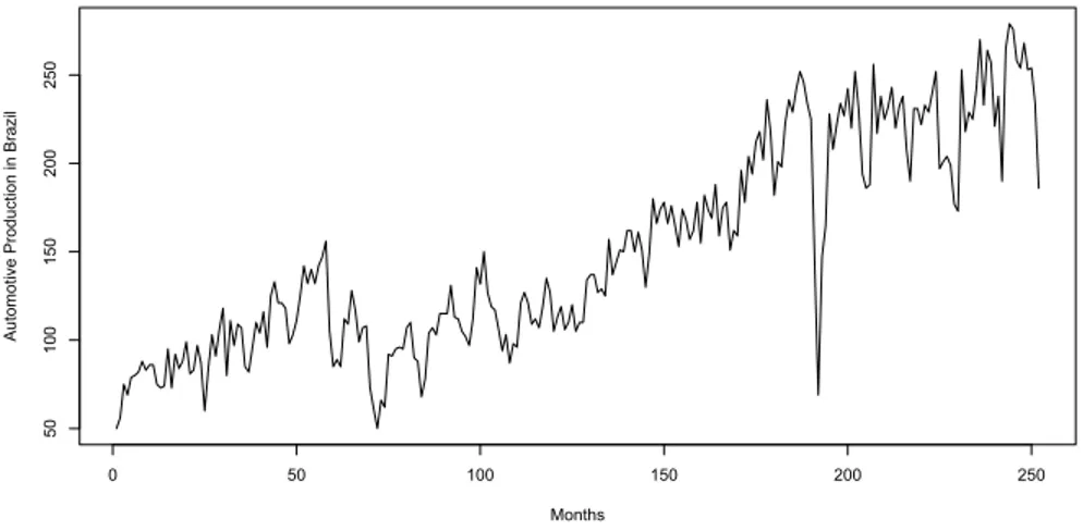
3.1 Graph of number of automobile production in Brazil. . . 35

(18)

3.4 Number of hospitalizations caused by Dengue Fever. . . 38

3.5 Residual Analysis of Hospitalizations caused by Dengue. . . 39

3.6 Predictions with GARMA(1,2) Negative Binomial model with Hospitalizations caused by Dengue series. . . 40

3.7 Number of deaths in Brazil. . . 40

3.8 Residual analysis of the number of deaths in Brazil. . . 41

3.9 Predictions with GARMA(1,0) Binomial model with Number of death in Brazil series. . . 42

4.1 Densities of parameters with λ= 0.3 . . . 51

4.2 Densities of parameters with λ= 0.5 . . . 52

4.3 Bootstrap densities for TGARMA models . . . 54

4.4 Graph of Annual Swedish fertility rates . . . 56

4.5 Auto Correlation Function and Partial Auto Correlation Function of Annual Swedish fertility rates . . . 56

4.6 λempirical bootstraped density Annual Swedish fertility rates . . . . 57

4.7 Graph of true values versus the estimated values of the residuals of Annual Swedish fertility rates series . . . 58

4.8 Autocorrelation function and partial autocorrelation function of the residuals of rate of Annual Swedish fertility rates series . . . 59

4.9 Original Predictions with GARMA(1,0) Gamma model with Rate of Annual Swedish fertility rates series . . . 59

5.1 Graph of Annual Swedish fertility rates . . . 73

5.2 Auto Correlation Function and Partial Auto Correlation Function of Annual Swedish fertility rates . . . 73

5.3 Autocorrelation function and partial autocorrelation function of the residuals of rate of Annual Swedish fertility rates series . . . 75

(19)

List of Tables

2.1 Negative Binomial GARMA(1,1) Confidence intervals n=100 . . . 14

2.2 Binomial GARMA(1,1) Confidence intervals n=100 . . . 15

2.3 Poisson GARMA(1,1) Confidence intervals n=100 . . . 16

2.4 Model Selection Criteria using Number of Hospitalizations caused by dengue . . . 18

2.5 Estimates of Hospitalizations caused by dengue series with GARMA(1,0) Negative Binomial. . . 18

2.6 Model Selection Criteria using Monthly Morbidity in São Paulo . . . 22

2.7 Estimates of Monthly Morbidity in São Paulo series with GARMA(2,0) negative binomial . . . 22

3.1 Parameters values to simulate from Negative Binomial GARMA(p,q). 32

3.2 Monte Carlo experiments. Corrected bias, corrected errors and mean acceptance rates for the Bayesian estimation of Negative Binomial GARMA(p,q) model. . . 34

3.3 Proportions of correct model chosen via Bayesian criteria with Negative Binomial GARMA(p,q) models. . . 34

3.4 Bayesian selection criteria for the number of automobile production in Brazil. . . 36

3.5 Estimation results. GARMA(1,1) Negative Binomial model for number of automobile production in Brazil.. . . 36

(20)

3.8 Bayesian selection criteria using the number of deaths in Brazil.. . . 41

3.9 Estimates of the number of deaths in Brazil series with GARMA(1,0) Binomial. . . 41

4.1 Gamma GARMA(p,q) real values . . . 50

4.2 TGARMA(1,1) with gamma distribution and Box-Cox power transformation . . . 51

4.3 Proportions of correct model using BIC with gamma TGARMA(p,q) model . . . 52

4.4 TGARMA(2,2) with Gamma distribution and Box-Cox Power transformation . . . 53

4.5 Bootstrap TGARMA(1,1) Gamma . . . 54

4.6 Coverage Bootstrap TGARMA(1,1) Gamma . . . 55

4.7 Criterion selection using Annual Swedish fertility rates . . . 57

4.8 Estimates of Annual Swedish fertility rates series with TGARMA(1,0) Gamma . . . 58

5.2 Proportions of correct model chosen using Bayesian criterion with Gamma GARMA(p,q) model. . . 71

5.4 Criterion selection using Annual Swedish fertility rates . . . 74

(21)

C

HAPTER

1 Introduction

Counts as observations have attracted significant attention from time series specialists recently. Different contexts present such kind of data: the number of incidences of a certain disease (Poliomyelitis in U.S. Zeger (1988) and Asthma cases in a hospital in Campbelltown, Davis et al. (1999)). Integer financial data sets, like the number of transaction price movements were also discussed (see for example,Liesenfeld et al. (2006) andRydberg and Shephard (2003)). There are important data sets coming from Brazil like the number of automobile production in Brazil, the number of hospitalizations caused by Dengue Fever and number of death in Brazil that will be analyzed.

Parameter and observation driven models provide a flexible framework for modelling time series of counts. So far, a wide variety of models for count time series have been discussed in literature usually embedded in the framework of integer valued ARMA type models (see for exampleBiswas and Song(2009)). An overview of these kind of models can be found inDavis et al. (1999) while Zeger

(1988) and Chan and Ledolter (1995) explicitly discuss and develop estimation techniques for Poisson generalized linear models with an autoregressive latent process in the mean.

(22)

counts which can account for discreetness, overdispersion and serial correlation.

Zhu(2010) proposed a negative binomial INGARCH model applied to polio data. Modelling polio data was also discussed inZeger(1988).

The focus of this research are GARMA models, Bayesian methods, transformations and applications. The motivation for our work comes from the observation-driven model developed by Benjamin et al. (2003). The real advantage of GARMA models is in providing an exact parametrization of conditional distributions with the help of exponential family. Therefore, in GARMA models, the likelihood can be explicitly expressed for any fixed set of parameter values. Such models can also be used with a variety of time-dependent response variables.

Important aspect of the Chapter2 is the application of resampling techniques to GARMA models. One of the advantages of the resampling procedures is to improve the evaluation of the confidence intervals and coverage probabilities. Resampling methods in time series context have significant advantage over the classical methods based on asymptotic distributions. In resampling approach confidence intervals are created directly from the sampling distributions of the estimators. The role of resampling is to approximate such sampling distributions. GARMA models are no exception to this rule and we provide both theoretical and real data evidence for that.

The idea of resampling is based on approximating the sampling distribution of an estimator _θˆ _{via an empirical counterpart based on replicates. In the}

case of dependent data, one has to carefully introduce resampling techniques while approximating a sampling distribution of _θˆ_{. For a more elaborate study of}

resampling techniques for nonstationary time series the reader is refereed e.g. to

Le`skow and Synowiecki(2010).

There is an extensive research dedicated to resampling for independent data structures. Efron (1979) introduced the method and presented fundamental results using resampling techniques. Resampling methods for times series have been discussed in the mongraph of in Lahiri (2003). In this context one has to mention pioneering work of Bühlmann (2002), Politis (2003) and Härdle et al.

(23)

has been developed by Le`skow and Synowiecki (2010), Dehay et al. (2014) and

Dudek et al.(2014a).

The Chapter 3 extends the work of Benjamin et al. (2003), giving rise to the Bayesian approach on the generalized autoregressive moving average (GARMA) model. This approach presents some gain in terms of estimation, that could be more adequate using different loss functions. The use of Bayesian selection criteria is also an import contribution from this article. Last but not least the application of discrete models on important Brazilian real data providing a new perspective on this field.

In the Chapter4we propose using Box-Cox transformations in order to be able to describe our data with GARMA model. Therefore, de Andrade et al. (2016b) proposed model is TGARMA (Transformed Generalized Autoregressive Moving Average). The use of transformations have been shown a good alternative to reduce these kind of problems. Hamasaki and Kim (2007) described a Box and Cox power-transformation to confined and censored nonnormal responses in regression. da Silva et al. (2011) proposed the use of Box-Cox transformation and regression models to deal with fecal egg count data.Gillard(2012) presented a study using Box-Cox family of transformations, the paper comments about problems with asymmetry in the transformed data. Castillo and F.G. (2013) commented about many fields where the Box-Cox transformation can be used, and also proposed a method to improve the forecasting models. Ahmad et al.

(2015) combined Box-Cox and bootstrapping idea in one algorithm, the Box-Cox is to ensure the data is normally distributed and bootstrap to deal with small and limited sample size data.

The transformation parameter λ is estimated using the profile likelihood (PL).

Moreover, we assess the correctness of the choice ofλ using bootstrap method.

This method provides confidence intervals forλ. The partial likelihood method was

introduced byCox (1975) and is based entirely on the conditional distribution of the current response, given past responses, and past covariates information and functions thereof can be used for inference. Zhu and Ghodsi (2006) presented a procedure to dimensionality selection maximizing a profile likelihood function.

(24)

our main contribution concerns inference under the Bayesian framework providing MCMC procedures to evaluate the joint posterior distribution of model parameters.

de Andrade et al. (2016a) presented a Bayesian approach for GARMA models, indicating advantages of using the Bayesian methods.

The Chapter 5 extends the TGARMA models, giving rise to the Bayesian approach on the transformed generalized autoregressive moving average (TGARMA) model. This approach presents some gain on the estimate, that could be more adequate using different loss functions. A prior distribution on the parameter λ add information of this parameter, also the posterior density

guarantee properties on the transformation parameter. The using of Bayesian selection criterion is also an import gain on this article. Properties of MCMC were used to improve the predictions and construct confidence intervals. Last but certainly not least the application of Swedish fertility rates.

The remainder of this work is organized as follows. Chapter 2 defines the GARMA model with discrete distributions and application of resampling techniques to this class of models. The Bayesian approach on GARMA models are presented in Chapter 3. The Chapter 4 the TGARMA (Transformed Generalized Autoregressive Moving Average) is proposed. The Chapter 5

(25)

C

HAPTER

2 GARMA models and moving block

bootstrap

Abstract

Generalized autoregressive moving average (GARMA) models were devel-oped to extend the univariate Gaussian ARMA time series. In particular, such models can be applied to describe discrete time series. Our paper discusses the Moving Block Bootstrap (MBB) to improve the inference for the parameters of the GARMA model. We provide consistency theorem for MBB applied to GARMA models. Real data related to morbidity caused by external causes considering children younger than 1 year in São Paulo and hospitalizations caused by dengue disease in Ribeirão Preto state of São Paulo in Brazil are analyzed using our approach.

2.1 Generalized Autoregressive Moving Average (GARMA)

model

2.1.1 Model Definition

(26)

information setFt−1 = (y1, . . . , yt−1, µ1, . . . , µt−1). The conditional density belongs

to exponential family and is given by

f(yt|Ft−1) = exp

ytαt−b(αt)

ϕ +d(yt, ϕ)

, (2.1)

whereαt and ϕ are canonical and scale parameters, respectively. Moreover b(·) and d(_·) are specific functions that define the particular exponential family. The

conditional mean and conditional variance ofytgivenFt−1 are represented as:

µt=b′(αt) = E(yt|Ft−1) (2.2)

V ar(yt|Ft−1) = ϕb′′(αt), witht = 1, . . . , nandy1,. . .,ynare observed.

Following the Generalized Linear Models (GLM) approach the parameterµt is related to the predictorηtby a twice differentiable one-to-one monotonic function

g, called link f unction. In general, we can also include the set of covariates

x into our model. Moreover, we can we add an additional component allowing

autoregressive moving average terms to be included. In such a case our model will have a form:

g(µt) = ηt =x′tβ+ p X

j=1

φj{g(yt−j)−x′t−jβ}+ q X

j=1

θj{g(yt−j)−ηt−j}. (2.3)

The parametersp and q are identified using the classical BIC or AIC criteria.

For more information the reader is refereed toKedem and Fokianos(2002) andLi

(1994).

The GARMA(p,q) model is defined by the equations (2.1) and (2.3). For certain functions g, it may be necessary to replace yt with ynew in (2.3) to avoid the non-existence of g(yt) for certain values of yt. The form ynew depends on the particular functiong and is defined for specific cases later.

(27)

2.1 Generalized Autoregressive Moving Average (GARMA) model

are important to relate the interest exponential family distribution to the predictor.

2.1.2 Poisson GARMA model

Suppose thatyt|Ft−1 follow Poisson distribution with meanµt, thus

f(yt|Ft−1) = exp{ytlog(µt)−µt−log(yt!)}. (2.4) Here, Yt|Ft−1 has a distribution in the exponential family with ϕ = 1 , αt =

log(µt),b(αt) = exp(αt),c(yt, ϕ) =−log(yt!)andν(µt) = µt.

The canonical link function for this model is the logarithmic function, thus the linear predictor is given by

log(µt) = β0+

p X

j=1

φj{logynewt−j}+ q X

j=1

θj{log(ytnew−j)−log(µt−j)}. (2.5)

In the equation aboveynew

t−j = max(yt−j, c),0< c <1. In sequel we will drop the superscript′′_new′′ _{understanding that we truncate}_y

tfrom below we needed. The Poisson GARMA model is defined by the equations (2.4) and (2.5).

2.1.3 Binomial GARMA model

Suppose thatyt|Ft−1 follows a binomial distribution with the meanµt, thus

f(yt|Ft₋1) = exp

ytlog

µt

m−µt

+mlog

m₋µt

m

+ log

Γ(m+ 1)

Γ(yt+ 1)Γ(m−yt+ 1)

. (2.6)

The canonical link function for this model is the logarithmic function. The linear predictor is given by

log

µt

m₋µt

=β0+

p X

j=1

φj{logyt−j}+ q X

j=1

θj{log(yt−j)−log(µt−j)}, (2.7)

(28)

2.1.4 Negative Binomial

Letyt a time series such that,yt|Ft−1 ∼N B(k, µt), thus

f(yt|Ft−1) = exp

ytlog

µt

µt+k

+klog

k µt+k

+ log

Γ(k+yt)

Γ(yt+ 1)Γ(k)

,

(2.8) that belongs to exponential family withk known

The link function for this model is the logarithmic function

log

µt

µt+k

=β0+

p X

j=1

φj{logyt−j}+ q X

j=1

θj{log(yt−j)−log(µt−j)}, (2.9)

2.1.5 Seasonal Component

The seasonal components of the model will be represented as βS1 and βS2,

using functionscos and sinrespectively. These two terms will be included in the

predictor, thus

log(µt) = β0+βS1cos

2πt

12

+βS2sin

2πt 12 + + p X j=1

φj{logyt−j}+ q X

j=1

θj{log(yt−j)−log(µt−j)}. (2.10)

The next subsection contains the Maximum Likelihood Estimation MLE for the GARMA models.

2.1.6 Maximum Likelihood Estimation and Inference

(29)

Let _{yt} be a time series where the equations (2.1) and (2.3) are satisfied. The parameter vector is γ′ _{= (}_β′_{, φ}′_{, θ}′₎_{, where} _β _{= (}_β

0. . . βm)′, φ = (φ1. . . φp)′ and alsoθ = (θ1. . . θq)′. For the estimation procedure the approximated likelihood function in the r first observations is used. Fr = {y1. . . yr}, where r = max(p, q). The partial likelihood function can be constructed considering thatyt−1 andytare conditionally independent. Thus

L(β, φ, θ_|Fn) ∝ n Y

t=r+1

f(yt|Ft)

∝

n Y

t=r+1

exp

ytg(µt)−b(g−1(µt))

ϕ +c(yt, ϕ)

, (2.11)

whereg(µt)is the link function given by

g(µt) = x′tβ+ p X

j=1

φj{g(yt−j)−x′t−j}+ q X

j=1

θj{g(yt−j)−g(µt−j)}. (2.12)

In the above equationst=r+ 1, . . . , n. The equations (2.11) and (2.12) do not

have a closed form solution therefore a numerical optimization routine will be used.

The GARMA models present interesting asymptotic characteristics, see

Benjamin et al.(2003). This theory works well to big data sets, however in discrete real data is common deal with small data sets. The resampling methods can be a solution to asymptotic problems.

2.1.7 Predictions with GARMA models

Prediction plays a key role in time series analysis. The estimate ηˆt, for t =

r+ 1, . . . , nare obtained by

ˆ

ηt=xtβˆ+ p X

j=1

ˆ

φj{g(yt−j)−xt−jβˆ}+ q X

j=1

ˆ

θj{g(yt−j)−ηˆt−j} (2.13)

Using this equation (2.13), the mean of the process is given by µˆt = g−1(ˆηt), fort=r+ 1, . . . , n.

(30)

where the information untilnwere known. And also

Fn+1 ={xn+1, xn, . . . , x1, yn, yn−1, . . . , y1, µn, µn−1, . . . , µ1}.

ˆ

yt+h is called prediction with originnand horizonh. The prediction for GARMA models is made recursively by the linear predictor of each model. Using the MLE estimate can be obtained

ˆ

ηn+1 =xn+1βˆ+

p X

j=1

ˆ

φj{g(ˆyn−j+1)−xn−j+1βˆ}+

q X

j=1

ˆ

θj{g(ˆyn−j+1)−ηˆn−j+1}. (2.14)

Thus the prediction 1 step ahead(h = 1) is calculated by yˆn+1 = g−1(ˆηn+1) =

µn+1, where

ˆ

yt−j+h =yt−j+h, h≤j

ˆ

yt−j+h =g−1(ˆηt−j+h), h > j Forh >1

ˆ

ηn+h =xn+hβˆ+ p X

j=1

ˆ

φj{g(ˆyn−j+h)−xn−j+hβˆ}+ q X

j=1

ˆ

θj{g(ˆyn−j+h)−ηˆn−j+h}, (2.15)

Confidence intervals for predictions present the idea of more information about the forecast values. In GARMA models, the predictive distribution does not follow a Gaussian density, thus, the usual method based on the asymptotic confidence intervals, evaluated with the unconditional variance, are not the most appropriate. Therefore, the confidence intervals for predictions will be evaluated using quantiles of the estimated distribution. The Algorithm used to calculate the CI(1−δ) for

predictions is the follow:

Confidence Interval Algorithm

STEP 1 Let a sequence of forecast values _byt+h forh= 1, . . . , H.

STEP 2 Take h= 1,k = 0,y_t(0)₊_h = 0,S_t(0)₊_h = 0 and also initiateLB = 0,U B=0.

(31)

f(y(_t₊k)_h_|β(j),Φ(j),Θ(j),Fbt+h) = exp

y_t(₊k)_hα_t(₊j)_h₋b(α_t(j₊)_h)

ϕ +d(y

(k)

t+h, ϕ) !

,

(2.16) and also,

b

p(y_t(₊k)_h_|Fbt+h) =

1

Q

Q X

j=1

f(y(_t₊k)_h_|β(j),Φ(j),Θ(j),Fbt+h). (2.17)

STEP 4 Usingp_b(y_t(₊k)_h_|Fbt+h)computeSt(+k+1)h with

S_t(₊k+1)_h =S_t(₊k)_h+p_b(y_t(₊k)_h_|Fbt+h) (2.18)

STEP 5 IfLB = 0andS_t(₊k+1)_h _≥δ,_→yt+h,δ =y(_t₊k)_h andLB = 1.

STEP 6 IfU B = 0 andS_t(₊k+1)_h _≤(1₋δ),_→yt+h,(1−δ) =yt(+k)h andU B = 1.

STEP 7 If LB = 0 or U B = 0, take k = k+ 1 and y_t(₊k)_h = y_t(₊k−_h1) + 1, repeat steps 3

and 4 untilLB = 1 andU B = 1.

The percentiles100δ%and100(1₋δ)%are represented byyt+h,δ andyt+h,(1−δ)

respectively, and given by:

yt+h,δ = max (

y_t(₊r)_h

r X

k=1

b

p(y(_t₊k)_hbFt+h)≤δ )

. (2.19)

yt+h,(1−δ)= min

(

y_t(₊r)_h

r X

k=1

b

p(y_t(₊k)_hbFt+h)≥(1−δ) )

. (2.20)

The confidence interval100(1₋δ)%for the predictions is given by:

CI(1−δ) =yt+h,δ;yt+h,(1−δ)

(32)

confidence intervals in the time series field. The next section introduces the concept of bootstrap applied in GARMA models.

2.2 Resampling methods

Resampling methods are based on recalculating the value of the estimator on samples that are drawn from the initial sample in a special way. In such a way we obtain an approximation of the distribution of the investigated estimator. This technique in the time series context is computationally intense as one has to many times recalculate complicated algorithms. Therefore, fast computing is a key.

Since Efron (1979) seminal paper, bootstrap algorithms have generated considerable attention. Two main characteristics explain their popularity. Due to bootstrap approach we are able to approximate the sampling distribution of an estimator more effectively than using asymptotic counterparts. This is especially true in time series context, where frequently the asymptotic distribution may have parameters that are not estimable in practice. Resampling methods also allow computing valid asymptotic quantiles of the limiting distribution in different situations, even when the limiting distribution is unknown. One has to bear in mind, however, that before using a given resampling routine we have to prove its consistency. Consistency of resampling means that for increasing sample size the quantiles produced by resampling converge to quantiles of the corresponding asymptotic distribution.

2.2.1 Moving Block Bootstrap

The MBB algorithm was intensively studied, the algorithm and many examples can be found in the mongraph ofLahiri (2003). We will present the assumptions to guarantee the consistency of the MBB applied on the GARMA models.

Theorem 4.1Let the following assumptions be fulfilled:

A1 _{yt} time series that follows GARMA model (2.1) and (2.3) with parameters

γ = (β, φ, θ)

A2 _{yt} fulfills the α-mixing condition with P∞τ=1α(τ) < ∞. Moreover the

following moment continuity condition is fulfilled

(2 + δ moment condition): There exist δ > 0,r _∈ [0,1 +δ)and nonnegative

(33)

2.2 Resampling methods

Eh_|Yt−µt|2+δ µt

i

≤d1|µt|r+d2

Under assumptions (A1)and (A2)the MBB resampling method is consistent.

This means that

sup

x |

P r∗_{√n( ˆγ∗

n−γˆn)≤x} −P r{√n( ˆγn−γn)≤x| P

−→0 (2.21)

In the formula above the inequalities are understood coordinatewise.

Remark: Due to the assumptions of GARMA models we have the existence of

all moments. Therefore, the requirement on the rate of convergence of mixing function is weaker than in a general stationary case. The conditional second moment continuity condition is fulfilled e.g. for Poisson GARMA models and binomial GARMA models with fixed m. For general discussion of consistency of conditions for time series the reader is refereed to Dudek et al. (2014b) or to mongraph ofLahiri(2003).

Proof of the Theorem: We start our proof by noting that any time series _{yt} fulfilling the conditions(A1) and (A2) of GARMA model is stationary in the strict

sense. See Woodard et al. (2011) Theorem 14, page 815. Strict stationary of

{yt} together with mixing condition P∞_τ₌₁α(τ) < ∞ provides for consistency of MBQRB procedure: seeLahiri (2003) and also Dudek et al. (2014b) for detailed arguments.

2.3 Simulation Study

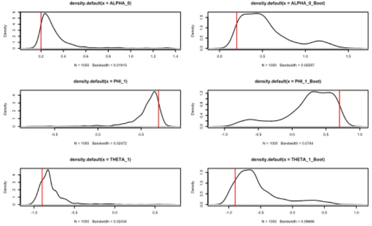
The aim of this section is to validate the bootstrap confidence intervals using simulation methods. We present one figure and one table for each model, the figure presents the estimated densities with a Monte Carlo simulation and bootstrap replication.

The objective of this comparison in to show that the bootstrap replicates, present similar densities than the Monte Carlo study. In other words, the Figures

(34)

Our study also presents the Tables2.1, 2.2 and 2.3where we get the results about the performance of the coverage using Moving Block Bootstrap (MBB) and asymptotic methods. We used 1000 bootstraps replications, 1000 different series.

0.0 0.5 1.0 1.5 2.0

0.0

0.5

1.0

1.5

2.0

density.default(x = ALPHA_0)

N = 1000 Bandwidth = 0.05271

D

ensi

ty

0.5 1.0 1.5 2.0 2.5

0.0

1.0

2.0

density.default(x = ALPHA_0_Boot)

N = 1000 Bandwidth = 0.04679

D

ensi

ty

-0.5 0.0 0.5 1.0

0.0

1.0

2.0

density.default(x = PHI_1)

N = 1000 Bandwidth = 0.04157

D

ensi

ty

-0.5 0.0 0.5

0.0

1.0

2.0

3.0

density.default(x = PHI_1_Boot)

N = 1000 Bandwidth = 0.03479

D

ensi

ty

-1.0 -0.5 0.0 0.5

0.0

1.0

2.0

density.default(x = THETA_1)

N = 1000 Bandwidth = 0.04935

D

ensi

ty

-1.0 -0.5 0.0 0.5 1.0

0.0

1.0

2.0

3.0

density.default(x = THETA_1_Boot)

N = 1000 Bandwidth = 0.04013

D

ensi

ty

Figure 2.1: Estimated densities with Monte Carlo and bootstrap negative binomial

Table 2.1: Negative Binomial GARMA(1,1) Confidence intervals n=100

Parameter Bootstrap Inferior Rejection Bootstrap Coverage Bootstrap Superior Rejection

β0 01.20% 98.80% 00.00%

φ1 00.00% 99.20% 00.80%

θ1 00.40% 99.60% 00.00%

Parameter Asymptotic Inferior Rejection Asymptotic Coverage Asymptotic Superior Rejection

β0 06.40% 89.70% 03.90%

φ1 03.80% 89.80% 06.40%

(35)

2.3 Simulation Study

0.2 0.4 0.6 0.8 1.0 1.2 1.4

0 1 2 3 4 5 6

N = 1000 Bandwidth = 0.01915

D

ensi

ty

0.0 0.5 1.0 1.5

0.0

0.5

1.0

1.5

N = 1000 Bandwidth = 0.05597

D

ensi

ty

-0.5 0.0 0.5

0

1

2

3

4

N = 1000 Bandwidth = 0.02472

D

ensi

ty

-1.0 -0.5 0.0 0.5 1.0

0.0

0.4

0.8

1.2

N = 1000 Bandwidth = 0.0744

D

ensi

ty

-1.0 -0.5 0.0 0.5

0

1

2

3

4

N = 1000 Bandwidth = 0.02434

D

ensi

ty

-1.0 -0.5 0.0 0.5 1.0

0.0

0.5

1.0

1.5

N = 1000 Bandwidth = 0.06666

D

ensi

ty

Figure 2.2: Estimated densities with Monte Carlo and bootstrap binomial

Table 2.2: Binomial GARMA(1,1) Confidence intervals n=100

β0 05.30% 94.70% 00.00%

φ1 00.00% 95.40% 04.60%

θ1 00.10% 99.90% 00.00%

β0 09.10% 90.00% 00.90%

φ1 00.90% 90.10% 09.00%

θ1 04.40% 90.60% 05.00%

0.5 1.0 1.5 2.0

0.0

1.0

2.0

N = 1000 Bandwidth = 0.04053

D

ensi

ty

0.0 0.5 1.0 1.5 2.0 2.5

0.0

0.5

1.0

1.5

2.0

N = 1000 Bandwidth = 0.05035

D

ensi

ty

-0.5 0.0 0.5

0.0

1.0

2.0

3.0

N = 1000 Bandwidth = 0.03033

D

ensi

ty

-0.5 0.0 0.5 1.0

0.0

1.0

2.0

3.0

N = 1000 Bandwidth = 0.03039

D

ensi

ty

-1.0 -0.5 0.0 0.5

0.0

1.0

2.0

3.0

N = 1000 Bandwidth = 0.03485

D

ensi

ty

-1.0 -0.5 0.0 0.5

0.0

1.0

2.0

3.0

N = 1000 Bandwidth = 0.02945

D

ensi

ty

Figure 2.3: Estimated densities with Monte Carlo and bootstrap Poisson

The Tables 2.1, 2.2 and 2.3 present the 95% coverage obtained using two

methods. The bootstrap coverage represents the 2.5% and 97.5% values of

(36)

present the values of95% coverage using the Gaussian confidence intervals, we

used the inverse of Fisher matrix to obtain the variances of the estimates and multiplied by₋1.96and1.96that represent the respective Gaussian value for95%.

The results of Tables 2.1, 2.2 and 2.3 clearly show the coverage obtained using the bootstrap confidence interval is higher than the coverage obtained using asymptotic confidence intervals. The results were verified for the binomial, negative binomial and Poisson GARMA models, which motivate the using of bootstrap methods to improve the confidence intervals.

We also present the Figures 2.1, 2.2 and 2.3 showing that the bootstrap replicates densities, in our results, are close than the Monte Carlo densities. In other words, the bootstrap method replicate the origina density of the parameters in the GARMA models, thus the bootstrap confidence intervals should represent a better option than the asymptotic ones.

Table 2.3: Poisson GARMA(1,1) Confidence intervals n=100

β0 00.10% 99.30% 00.60%

φ1 00.60% 99.40% 00.00%

θ1 00.00% 99.60% 00.40%

β0 05.00% 87.40% 07.60%

φ1 09.70% 82.00% 08.30%

θ1 10.20% 80.80% 09.00%

We can observe the clear improvement of the coverage using the MBB method. The strong asymmetry present on GARMA parameters impairs the quality of the asymptotic coverage. However, the MBB calibrates the confidence intervals to the asymmetric behavior, providing better estimates. There is a extensively discussion about the length of the block. We carried on different sizes of block, and also the random size using the geometric function. In our results we obtained better results following theLahiri(2003) assumptions about the block length to be betweenn14 ≤

b_≤n12.

2.4 Application to Real Data Sets

(37)

2.4 Application to Real Data Sets

2.4.1 Dengue Fever Real Data Analysis

We analyze the number of hospitalizations caused by dengue in Ribeirão Preto (São Paulo state) between January 2005 to December 2015.

Dengue disease is transmitted by several species of mosquito within thegenus Aedes, especially A.aegypti. The Aedes mosquito is easily identifiable by the

distinctive black and white stripes on its body. It prefers to breed in a clean and stagnant water. The summer months have higher volumes of rain, thus more clean and stagnant water is avaible. For Brazil this disease poses a significant public health problem. Therefore, analyzing this data helps healthcare institutions to prepare for possible outbreaks of dengue fever.

0 20 40 60 80 100 120

0 2000 4000 6000 8000 10000 12000 Months H o sp it a liza ti o n s ca u se d b y D e n g u e

Figure 2.4: Graph of Number of Hospitalizations caused by dengue

0 20 40 60 80 100

-0 .2 0.0 0.2 0.4 0.6 0.8 1.0 Lag AC F

Series y

0 20 40 60 80 100

-0 .2 0.0 0.2 0.4 0.6 Lag Pa rt ia l AC F

Series y

(38)

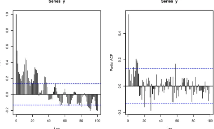
From Figure2.4and Figure2.5one clearly sees the seasonal component in the data. Therefore, we will add to the model two seasonal components, considering the period of 12 months. These components improve the model, linking the seasonal behavior to the number of hospitalizations caused by dengue.

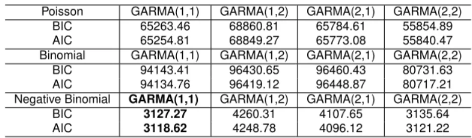
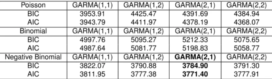
The Table2.4presented the values of BIC and AIC from different models and orders.

Table 2.4: Model Selection Criteria using Number of Hospitalizations caused by dengue

Poisson GARMA(1,1) GARMA(1,2) GARMA(2,1) GARMA(2,2)

BIC 65263.46 68860.81 65784.61 55854.89

AIC 65254.81 68849.27 65773.08 55840.47

Binomial GARMA(1,1) GARMA(1,2) GARMA(2,1) GARMA(2,2)

BIC 94143.41 96430.65 96460.43 80731.63

AIC 94134.76 96419.12 96448.87 80717.21

Negative Binomial GARMA(1,1) GARMA(1,2) GARMA(2,1) GARMA(2,2)

BIC 3127.27 4260.31 4107.65 3135.64

AIC 3118.62 4248.78 4096.12 3121.22

The extra parameter k was selected trying different values and analyzing

the likelihood value, 15 was the chosen value. The Moving Average parameter

θ1 present the 0 inside the confidence intervals, thus we go forward with the

GARMA(1,0) model with negative binomial. The Table 2.5 present the MLE estimate and the bootstrap confidence intervals in the GARMA model with the seasonality correction.

Table 2.5: Estimates of Hospitalizations caused by dengue series with GARMA(1,0) Negative Binomial

Parameter MLE estimate Lower Bootstrap Bound Upper Bootstrap Bound

β0 0.5517 0.5071 2.7321

βS₁ 0.6369 0.4288 0.9836

βS₂ 0.5763 0.4952 1.2413

φ1 0.9269 0.5787 0.9423

We evaluated the MLE results: CIβ0 = (0.3492,2.7543), CIβS₁ =

(0.3547,0.9192),CIβS₂ = (0.5055,1.6471) andCIφ1 = (0.4911,0.9628). Comparing

(39)

0 1 2 3 4

0.0 0.1 0.2 0.3 0.4 0.5 0.6

density.default(x = BETA_0)

N = 5000 Bandwidth = 0.1026

D

ensi

ty

0.2 0.4 0.6 0.8 1.0 1.2

0.0 0.5 1.0 1.5 2.0 2.5

density.default(x = BETA_0_Cos)

N = 5000 Bandwidth = 0.02321

D

ensi

ty

0.4 0.6 0.8 1.0 1.2 1.4 1.6

0.0

0.5

1.0

1.5

density.default(x = BETA_0_Sin)

N = 5000 Bandwidth = 0.03374

D

ensi

ty

0.4 0.5 0.6 0.7 0.8 0.9 1.0

0.0

1.0

2.0

3.0

N = 5000 Bandwidth = 0.01608

D

ensi

ty

Figure 2.6: Graph of bootstrap densities of each parameter

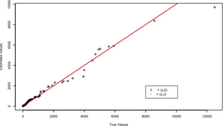
The Figure 2.7presents a quantile plot with the true values on x axis and the estimated values on y axis. The line represents the perfect model with real values on axis x and y.

0 2000 4000 6000 8000 10000 12000

0 2000 4000 6000 8000 10000 True Values Est ima te d Va lu e s o = (y,ŷ) = (y,y)

Figure 2.7: Adjusted values versus real values of Number of Hospitalizations caused by dengue

(40)

-6 -4 -2 0 2 4 6 0.00 0.05 0.10 0.15 0.20

density.default(x = Residuals)

N = 132 Bandwidth = 0.6279

D

ensi

ty

0 5 10 15 20

-0 .2 0.2 0.6 1.0 Lag AC F

Series Residuals

5 10 15 20

-0 .3 -0 .2 -0 .1 0.0 0.1 Lag Pa rt ial AC F

-2 -1 0 1 2

-5

0

5

Teorical Quantiles N(0,1)

R

esi

dual

s

Figure 2.8: Residual Analysis of Hospitalizations caused by dengue

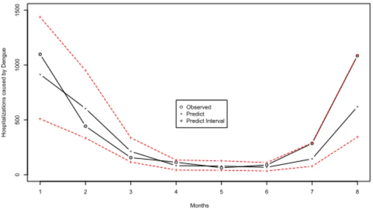
The 8 last values of the series were removed and fitted the model without them. Prediction one step ahead for 8 values was evaluated, thus the predicted value be compared with the true value.

1 2 3 4 5 6 7 8

0 500 1000 1500 Months H o sp it a liza ti o n s ca u se d b y D e n g u e * * * * * * * * + + + + + + + + + + + + + + + + o * + Observed Predict Predict Interval

Figure 2.9: Predictions with GARMA(1,0) Negative Binomial model with Hospitalizations caused by dengue series

The predictions are close to the real values, in some cases bigger than the real ones, in other lower than the real one, which indicates good predictions as we can see on Figure2.9. The confidence intervals for the predictions contain all the real values. The criterion MAPE, seeChen and Yang (2004), was calculated using the predictions given on Figure2.9. The value was30.17%which confirmed

(41)

2.4.2 Monthly Morbidity in S˜ao Paulo

We analyze the morbidity caused by external causes considering children younger than 1 year in São Paulo - Brazil. Morbidity represents the incidence or prevalence of a disease or of all diseases, we took observations between January of 1998 to December of 2015, containing 216 observations as we can see in Figure2.10.

0 50 100 150 200

100

120

140

160

180

200

Months

Mo

rb

ili

ty

in

Sa

o

Pa

u

lo

Figure 2.10: Graph of Morbidity in S˜ao Paulo

Figure 2.11 presents the autocorrelation function and the partial autocorrela-tion funcautocorrela-tion of Morbidity in São Paulo.

0 20 40 60 80 100

-0

.2

0.0

0.2

0.4

0.6

0.8

1.0

Lag

AC

F

Series y

0 20 40 60 80 100

-0

.2

0.0

0.2

0.4

Lag

Pa

rt

ia

l

AC

F

Series y

Figure 2.11: ACF and PACF for Morbidity in S˜ao Paulo

(42)

focussed in one of the most important states in Brazil.

We presented in this section three real data sets that will be adjusted in this work. We selected the first and the third one without seasonal component, that allows the using of the traditional moving block bootstrap. While, the second real data about dengue fever, presented seasonal component, requiring the use of periodic moving block bootstrapLe`skow and Synowiecki(2010).

The Table2.6presented the values of BIC and AIC from different models and orders.

Table 2.6: Model Selection Criteria using Monthly Morbidity in S˜ao Paulo

Poisson GARMA(1,1) GARMA(1,2) GARMA(2,1) GARMA(2,2)

BIC 3953.91 4425.47 4391.69 4384.94

AIC 3943.79 4411.97 4378.19 4368.07

Binomial GARMA(1,1) GARMA(1,2) GARMA(2,1) GARMA(2,2)

BIC 4997.76 5095.27 5212.33 5075.65

AIC 4987.64 5081.77 5198.83 5058.77

Negative Binomial GARMA(1,1) GARMA(1,2) GARMA(2,1) GARMA(2,2)

BIC 3822.07 3790.88 3784.90 3791.30

AIC 3811.95 3777.38 3771.40 3777.91

The extra parameter k was selected trying different values and analyzing

the likelihood value, 50 was the chosen value. The Moving Average parameter

θ1 also present the 0 inside the confidence intervals, thus we go forward

with the GARMA(2,0) model with negative binomial. Table 2.7 present the MLE estimates of the model GARMA(2,0) negative binomial with the respective bootstrap confidence intervals for each parameter.

Table 2.7: Estimates of Monthly Morbidity in S˜ao Paulo series with GARMA(2,0) negative binomial

Parameter MLE estimate Lower Bootstrap Bound Upper Bootstrap Bound

β0 0.8150 0.6958 2.5216

φ1 0.5620 0.3489 0.6764

φ2 0.2743 0.0271 0.4110

We evaluated the MLE confidence intervals: CIβ0 = (−0.0561,1.6863), CIφ1 =

(0.3803,0.7437) and CIφ2 = (0.0909,0.4578) Comparing with Table 2.7 we can

(43)

1 2 3 4

0.0

0.2

0.4

0.6

density.default(x = BETA_0)

N = 1001 Bandwidth = 0.1198

D

ensi

ty

0.2 0.3 0.4 0.5 0.6 0.7 0.8

0

1

2

3

4

5

N = 1001 Bandwidth = 0.01884

D

ensi

ty

-0.1 0.0 0.1 0.2 0.3 0.4 0.5

0

1

2

3

4

N = 1001 Bandwidth = 0.01993

D

ensi

ty

Figure 2.12: Graph of bootstrap densities of each parameter

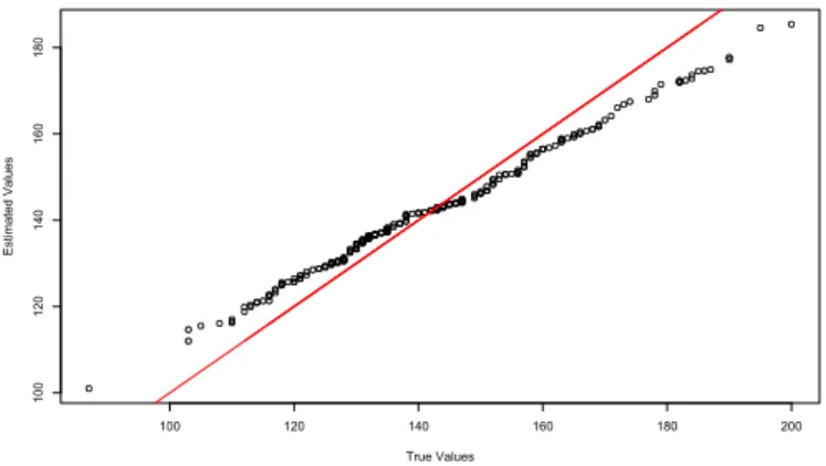
The Figure2.13presents a quantile plot with the true values on x axis and the estimated values on y axis. The line represents the perfect model with real values on axis x and y.

100 120 140 160 180 200

100

120

140

160

180

True Values

Est

ima

te

d

Va

lu

e

s

Figure 2.13: Adjusted values versus real values of Monthly Morbidity in S˜ao Paulo

(44)

-2 -1 0 1 2 3 0.0 0.1 0.2 0.3 0.4 0.5

density.default(x = Residuals)

N = 216 Bandwidth = 0.2205

D

ensi

ty

0 5 10 15 20

-0 .2 0.2 0.4 0.6 0.8 1.0 Lag AC F

5 10 15 20

-0 .2 -0 .1 0.0 0.1 0.2 Lag Pa rt ial AC F

-3 -2 -1 0 1 2 3

-3 -2 -1 0 1 2 3 4

Teorical Quantiles N(0,1)

R

esi

dual

s

Figure 2.14: Residual Analysis of Monthly Morbidity in S˜ao Paulo

The 8 last values of the series were removed and fitted the model without them. Prediction one step ahead for 8 values was evaluated, thus the predicted value be compared with the true value.

1 2 3 4 5 6 7 8

0 50 100 150 200 250 300 Months Mo rb ili ty in Sa o Pa u lo * * * * * * * * + + + + + + + + + + + + + + + + o * + Observed Predict Predict Interval

Figure 2.15: Predictions with GARMA(2,0) negative binomial model with Monthly Morbidity in S˜ao Paulo

The predictions are close to the real values, in some cases bigger than the real ones, in other lower than the real one, which indicates good predictions as we can see on Figure2.15. The confidence intervals for the predictions contain all the real values. The criterion MAPE, seeChen and Yang(2004), was calculated using the predictions given on Figure 2.15. The value was 10.20% which confirmed good

(45)

C

HAPTER

3 Bayesian GARMA Models for Count

Data

Abstract

Generalized autoregressive moving average (GARMA) models are a class of models that were developed for extending the univariate Gaussian ARMA time series model to a flexible observation-driven model for non-Gaussian time series data. This work presents Bayesian approach for GARMA models with Poisson, binomial and negative binomial distributions. A simulation study was carried out to investigate the performance of Bayesian estimation and Bayesian model selection criteria. Also three real datasets were analysed using the Bayesian approach on GARMA models.

3.1 Generalized Autoregressive Moving Average Model

The GARMA model, introduced by Benjamin et al. (2003), assumes that the conditional distribution of each observation yt, for t = 1, . . . , n given the

previous information set Ft−1 = (x1, . . . , xt−1, y1, . . . , yt−1, µ1, . . . , µt−1) belongs to

the exponential family. The conditional density is given by,

f(yt|Ft−1) = exp

ytαt−b(αt)

ϕ +d(yt, ϕ)

(46)

whereαt e ϕ are conical and scale parameter respectively, with b(·)e d(·) being specific functions that define the particular exponential family. The conditional mean and conditional variance ofyt given Ft−1 is represented by the terms µt =

E(yt|Ft−1) =b′(αt)andV ar(yt|Ft−1) =ϕb′′(αt), witht= 1, . . . , n.

Just as in Generalized Linear Models (GLM,McCullagh and Nelder(1989)),µt,

is related to the linear predictor,ηt, by a twice-differentiable one-to-one monotonic link functiong(_·). The linear predictor for the GARMA model is given by,

g(µt) = ηt =x′tβ+ p X

j=1

φj{g(yt−j)−x′t−jβ}+ q X

j=1

θj{g(yt−j)−ηt−j}. (3.2)

The GARMA(p,q) model is defined by equations (3.1) and (3.2). For certain

functions g, it may be necessary to replace yt with yt∗ in (3.2) to avoid the non-existence ofg(yt) for certain values ofyt. The form y∗t depends on the particular functiong(.)and is defined for specific cases later.

The definition of GARMA model allows to consider the adjust of exogenous variablesx′

t however in this work the termx′tβwill be considered as a constantβ0.

For count data time series we will consider the following distributions.

3.1.1 Poisson GARMA model

Suppose thatyt|Ft−1 follows a Poisson distribution with meanµt. Then,

f(yt|Ft−1) = exp{ytlog(µt)−µt−log(yt!)}. (3.3) and Yt|Ft−1 has distribution in the exponential family with ϕ = 1, αt = log(µt),

b(αt) = exp(αt),c(yt, ϕ) = −log(yt!)andν(µt) = µt. The canonical link function for this model is the logarithmic function, so that the linear predictor is given by,

log(µt) =β0+

p X

j=1

φj{logyt∗−j}+ q X

j=1

θj{log(yt∗−j)−log(µt−j)}, (3.4)

Wherey∗

t−j = max(yt−j, c),0 < c < 1. The Poisson GARMA model is defined by equations (3.3) and (3.5).

3.1.2 Binomial GARMA model

Suppose thatyt|Ft−1 follows a binomial distribution with meanµt. Then,

f(yt|Ft₋1) = exp

ytlog

µt

m−µt

+mlog

m₋µt

m

+ log

Γ(m+ 1)

Γ(yt+ 1)Γ(m−yt+ 1)

(47)

3.1 Generalized Autoregressive Moving Average Model

The canonical link function for this model is the logarithmic function. The linear predictor is given by,

log

µt

m₋µt

=β0+

p X

j=1

θj{log(yt∗−j)−log(µt−j)}, (3.5)

withy∗

t−j = max(yt−j, c),0< c <1, andmis known.

3.1.3 Negative Binomial

Letyt a time series such thatyt|Ft−1 ∼N B(k, µt). Then,

f(yt|Ft−1) = exp

klog

k µt+k

+ytlog

µt

µt+k

+ log

Γ(k+yt)

Γ(yt+ 1)Γ(k)

,

which belongs to the exponential family with k known. The link function for this

model is the logarithmic function

log

k µt+k

=β0+

p X

j=1

θj{log(yt∗−j)−log(µt−j)},

withy∗

t−j = max(yt−j, c),0< c <1.

3.2 Bayesian Approach on GARMA Models

3.2.1 Defining the Prior Densities

Using the logarithmic in link function to guarantee positive values for any values of the vectorsβ = (β1, . . . , βm),Φ = (φ1, . . . , φp)andΘ = (θ1, . . . , θq).β,φi. Thus, a multivariate Gaussian prior will be proposed for each parameter.

β _∼ N(µ0, σ₀2I0),

Φ _∼ N(µ1, σ₁2I1) Θ _∼ N(µ2, σ₂2I2)

where µ0,µ1,µ1 are vectors with length m, p and q respectively, σ2

0, σ21 and σ12

represent the prior variance andI0,I1 andI2 arem_×m,p_×pandq_×q identity

(48)

hyper parameters, when there is no prior knowledge on these parameters it can be considered a vary large variance making the prior densities flats. The partial likelihood function for GARMA models can be constructed as follows

L(β,Φ,Θ_|Y) _∝

n Y

t=r+1

f(yt|Ft−1)

∝

n Y

t=r+1

exp

ytαt−b(αt)

ϕ +d(yt, ϕ)

,

whereαt=g(µt), which represent the link function given by

g(µt) =x′tβ+ p X

j=1

φj{g(yt∗−j)−x′t−j}+ q X

j=1

θj{g(yt∗−j)−g(µt−j)},

for allt=r+ 1, . . . , n.

The posterior density is obtained combining the likelihood function with the prior densities. Let the vectorY = (yt, yt−1, . . . , y1, xt, xt−1, . . . , x1, . . .) represent

the necessary information to construct the likelihood function. The posterior density is then given by,

π(β,Φ,Θ_|Y)_∝L(β,Φ,Θ_|Y)π0(β,Φ,Θ). (3.6)

However, the joint posterior density of parameters in the GARMA models can not be obtained in closed form. Therefore, Markov chain Monte Carlo (MCMC) sampling strategies will be employed for obtaining samples from this joint posterior distribution. In particular, we use a Metropolis-Hastings algorithm to yield the required realisations. We adopt a sampling scheme where the parameters are updated as o single block and at each iteration we generate new values from a multivariate normal distribution centred around the maximum likelihood estimates with a variance-covariance proposal matrix given by the inverse Hessian evaluated at the posterior mode.

3.2.2 Bayesian prediction for GARMA models

(49)

3.2 Bayesian Approach on GARMA Models

values of the informationyt+h,h≥1, when all the information available is until time

t. To evaluate this forecasting is necessary to find the predictive density function p(yt+h|Y).

Denoting the information set bFt+h = (bxt+h, . . . , xt, xt−1, . . . , ybt+h−1, . . . , yt,

yt−1, . . . µbt+h−1,. . . , µt, µt−1, . . .), where byt+h−i = yt+h−i, if h ≤ i, else ybt+h−i =

E_{yt+h−i|bFt+h−i}, i = 1,2, . . . h+ 1. The general idea is that Fbt+h contains all the data observed until the time t, for the future time t+h, h _≥ 1, the set Fbt+h is completed with forecasts of necessary information to estimateyt+h. Starting with,

f(yt+h|β,Φ,Θ,bFt+h) = exp

yt+hαt+h−b(αt+h)

ϕ +d(yt+h, ϕ)

, (3.7)

The conditional mean and variance of yt+h given bFt+h is represented by the terms µ_bt+h = E(yt+h|bFt+h) = b′(αt+h) and V ar(yt+h|Ft+h) = ϕb′′(αt+h). The µt+h,

is related to the predictor,ηt+h, by a twice-differentiable one-to-one monotonic link functiong(_·). The linear predictor for the GARMA model is given by,

g(µt+h) = ηt+h =xb′t+hβ+ p X

j=1

φj{g(ybt+h−j)−xb′t+h−jβ}+ q X

j=1

θj{g(ybt+h−j)−ηbt+h−j}. (3.8) With the equation (3.7) and posterior density (3.6), the predictive density for

yt+h can be written as,

p(yt+h|Fbt+h) = Z

{β,Φ,Θ}∈Ω

f(yt+h|β,Φ,Θ,Fbt+h)π(β,Φ,Θ|Y)dβdΦdΘ.

The aim is determine the predictive density using the MCMC algorithm, thus

b

p(yt+h|bFt+h) =

1

Q

Q X

j=1

f(yt+h|β(j),Φ(j),Θ(j),Fbt+h). (3.9)

Given the predictive density, the next step is to evaluate the prediction

E(yt+h|Fbt+h) = ˆyt+h.

E(yt+h|Fbt+h) = Z

yt+h∈R

(50)

Substituting the equation (3.9) the equation (3.10) can be rewritten by,

E(yt+h|bFt+h) = Z

yt+h∈R

yt+h Z

{β,Φ,Θ}∈Ω

f(yt+h|β,Φ,Θ,bFt+h)π(β,Φ,Θ|Y)dβdΦdΘ

dyt+h.

Using properties of integer, we can rewrite (3.11) as,

E(yt+h|Fbt+h) = Z

{β,Φ,Θ}∈Ω

"Z

yt+h∈R

yt+hf(yt+h|β,Φ,Θ,Fbt+h)dyt+h #

π(β,Φ,Θ_|Y)dβdΦdΘ.

The equation (3.11) represent

E(yt+h|Fbt+h) = Z

{β,Φ,Θ}∈Ω

h

E(yt+h|β,Φ,Θ,bFt+h) i

π(β,Φ,Θ_|Y)dβdΦdΘ. (3.11)

Denoting by µt+h(β,Φ,Θ,bFt+h) = E(yt+h|β,Φ,Θ,Fbt+h). Hence, using the MCMC vector (β(j),Φ(j)_,_Θ(j)₎_, _j _{= 1}_,₂_{, . . . , Q}_{, the} _E₍_y

t+h|Fbt+h)can be estimated by

b

yt+h =

1

Q

Q X

k=1

µt+h(β(k),Φ(k),Θ(k),bFt+h), (3.12)

where

g(µ(_tk₊)_h) = xb′

t+hβ(k)+ p X

j=1

φ(_jk)_{g(y_bt+h−j)−xb′t+h−jβ(k)}+ q X

j=1

θ(_jk)_{g(_byt+h−j)−ηb(_t₊k)_h₋_j}. (3.13) Credible intervals for _byt+h can be calculated using the 100α%, and 100(1 −

α)% quantiles of the MCMC sample µ(_t₊k)_h, with k = 1, . . . , Q. An approach to

estimate the credible interval of _byt+h is the Highest Posterior Density (HPD), see

(51)

3.2 Bayesian Approach on GARMA Models

A100(1₋α)%HPD region fory_bt+h are a subset C ∈ Rdefined byC = {yt+h :

p(yt+h|Fbt+h)≥κ}, whereκis the largest number such that Z

yt+h≥κ

p(yt+h|Fbt+h)dyt+h = 1−α. (3.14)

We can use thep_b(yt+h|bFt+h)MCMC estimates, given by the equation (3.9), to estimate the100(1₋α)%HPD region. The next section contains all the Bayesian

simulation study. Metrics were used to verify the quality and performance of the adjust.

3.2.3 Algorithm used to calculate the

CI

(1−δ)

for predictions

1. Let a sequence of forecast values_byt+h forh= 1, . . . , H.

2. Takeh= 1,k = 0,y_t(0)₊_h = 0,S_t(0)₊_h = 0 and also initiateLB = 0,U B=0.

3. Using the initial values evaluate the equation:

f(y(_t₊k)_h_|β(j),Φ(j),Θ(j),Fbt+h) = exp

y_t(₊k)_hα_t(₊j)_h₋b(α_t(j₊)_h)

ϕ +d(y

(k)

t+h, ϕ) !

,

and also,

b

p(y_t(₊k)_h_|Fbt+h) =

1

Q

Q X

j=1

f(y(_t₊k)_h_|β(j),Φ(j),Θ(j),Fbt+h).

4. Usingp_b(y_t(₊k)_h_|Fbt+h)computeSt(+k+1)h with

S_t(₊k+1)_h =S_t(₊k)_h+p_b(y_t(₊k)_h_|Fbt+h)

5. IfLB = 0andS_t(₊k+1)_h _≥δ,_→yt+h,δ =y(t+k)h andLB = 1.

6. IfU B = 0 andS_t(₊k+1)_h _≤(1₋δ),_→yt+h,(1−δ) =yt(+k)h andU B = 1.

7. IfLB = 0 or U B = 0, take k = k+ 1 and y_t(₊k)_h = y_t(₊k−_h1) + 1, repeat steps 3

and 4 untilLB = 1 andU B = 1.

The percentiles100δ%and100(1₋δ)%are represented byyt+h,δ andyt+h,(1−δ)

(52)

yt+h,δ = max (

y_t(₊r)_h

r X

k=1

b

p(y(_t₊k)_hbFt+h)≤δ )

.

yt+h,(1−δ)= min

(

y_t(₊r)_h

r X

k=1

b

p(y_t(₊k)_hbFt+h)≥(1−δ) )

.

The confidence interval100(1₋δ)%for the predictions is given by:

CI(1−δ) =yt+h,δ;yt+h,(1−δ)

The next section contains all the Bayesian simulation study. Metrics were used to verify the quality and performance of the adjust.

3.3 Simulation Study

In this section we conduct a simulation study for negative binomial GARMA(p, q) models with different orders p and q. The actual parameter values

used to simulate the artificial series are shown in Table 3.1 and the parameter

k of the negative binomial was fixed at k = 15. These values were chosen

taking into account that a GARMA model can be nonstationary since they are in the exponencial family and the variance function depends on the mean. So, we opted to chose parameter values that would generate moderate values for the time series. The experiment was replicated m = 1000 times for each model.

For each dataset we used the prior distributions as described in Section 5.2

with mean zero and variance 200. We then drew samples from the posterior distribution discarding the first 1000 draws as burn-in and keeping every 3rd sampled value resulting in a final sample of 5000 values. All the computations were implemented using the open-source statistical software language and environmentRR Development Core Team(2010).

Table 3.1: Parameters values to simulate from Negative Binomial GARMA(p,q).

Order β0 φ1 φ2 θ1 θ2

(1,1) 0.80 0.50 - 0.30

-(1,2) 1.00 0.30 - 0.40 0.25

(2,1) 0.55 0.30 0.40 0.20

-(2,2) 0.65 0.30 0.40 0.25 0.35

(53)

3.3 Simulation Study

acceptance rates in the MCMC algorithm called Acceptance Probabilities (AP). These metrics are defined as,

CB = 1

m

m X

i=1

θ₋θˆ(i)

θ

,

CE2 = 1

V ar

1

m

m X

i=1

(ˆθ(i)₋θ)2

AP = 1

m

m X

i=1

ˆ

r(i),

where_θˆ(i) _and_r_ˆ(i) _{are the estimate of parameter}_θ _{and the computed acceptance}

rate respectively for the i-th replication, i = 1, . . . , m. In this paper we take

the posterior means of θ as point estimates. Also, the variance term (V ar) that

appears in the definition of CE is the sample variance of_θˆ(1)_{, . . . ,}_θˆ(m)_.

The estimation results appear in Table 3.2 where the posterior mean and variance (in brackets) as well as the aforementioned metrics are shown for each model and parameter. These results indicate good properties with relatively small values of the corrected bias (CB), values of the corrected error (CE) around 1 and acceptance probabilities between 0.20 and 0.70.

We also include Table 3.3 with the proportions of correct model choice using three popular Bayesian model selection criteria. Specifically, we adopt the expected Bayesian information criterion (EBIC, Carlin and Louis (2001)), the Deviance information criterion (DIC, Spiegelhalter et al. (2002)) and the conditional predictive ordinate (CPO,Gelfand et al. (1992)) to select the order of the GARMA models. Each column in this table contains the model order and the associated proportions of correct model choice according to EBIC, DIC and CPO criteria. Higher proportions of correct model choices are observed as the sample sizes increase for all models and criteria. Also, EBIC and CPO tend to perform better for GARMA(1,1) and GARMA(1,2) models but none performed particularly well with GARMA(2,2) models.

Finally, this simulation study was carried out also for the Poisson and binomial distributions with results similar to the ones shown. These results are not included to save space.

3.4 Bayesian Real Data Analysis

(54)

Table 3.2: Monte Carlo experiments. Corrected bias, corrected errors and mean acceptance rates

for the Bayesian estimation of Negative Binomial GARMA(p,q) model.

Parameter Mean(Var)(1,1) CB(1,1) CE(1,1) AP(1,1) Mean(Var)(1,2) CB(1,2) CE(1,2) AP(1,2)

β0 0.8571(0.0065) 0.0984 1.2247 0.3746 1.0823(0.0196) 0.1276 1.1592 0.3182

φ1 0.4695(0.0026) 0.0947 1.1637 0.3511 0.2554(0.0097) 0.2820 1.0965 0.2702

φ2 - - -

-θ1 0.2927(0.0033) 0.1531 1.0071 0.6480 0.4099(0.0091) 0.1900 1.0048 0.4327

θ2 - - - - 0.2478(0.0037) 0.1929 1.0001 0.5882

Parameter Mean(Var)(2,1) CB(2,1) CE(2,1) AP(2,1) Mean(Var)(2,2) CB(2,2) CE(2,2) AP(2,2)

β0 0.6198(0.0097) 0.1740 1.2240 0.2786 0.7344(0.0079) 0.1497 1.3171 0.3397

φ1 0.2798(0.0152) 0.3295 1.0127 0.1422 0.2887(0.0054) 0.1959 1.0111 0.2282

φ2 0.3794(0.0066) 0.1661 1.0307 0.2091 0.3414(0.0049) 0.1485 1.0787 0.2348

θ1 0.2012(0.0182) 0.5334 0.9995 0.3214 0.2430(0.0052) 0.2307 1.0040 0.5237

θ2 - - - - 0.3464(0.0027) 0.1193 1.0017 0.6614

Table 3.3: Proportions of correct model chosen via Bayesian criteria with Negative Binomial

GARMA(p,q) models.

EBIC

Size GARMA(1,1) GARMA(1,2) GARMA(2,1) GARMA(2,2)

200 0.9379 0.3042 0.5626 0.4450

500 0.9799 0.6156 0.8048 0.5825

1000 0.9852 0.9039 0.8471 0.6772

DIC

200 0.6316 0.4804 0.5445 0.4437

500 0.6876 0.6476 0.6221 0.4925

1000 0.7155 0.7364 0.6469 0.7154

CPO

200 0.8078 0.3493 0.5575 0.4112

500 0.8188 0.5925 0.5993 0.4625

1000 0.8325 0.7266 0.6152 0.7317

varying orders and computed the Bayesian selection criteria EBIC, DIC and CPO for model comparison. In all cases we used the diagnostic proposed byGeweke

(1992) to assess convergence of the chains. This is based on a test for equality of the means of the first and last part of the chain (by default the first 10%and the

last 50%). If the samples are drawn from the stationary distribution, the two means

GARMA models, a new perspective using Bayesian methods and transformations

GARMA models, a new perspective using

Bayesian methods and transformations

GARMA models, a new perspective using Bayesian methods and

transformations

Modelos GARMA, uma nova perspectiva usando métodos

Bayesianos e transformações.

Agradecimentos

Abstract

Resumo

Contents

List of Figures

List of Tables

C

HAPTER

1

Introduction

C

HAPTER

2

GARMA models and moving block

bootstrap

Abstract

2.1 Generalized Autoregressive Moving Average (GARMA)

model

2.1.1 Model Definition

2.1.2 Poisson GARMA model

2.1.3 Binomial GARMA model

2.1.4 Negative Binomial

2.1.5 Seasonal Component

2.1.6 Maximum Likelihood Estimation and Inference

2.1.7 Predictions with GARMA models

2.2 Resampling methods

2.2.1 Moving Block Bootstrap

2.3 Simulation Study

2.4 Application to Real Data Sets

2.4.1 Dengue Fever Real Data Analysis

2.4.2 Monthly Morbidity in S˜ao Paulo

C

HAPTER

3

Bayesian GARMA Models for Count

Data

Abstract

3.1 Generalized Autoregressive Moving Average Model

3.1.1 Poisson GARMA model

3.1.2 Binomial GARMA model

3.1.3 Negative Binomial

3.2 Bayesian Approach on GARMA Models

3.2.1 Defining the Prior Densities

3.2.2 Bayesian prediction for GARMA models

3.2.3 Algorithm used to calculate the

CI

for predictions

3.3 Simulation Study

3.4 Bayesian Real Data Analysis