http://dx.doi.org/10.1590/0104-530X2359-15
Resumo: Neste trabalho, aborda-se o problema de roteamento de veículos com janelas de tempo e múltiplos entregadores, uma variante do problema de roteamento de veículos que, além das decisões de programação e roteamento dos veículos, envolve a determinação do tamanho da tripulação de cada veículo de entrega. Esse problema surge na distribuição de bens em centros urbanos congestionados em que, devido aos tempos de serviço relativamente longos, pode ser difícil atender todos os clientes durante o horário de trabalho permitido. Diante dessa diiculdade, uma alternativa consiste em incluir a designação de entregadores adicionais para reduzir os tempos de serviço, o que gera custos adicionais aos custos tradicionais de deslocamento e utilização de veículos. Dessa forma, o objetivo é deinir rotas para atender grupos de clientes, minimizando o número de veículos usados, o número de entregadores designados e a distância total percorrida. Para tratar o problema são propostas duas abordagens metaheurísticas baseadas em Busca Local Iterada e Busca em Vizinhança Grande. O desempenho das abordagens propostas é testado utilizando conjuntos de instâncias disponíveis na literatura.
Palavras-chave: Roteamento de veículos; Múltiplos entregadores; Busca Local Iterada; Busca em Vizinhança Grande. Abstract: This paper addresses the vehicle routing problem with time windows and multiple deliverymen, a variant of the vehicle routing problem which includes the decision of the crew size of each delivery vehicle, besides the usual scheduling and routing decisions. This problem arises in the distribution of goods in congested urban areas where, due to the relatively long service times, it may be dificult to serve all customers within regular working hours. Given this dificulty, an alternative consists in resorting to additional deliverymen to reduce the service times, which typically leads to extra costs in addition to travel and vehicle usage costs. The objective is to deine routes for serving clusters of customers, while minimizing the number of routes, the total number of assigned deliverymen, and the distance traveled. Two metaheuristic approaches based on Iterated Local Search and Large Neighborhood Search are proposed to solve this problem. The performance of the approaches is evaluated using sets of instances from the literature.
Keywords: Vehicle routing; Multiple deliverymen; Iterated Local Search; Large Neighborhood Search.
Metaheuristic approaches for the vehicle routing
problem with time windows and multiple deliverymen
Abordagens metaheurísticas para o problema de roteamento de veículos com janelas de tempo e múltiplos entregadores
Aldair Álvarez1 Pedro Munari1
1 Departamento de Engenharia de Produção, Universidade Federal de São Carlos – UFSCar, Rod. Washington Luiz, Km 235, CEP 13565-905, São Carlos, SP, Brazil, e-mail: [email protected]; [email protected]
Received June 23, 2015 - Accepted Dec. 28, 2015 Financial support: CAPES, FAPESP, CNPq.
1 Introduction
Transportation processes are involved in multiple ways in production systems, especially in those involving distribution activities. Such processes can have a huge impact on competitiveness and on service levels of industries. For example, transportation
processes may represent up to 20% of the inal costs
of goods produced by a company (Toth & Vigo, 2002). In addition, it is estimated that distribution costs can represent up to 75% of logistics costs of an organization
(Bräysy & Gendreau, 2005), making it necessary to make efforts for the improvement of those processes.
Amongst the distribution activities, arises the vehicle routing problem (VRP), a challenging problem that
is faced daily by many companies dealing with the transportation of goods or people. In practice, the VRP plays an important role in distribution systems and,
therefore, solving this problem is a key activity for eficient operations management in the companies.
soft drinks, dairy and beer companies which must
replenish on a regular basis (daily or every few days)
small and medium establishments like convenience
stores, restaurants, grocery stores, among others. These establishments are typically located in very
busy areas, in which it becomes dificult to park the delivery trucks. Thus, the vehicles park in a strategic
point of a region having a group of customers and the deliveries are made on foot to these customers
by the service workers of the route. By making the
deliveries in this way, the service time in the group of customers (from now on, cluster of customers) can be relatively long when compared with travel times,
which may dificult serving all customers during regular working hours. In these contexts, the use of additional
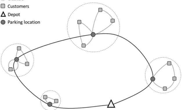
deliverymen becomes an important feature as it can speed up the delivery of the products, reducing the service time in each cluster. An example of a typical route in the VRPMD is shown in Figure 1, where deliveries are performed in two phases. First, the
truck arrives to the parking location of each cluster, then the service workers have to go on foot from the parking location to each customer in the cluster.
In spite of the theoretical and practical importance of this variant, there are few researches on the VRPMD in the literature, which encourages the development of solution methods for it. In this paper, we propose two metaheuristic approaches for the Vehicle Routing Problem with Time Windows and Multiple Deliverymen, which are based on Iterated
Local Search (ILS) and Large Neighborhood Search (LNS). These metaheuristics have been successfully applied to solve different variants of the VRP, e.g.,
VRP with heterogeneous leet (Subramanian et al., 2012); VRP with time windows (Pisinger & Ropke,
2007); Dynamic VRP (Hong, 2012); VRP with multiple routes (Azi et al., 2014); VRP with split
deliveries (Silva et al., 2015); and VRP with pickup and deliveries (Ropke & Pisinger, 2006). Thus, we
believe that ILS and LNS can also be effective for the problem addressed in this research. Using instances from the literature, we compare the performance of the two proposed metaheuristic approaches between themselves, as well as we compare their performances with other methods proposed in the literature.
The remainder of this paper is organized as follows. In Section 2, we describe the problem to be addressed. Section 3 presents the metaheuristic approaches proposed to solve the problem. Next, we show the results of computational experiments in Section 4. Finally, Section 5 highlights general conclusions of this research and the plans for future research.
2 Problem statement
In this article, we address the vehicle routing problem with time windows and multiple deliverymen (VRPTWMD), a variant of the classic VRP with time windows that considers the crew size in the vehicles as a decision, in addition to routing and scheduling decisions. In the VRPTWMD, service times can be
very long when compared to travel times because in the problem we must serve clusters of customer instead of serving individual customers. Furthermore, service times depend on the number of deliverymen assigned to the delivery route.
In practical terms, the problem involves two stages:
irst, the customers must be clustered around parking
locations; then, routes must be designed to visit the
deined clusters. Vehicle capacity, time windows and available deliverymen constraints must be satisied
while the total cost is minimized (vehicle usage, deliverymen assignment and traveled distance costs). Nevertheless, given the complexity of the complete problem, clustering and routing stages are addressed separately (Senarclens de Grancy & Reimann, 2014). Therefore, regarding the VRPTWMD, it is assumed that the clustering stage is performed in advance,
thus each cluster has its predeined parking location,
cumulated demand and service time, which includes
the transportation of the goods from the parking
location to the customers of the cluster.
After describing the context above, the VRPTWMD can be formally stated as follows. Given a homogeneous
leet of vehicles located in a central depot, each one
with capacity Q, it must be used to visit n clusters, aiming to serve its demands d ii, 1,= …,n. The objective
is to deine a set of minimum cost routes, satisfying
the following constraints: each cluster must be visited exactly once and within its time window w wia, bi, i.e., the vehicle must serve the cluster before the time instant b
i
w and must wait until the time instant a i
w to start serving the cluster, if the vehicle arrives before this time. The service time in cluster i for a route with
l deliverymen is known in advance and denoted by
il
s . The travel time between clusters i and j is given by tij. The vehicles are required to come back to the
depot at the end of their trips.
The cost of a solution S is deined by Equation 1,
where V denotes the number of vehicles used,
E denotes the total number of deliverymen assigned and D denotes the total traveled distance. Constants
p1, p2 and p3 denote the weights of each objective, which are used to impose priority over them.
( ) 1 2 3
c S =p V+p E+p D (1)
In order to show how the use of additional deliverymen may improve the service levels, consider the next
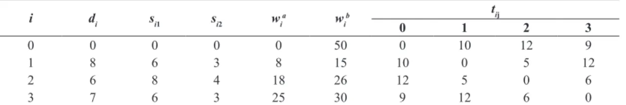
illustrative example with three clusters, a vehicle with a capacity large enough to serve all clusters and the data of Table 1. In the table, , , , , 1 2
a b i i i i i
d s s w w
denote the demand, the service times with one and two deliverymen and the time window of cluster i, respectively. Cluster i = 0 represents the depot. Solutions for the problem in Table 1, considering routes with one and two deliverymen are presented in Figure 2. In the igure, wi represents the service start time in cluster i. Note that in the route with two deliverymen (left), all clusters can be served within the planning horizon (latest arrival time at the depot). On the other hand, the route with one deliveryman (right) cannot serve cluster 3 because, departing from cluster 2, it is not possible to arrive in cluster 3 before its latest arrival time ( 3
b
w).
3 Metaheuristic approaches
In this section, we describe the metaheuristic approaches developed to solve the VRPTWMD.
The irst approach is based on the metaheuristic
ILS and it is presented in Section 3.2. The second approach is based on the metaheuristic LNS and its description is shown in Section 3.3. Both approaches use the same constructive heuristic, which is described in Section 3.1.
3.1 Constructive heuristic
To generate an initial solution for the metaheuristic approaches, we developed a constructive heuristic similar to the used by Senarclens de Grancy & Reimann (2014), which is based on the classic Solomon’s insertion heuristic I1 (Solomon, 1987). In our implementation, routes are constructed sequentially, starting with the farthest unrouted cluster and using the maximum possible number of deliverymen on the vehicle. Next, clusters are inserted in the current route minimizing a weighted sum of additional time and distance when the cluster is inserted into the route. When no more clusters can be inserted into the route, a new one is initialized and the process is repeated until a solution serving all clusters is reached.
3.2 ILS-based metaheuristic approach
Table 1. Data for a VRP with multiple deliverymen.
i di si1 si2 wia w
i
b tij
0 1 2 3
0 0 0 0 0 50 0 10 12 9
1 8 6 3 8 15 10 0 5 12
2 6 8 4 18 26 12 5 0 6
The irst developed approach is based on ILS
(Lourenço et al., 2003), a metaheuristic that applies a local search repeatedly to a set of solutions obtained by perturbing previously visited local optimal solutions. An ILS algorithm uses four basic components: (i) an initial solution; (ii) a local search procedure; (iii) a perturbation mechanism; and (iv) an acceptance criterion. For further information on ILS algorithms, see Lourenço et al. (2010).
In addition to the usual components of an ILS metaheuristic, the proposed approach uses two additional heuristics to enhance its performance, namely, deliverymen reduction heuristic and route
reduction heuristic, which are speciically designed
for the VRPTWMD. The overall structure of this approach is shown in Figure 3. First, an initial solution is generated with the constructive heuristic (line 2). This solution is improved through the local search
heuristic and deined as the best initial solution in
each iteration of the approach (line 5). The main loop of the algorithm is given on lines 7 to 23 and aims at improving the current best solution using the local search procedure (line 9) combined with the deliverymen reduction heuristic (line 10) and the perturbation mechanism (line 8). The acceptance
criterion deines that the perturbation is performed on
the incumbent solution of the current iteration of the approach (S+). The main loop comprises two phases, each one of them terminates when the algorithm reaches MaxIterILS consecutive perturbations without improvements (lines 13-15 and 16-18, respectively). Then, the best global solution is updated (lines 24-26) and a new main loop is started, in case that the overall stopping criterion has not been reached.
The two phases of the approach are needed to consider different parts of the objective function of
the VRPTWMD. The irst phase focuses on reducing
the number of vehicles used in the solutions. For this,
the perturbation is performed with the route reduction heuristic of Section 3.2.3. The second phase of the approach focuses on reducing the traveled distance and therefore it uses the perturbation procedure of
Section 3.2.2. Note that in the irst phase the route
reduction heuristic not always obtain a different solution. In these cases, the perturbation procedure of the second phase is applied. Finally, also note that
Figure 2. (left) Solution with two deliverymen in the route; (right) Solution with one deliveryman in the route.
the reduction of the number of deliverymen is directly addressed in the approach by using the deliverymen reduction heuristic.
3.2.1 Local search
The local search procedure plays the role of the
intensiication tool in ILS. In our approach, the
local search procedure is a variable neighborhood descent heuristic (Mladenovic & Hansen, 1997) with random neighborhood ordering (RVND). This heuristic applies a set of neighborhood structures (local search operators) to progressively improve the solution. First, a set of neighborhood structures
{
1}
, , nV= v …v , is initialized. While V is not empty, a neighborhood structure i
v is chosen at random and applied to the solution. In case of improvement, V
is reestablished to its initial form (containing all the neighborhood structures). Otherwise, i
v is deleted of the set. Infeasible solutions are forbidden and the
irst improvement strategy is adopted. Moreover, to
reinforce the RVND heuristic, the route reduction heuristic is applied when one neighborhood structure improves the solution. The set of used neighborhood structures contains the following movements:
• Inter-routes neighborhood structures:
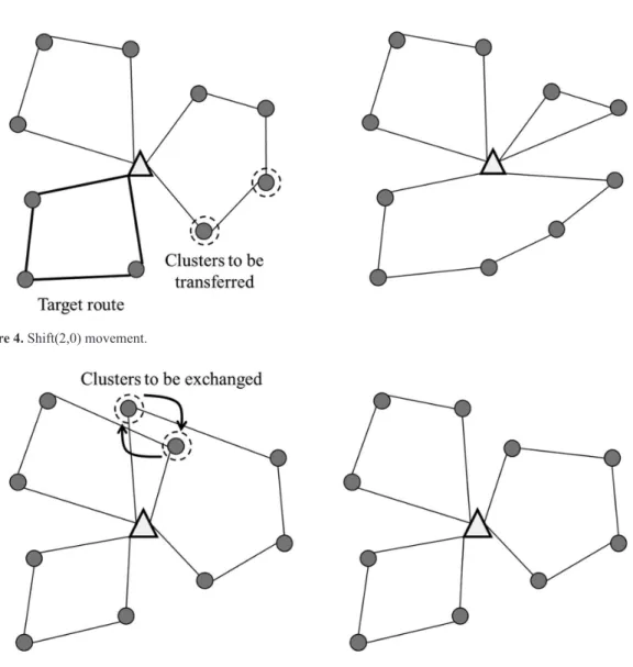
o Shift(k,0): move k adjacent clusters from route r1 to route r2, k={1, 2, 3} (see Figure 4).
o Swap(1,1): exchange cluster c1 of route r1
with cluster c2 of route r2 (see Figure 5).
o Swap(2,1): exchange two adjacent clusters c1
and c2 of route r1 with cluster c3 of route r2.
o Swap(2,2): exchange two adjacent clusters c1
and c2 of route r1 with two adjacent clusters
c3 and c4 of route r2.
• Intra-routes neighborhood structures:
Figure 4. Shift(2,0) movement.
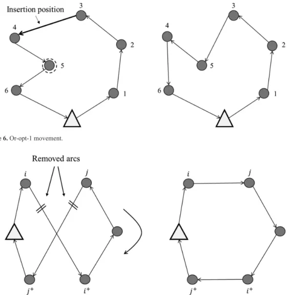
o Or-opt-1: move one cluster from its current position to another one in the same route (see Figure 6).
o 2-opt: two nonadjacent arcs (i, i+) and (j, j+)
are removed and another two arcs (i, j) and (i+, j+) are added in such a way that a new
route is generated (see Figure 7).
3.2.2 Removal and insertion heuristic
The perturbation mechanism is responsible for the
diversiication in the ILS since it changes the current
local optimal solution. In our ILS approach, one perturbation mechanism consists of one operation of removal and relocation of a set of clusters, based on
the procedure of Melechovsky (2012). For a given
route, up to nP cluster nodes are randomly selected and removed from the route. Each removed cluster is then tested for a feasible insertion into the remaining routes
of the solution. If such feasible insertion exists, the cluster is relocated to its new position. If some of the clusters cannot be inserted, a new single route with the maximum possible crew is created for serving them.
3.2.3 Route reduction heuristic
Given that reducing the number of routes can also reduce the number of allocated deliverymen, the route reduction heuristic of Senarclens de Grancy & Reimann (2014) was extended and used in the ILS approach. For a given solution, one route at a time, the heuristic attempts to relocate all clusters of the route inserting them into their best possible position in other routes. If any cluster cannot be reallocated, the crews of the receiving routes are temporarily increased by one unit (if its crew size is less than the maximum number of deliverymen) to
increase the slack of these routes and hence creating
opportunities for receiving unrouted clusters. If the reallocations become feasible after increasing these crews, the temporary crews of the receiving routes
Figure 6. Or-opt-1 movement.
are maintained. Remember that this heuristic is used as both perturbation mechanism of the approach and improvement heuristic inside the local search phase.
3.2.4 Deliverymen reduction heuristic
Routes in a solution can have more deliverymen
than necessary, because of a possible slack in the
construction phase or local search phase. To improve this, we present a heuristic to reduce the number of deliverymen in a given solution. Let S={r r1, ,2…,rn}
be a feasible solution, composed by routes r r1, ,2…,rn.
Let crewi be the number of deliverymen of route
, .
i i
r∀ ∈r S One route at a time, its crew is decreased by one unit (if crewi>1). If the route becomes infeasible
(in terms of time windows), the irst violated cluster of the route is removed in order to increase the slack
of the route from the removal position. This process is performed until restoring the feasibility of the route. Then, the heuristic tries to insert the removed clusters into their best possible position in other routes and, if some clusters cannot be inserted, a new single route is created visiting only these clusters. The resulting solution is denoted by S′ and if it uses the same number of routes of the original solution S, then S′ replaces S.
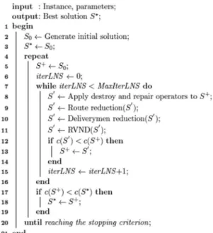
3.3 LNS-based metaheuristic approach
The second metaheuristic approach proposed in this paper is based on the LNS metaheuristic
(Shaw, 1998). LNS tries to overcome the dificulties
faced by many local search algorithms, which only generate little changes in the solutions. Therefore,
for these local searches it is often very dificult to
escape from local optimal solutions and explore promising areas of the solution space when dealing with tightly constrained problems. In LNS, a solution is gradually improved by alternately destroying and repairing it. A detailed description of LNS algorithms
is presented by Pisinger & Ropke (2010).
In the proposed approach, the LNS guides the search based on destroy and repair operators, in addition to the same improvement heuristics used in the ILS-based approach (RVND, route reduction heuristic and deliverymen reduction heuristic). The structure of the metaheuristic approach is shown in Figure 8. First, an initial solution is generated with the constructive heuristic (line 2). An outer
loop deines the initial solution as incumbent (line 5)
and apply the LNS operations until the stopping criteria is reached. In the main loop of the approach
(lines 7-16), the irst step is to apply the destroy
and repair operators (line 8), which are described in Sections 3.3.1 and 3.3.2. These operators are chosen at random from a set of available operators, which will be described below. Then, the route reduction, deliverymen reduction and RVND heuristics are applied
(lines 9-11). Only improved solutions are accepted
(lines 12-14) and the main loop inishes when the
algorithm reaches MaxIterLNS iterations. After that, the best global solution is updated (lines 17-19) and the outer loop is repeated in case that the overall
stopping criterion has not been satisied.
3.3.1 Destroy operators
The approach uses four different destroy operators.
Each one of them takes as input a complete solution
and returns a partial solution from which q clusters were removed. The used operators are:
• Random removal: this operator selects q
clusters at random and removes them from the
solution. As pointed out by Pisinger & Ropke
(2007), this operator clearly has the effect of diversifying the search.
• Worst removal: this operator tries to remove
clusters that are very expensive, or that somehow increase the cost of the current solution. Let i be a cluster, i– its predecessor and i+ its successor
in the route. The cost ci of cluster i is computed according to Equation 2.
, , ,
i i i i i i i
c =d− +d +−d− + (2)
where dij is the distance between clusters i and j. Next, the removal operator repeatedly chooses a new cluster i that has the largest cost, until q clusters have been removed. The removal operator has a randomization component, which is controlled by the parameter p as follows. Let L be the number of
clusters in the solution. When a new cluster must be removed, a random number y is chosen from the interval (0,1] and we calculate k y Lp
= . Next, the cluster with the kth largest cost is removed and L is updated. This procedure is repeated until q clusters are removed. Note that if p is large, more expensive
clusters are more likely to be selected, while less
expensive clusters may be chosen for smaller values of p. This component was incorporated to avoid situations where the same clusters are removed over
and over again, as in (Pisinger & Ropke, 2007).
• Related removal: the purpose of the related
removal operator is to remove clusters that are related in some sense and therefore it is expected that may be easy to interchange. The relatedness measure between two clusters i and j was computed as the distance between them, removing the
clusters as follows. The irst selected cluster
is chosen at random. Then, other clusters are selected, but they must be closely related to a previously selected cluster. This procedure is applied until q clusters are marked as selected. Then, these clusters are removed. Similar to the worst removal operator, the selection process contains a randomized component, which is controlled by the parameter p.
• Time-oriented removal: this operator is a
variant of the related removal operator. In this operator, the relatedness measure is based on the service start time on clusters. Hence, this operator tries to remove clusters that are served approximately at the same time, as it is expected that can may be easy interchangeable.
The operator works as follows. First, a cluster r
is chosen at random and its 2q closest clusters
are marked as potential clusters. The relatedness
measure between clusters r and i is given by Equation 3.
ri wr wi
∆ = − (3)
where wr and wi are the service start times at clusters
r and i, respectively. Among the potential clusters, the operator selects the q – 1 clusters that are the most related to r. These clusters are removed together with r. This operator also has a randomization component, similar to the worst removal and related removal operators.
3.3.2 Repair operators
After applying the destroy operator, the partial solution must be repaired in order to render it feasible
again. Each repair operator takes a partial solution
as input and returns a complete feasible solution. The used repair operators are described below.
• Greedy insertion: this operator tries to insert
the clusters in the cheapest possible position. Formally, it can be stated as follows. Let ∆fir
denote the change in the objective function incurred when inserting cluster i in the cheapest position in route r. If cluster i cannot be inserted in route r, then ∆ = ∞fir . Following a greedy
criterion, Equation 4 is applied.
( )
,, min ir
i r
i r′ ′ =arg ∆f (4)
and cluster i′ is inserted into the best position in route r′. This operation is performed until all clusters
have been reinserted into the solution or no more insertions are feasible. In the latter case, new routes are created (with the maximum possible crew) to serve those clusters.
• Regret insertion: this operator tries to overcome
the dificulties of the greedy insertion operator as it often postpones the insertion of dificult
clusters to the last iterations, when its insertion becomes more constrained. This operator tries to incorporate an anticipation component when selecting the next cluster to be inserted, as follows. Let q
i
f
∆ denote the change in the objective function when cluster i is inserted into its best position in the qth cheapest route. Then, in each call of the operator, we choose cluster i′ in accordance with Equation 5
2 1
max i i
i
i′=arg ∆ − ∆f f (5)
and the cluster is inserted into the route with the lowest insertion cost. In other words, the operator maximizes the difference of cost of inserting the cluster i in its second best route and its best route, meaning that groups with fewer feasible insertion
positions tend to be inserted irst. This process is
repeated until no more clusters can be inserted. As in the greedy insertion operator, if any cluster cannot be inserted new routes are created to visit those clusters.
4 Computational experiments
4.1 Benchmark instances
In all the experiments we use the benchmark
instances proposed by Pureza et al. (2012), which
are based on the well-known benchmark instances
proposed by Solomon (1987) for the VRP with time windows. The instance set is composed of 56 instances involving 100 clusters. They are divided into six classes based on planning horizon length, vehicle capacity, width of the time windows and distribution of the customers, namely: R1, R2, C1, C2, RC1 and RC2. Classes R1, C1 and RC1 (R2, C2 and RC2) contain instances with short (long) planning horizon, narrow (loose) time windows and vehicles with small (large) capacity. On the other hand, classes R1/R2, C1/C2 and RC1/RC2 have randomly distributed, grouped and a mix of randomly distributed and grouped clusters, respectively. Note that the characteristics of classes R2, C2 and RC2 allow more clusters to be served per route than in routes of classes R1, C1 and RC1.
In the original Solomon instances there is no differentiation of the service times according to the number of deliverymen. Thus, Pureza et al. (2012) proposed to modify them to represent the delivery time of the accumulated demand of the customers
on clusters, deined in Equation 6.
{
}
{
0 0}
min * , max ,
, 1, , , 1, 2, 3.
a
i i i i
il
rs q T w d d
s i n l
l
− −
= = … = (6)
where qi is the demand of cluster i, rs is the service
rate, which in our experiments was deined with
value 2, T is the latest arrival time at the depot and
0i i0
d =d is the distance between the depot and cluster
i, whereas the second term in the min operation in the equation guarantees the instance feasibility.
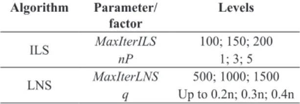
4.2 Parameter tuning
The metaheuristic approaches were calibrated using a Design of Experiments (Montgomery, 2012), as in Naderi et al. (2010). To do so, we carried out a full factorial experiment testing the parameters of the approaches in the levels shown in Table 2. The tested levels were determined through preliminary experiments. All levels combination resulted in nine
different conigurations for each algorithm. We used
20 instances (chosen at random from the instance set) to calibrate the algorithms. All 20 instances were solved
ive times by each coniguration of the algorithms,
resulting in 900 observations per approach. A time
limit of ive minutes was imposed for each single
execution of the algorithms, which were run on a PC Dell Precision T7600 CPU E5-6280 2.70 GHz and 192 GB of RAM, using a single core. To measure the performance, we used the relative gap between the cost of the solution found by the algorithm (Algsol)
and the cost of the best solution found by all the
conigurations (Minsol), as stated in Equation 7.
sol sol sol Alg Min gap Min −
= (7)
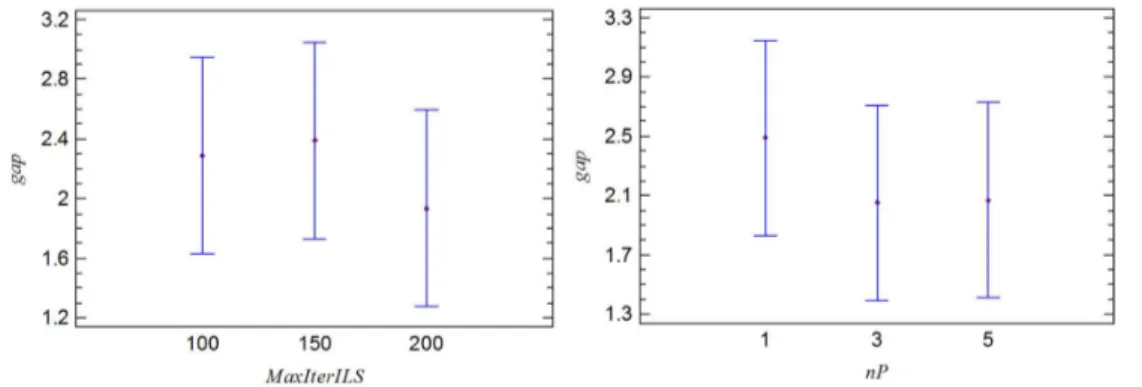
The results were analyzed using the analysis of
variance technique, checking the three hypotheses
of this analysis (normality, homoscedasticity and independence of residuals) using the appropriate techniques. No evidence was found to question the validity of the experiment. Figures 9-10 show the
mean plots and Tukey intervals with 95% conidence
for the levels of the parameters of the metaheuristic approaches. In these plots, overlapping between
conidence intervals indicates that there is no statistically signiicant difference between the means.
The plots in Figures 9 and 10 indicate that there
is no statistically signiicant difference between the
performances of the methods, considering all levels of the parameters. This result is explained by the fact that the metaheuristic approaches depend heavily on the additional heuristics (route reduction heuristic and deliverymen reduction heuristic), which have no parameters, thus they reduce the sensitivity of the metaheuristic approaches regarding to its parameters. The dependency of the approaches on the additional
heuristics is a result of the speciic characteristics of
the VRPTWMD.
Since there is no signiicant difference in the
performance of the approaches for different levels of
the parameters, values for them were deined based
on the best average results of the calibration tests, as follows: MaxIterILS = 200, nP = 3, MaxIterLNS = 1000 and q = rand(0,1 ; 0, 2n n). In addition, following the
proposal of Ropke & Pisinger (2006), the value of the
randomization component of the removal operators
in the LNS was deined as p=3. This value is large enough to allow removing clusters with large costs. Still, this value allows the removal operators to have an adequate performance, avoiding cases where the same clusters are removed repeatedly.
4.3 Experiments with the metaheuristic approaches
This section shows the results of the computational experiments after the tuning phase performed in the last section. For these experiments, the weights of the
Table 2. Factors and levels of the design of experiments.
Algorithm Parameter/ factor
Levels
ILS MaxIterILS 100; 150; 200
nP 1; 3; 5
objective function are deined with the same values
as used by Pureza et al. (2012), namely: p1=1, 0.1p2=
and p3=0.0001. They prioritize the minimization of
the number of vehicles used in the solution, followed by the number of deliverymen and then the traveled distance. The experiments were run in a PC Intel Core i7 3.40 GHz with 16 GB RAM, using a single core, with a time limit of 600 seconds and running
ive times each algorithm.
The results of the metaheuristic approaches are compared with the results reported by Pureza et al. (2012), regarding a Tabu Search approach (TS-PMR) and an Ant Colony Optimization algorithm (ACO-PMR), which were both run in a PC Intel Core2 2.40 GHz with 2 GB RAM. Also, we use the results reported by Senarclens de Grancy & Reimann (2014), which were obtained by an ACO algorithm (ACO-SR), in a PC Intel E8400. In the following tables, labels Cost, Veh, Dist, Del and Time denote the total cost of the solutions, the number of vehicles used, the distance traveled, the number of deliverymen assigned and the running time (in seconds), respectively. The best results (in terms of cost) for each instance/class are highlighted in boldface. Costs are presented with two
decimal places only and ties are broken by selecting
the solution with the shortest distance.
First, we compare the overall performance of the approaches in all the instance classes. In this sense, it is only possible to compare our approaches with the approaches of Pureza et al. (2012), since Senarclens de Grancy & Reimann (2014) only report the results for class R1. Table 3 shows the best results obtained by the metaheuristic approaches, grouped for each instance class. Note that the proposed approaches
always ind solutions with costs that are better than
or equal to those found by TS-PMR and ACO-PMR in all instance classes. Moreover, comparing in detail the performance of the two proposed approaches,
we obtain that ILS inds the best solution in 9 out of
12 instances in class R1, in 5 out of 8 in class RC1, in 9 out of 11 of class R2 and in 4 out of 8 of class
RC2. In classes C1 and C2, both approaches ind
the same solutions for each instance. As a result, ILS is superior to LNS regarding the number of best solutions found. On the other hand, in terms of average results ILS is better than LNS only in one instance class, whereas LNS is superior in three classes and tie in the two remaining classes. This result indicates that when LNS surpass ILS in a single instance, the difference is large enough to allow dominating in terms of average results.
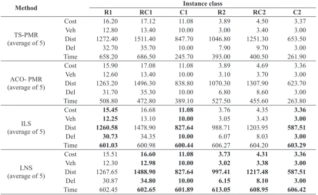
Table 4 presents the average results (grouped for
each instance class), considering the ive runs of Figure 9. Means plots and Tukey intervals for the parameters of the ILS.
routes in these instances are in general shorter. This class was also addressed in detail in previous researches related to the VRPTWMD. Table 5 shows the best solutions found by the ILS and LNS metaheuristic approaches, as well as the best solutions reported by Pureza et al. (2012) and Senarclens de Grancy each instance. Similar to results of Table 3, it can
be seen that the ILS and LNS approaches dominated ACO-PMR and TS-PMR in all instance classes.
The results obtained for the instance class R1 are now described in detail, as their characteristics better
relect the importance of the service times, since the
Table 3. Best results (grouped) of the metaheuristic approaches.
Method Instance class
R1 RC1 C1 R2 RC2 C2
TS-PMR (best out of 5)
Cost 15.70 16.64 11.08 3.75 4.45 3.36
Veh 12.33 13.00 10.00 2.90 3.40 3.00
Dist 1258.00 1527.90 830.70 1034.00 1230.40 597.20
Del 32.42 34.90 10.00 7.50 9.30 3.00
Time 640.10 677.10 265.10 425.40 419.10 246.80
ACO- PMR (best out of 5)
Cost 15.77 16.70 11.08 3.86 4.58 3.36
Veh 12.50 13.00 10.00 3.10 3.60 3.00
Dist 1261.50 1480.10 833.60 1064.20 1296.00 609.30
Del 31.40 35.50 10.00 6.50 8.50 3.00
Time 575.80 508.60 375.20 600.60 462.00 243.30
ILS (best out of 5)
Cost 15.34 16.59 11.08 3.63 4.31 3.36
Veh 12.17 13.00 10.00 2.91 3.38 3.00
Dist 1271.71 1482.46 827.64 993.17 1186.61 587.51
Del 30.50 34.38 10.00 6.18 8.13 3.00
Time 600.75 601.25 600.22 604.09 603.25 601.50
LNS (best out of 5)
Cost 15.32 16.50 11.08 3.64 4.29 3.36
Veh 12.08 12.88 10.00 2.91 3.38 3.00
Dist 1271.64 1492.29 827.64 998.00 1197.49 587.51
Del 31.08 34.75 10.00 6.27 8.00 3.00
Time 602.42 603.25 600.67 610.09 609.50 602.75
Table 4. Average results (grouped) of the metaheuristic approaches.
Method Instance class
R1 RC1 C1 R2 RC2 C2
TS-PMR (average of 5)
Cost 16.20 17.12 11.08 3.89 4.50 3.37
Veh 12.80 13.40 10.00 3.00 3.40 3.00
Dist 1272.40 1511.40 847.70 1046.80 1251.30 653.50
Del 32.70 35.70 10.00 7.90 9.70 3.00
Time 658.20 686.50 245.70 393.00 400.50 261.90
ACO- PMR (average of 5)
Cost 15.90 17.08 11.08 3.89 4.69 3.36
Veh 12.60 13.40 10.00 3.10 3.70 3.00
Dist 1263.20 1496.30 838.80 1070.30 1307.90 623.70
Del 31.70 35.30 10.00 6.80 8.60 3.00
Time 508.80 472.80 389.10 527.50 455.60 263.80
ILS (average of 5)
Cost 15.45 16.68 11.08 3.76 4.35 3.36
Veh 12.25 13.10 10.00 3.05 3.43 3.00
Dist 1260.58 1478.90 827.64 988.71 1203.95 587.51
Del 30.73 34.35 10.00 6.07 8.03 3.00
Time 601.03 600.98 600.44 606.27 604.20 603.29
LNS (average of 5)
Cost 15.51 16.60 11.08 3.73 4.31 3.36
Veh 12.30 12.98 10.00 3.02 3.38 3.00
Dist 1267.65 1488.90 827.64 997.41 1217.48 587.51
Del 30.87 34.80 10.00 6.15 8.10 3.00
Álvar
ez, A. et al.
Gest. Pr
od.
, São Carlos, v
. 23, n. 2, p. 279-293, 2016
Method Instance Avg Sum
R101 R102 R103 R104 R105 R106 R107 R108 R109 R110 R111 R112
TS-PMR (best out of 5)
Cost 23.67 21.05 16.33 12.91 17.84 15.23 13.01 12.80 15.43 14.12 13.11 12.90 15.70 188.41
Veh 19 17 13 10 14 12 10 10 12 11 10 10 12.33 148
Dist 1740.00 1520.00 1285.00 1057.00 1446.00 1323.00 1112.00 967.00 1296.00 1217.00 1137.00 996.00 1258.00 15096.00
Del 45 39 32 28 37 31 29 27 33 30 30 28 32.42 389
Time 645 655 959 692 463 492 473 953 428 620 616 686 640.17 7682
ACO-SR (best out of 5)
Cost 23.67 20.95 15.94 12.70 17.64 15.13 12.81 11.70 15.12 13.92 13.01 11.80 15.37 184.40
Veh 19 17 13 10 14 12 10 9 12 11 10 9 12.17 146
Dist 1725.46 1533.40 1371.63 1045.68 1412.52 1301.34 1108.92 967.18 1229.72 1154.95 1134.16 996.32 1248.44 14981.28
Del 45 38 28 26 35 30 27 26 30 28 29 27 30.75 369
Time 960 960 960 960 960 960 960 960 960 960 960 960 960.00 11520
ILS (best out of 5)
Cost 23.68 20.95 15.84 12.71 17.64 15.04 12.81 11.70 15.03 13.92 13.02 11.80 15.34 184.13
Veh 19 17 13 10 14 12 10 9 12 11 10 9 12.17 146
Dist 1757.40 1530.92 1410.73 1062.58 1412.52 1352.09 1140.79 965.31 1291.62 1187.49 1161.96 987.14 1271.71 15260.57
Del 45 38 27 26 35 29 27 26 29 28 29 27 30.50 366
Time 600 601 601 601 600 600 603 601 600 600 602 600 600.75 7209
LNS (best out of 5)
Cost 23.68 20.95 15.94 12.71 17.64 15.03 12.91 11.70 14.43 13.92 13.11 11.80 15.32 183.83
Veh 19 17 13 10 14 12 10 9 11 11 10 9 12.08 145
Dist 1755.04 1531.36 1369.12 1072.41 1412.52 1328.21 1139.96 1011.37 1281.84 1219.12 1149.03 989.70 1271.64 15259.70
Del 45 38 28 26 35 29 28 26 33 28 30 27 31.08 373
oaches for the vehicle r
outing pr
oblem...
291
Instance Average results (standard deviation) ILS Average results (standard deviation) LNS
Cost Veh Dist Del Time Cost Veh Dist Del Time
R101 23.75(0.04) 19.00(0.00) 1737.37(11.99) 45.80(0.45) 600.20(0.45) 23.73(0.05) 19.00(0.00) 1739.67(14.54) 45.60(0.55) 600.60(0.89)
R102 20.95(0.00) 17.00(0.00) 1531.27(0.19) 38.00(0.00) 600.80(0.84) 20.95(0.00) 17.00(0.00) 1531.66(0.34) 38.00(0.00) 601.40(1.14)
R103 15.94(0.07) 13.00(0.00) 1375.83(23.83) 28.00(0.71) 601.60(1.95) 15.94(0.00) 13.00(0.00) 1380.77(13.08) 28.00(0.00) 602.60(1.14)
R104 12.73(0.04) 10.00(0.00) 1063.26(13.97) 26.20(0.45) 602.20(1.30) 12.79(0.04) 10.00(0.00) 1061.47(6.51) 26.80(0.45) 605.60(2.51)
R105 17.64(0.00) 14.00(0.00) 1412.52(0.00) 35.00(0.00) 600.00 (0.00) 17.64(0.00) 14.00(0.00) 1413.21(1.02) 35.00(0.00) 600.40(0.55)
R106 15.11(0.04) 12.00(0.00) 1307.63(25.17) 29.80(0.45) 601.40(1.14) 15.07(0.05) 12.00(0.00) 1334.82(43.79) 29.40(0.55) 600.40(0.55)
R107 12.95(0.11) 10.00(0.00) 1127.93(15.21) 28.40(1.14) 601.20(1.10) 12.97(0.05) 10.00(0.00) 1137.38(21.06) 28.60(0.55) 600.80(1.79)
R108 11.72(0.04) 9.00(0.00) 975.94(9.06) 26.20(0.45) 601.40(0.89) 11.94(0.37) 9.20(0.45) 989.26(16.40) 26.40(0.89) 602.60(2.07)
R109 15.09(0.05) 12.00(0.00) 1261.06(35.47) 29.60(0.55) 600.40(0.55) 14.99(0.31) 11.80(0.45) 1278.42(6.91) 30.60(1.34) 602.80(1.48)
R110 13.94(0.04) 11.00(0.00) 1184.00(26.59) 28.20(0.45) 601.00 (1.00) 13.96(0.05) 11.00(0.00) 1203.71(34.82) 28.40(0.55) 602.40(2.30)
R111 13.61(0.34) 10.80(0.45) 1138.48(25.28) 27.00 (1.22) 601.40(1.34) 13.65(0.30) 10.80(0.45) 1135.86(9.86) 27.40(1.52) 604.40(2.70)
Acknowledgements
This research was supported by CAPES-DS, FAPESP under project number 2014/00939-8 and CNPq under project number 482664/2013-4.
References
Azi, N., Gendreau, M., & Potvin, J. Y. (2014). An adaptive large neighborhood search for a vehicle routing problem with multiple routes. Computers & Operations Research, 41(1), 167-173. http://dx.doi.org/10.1016/j. cor.2013.08.016.
Bräysy, O., & Gendreau, M. (2005). Vehicle Routing Problem with Time Windows, Part I: Route Construction and Local Search Algorithms. Transportation Science, 39(1), 104-118. http://dx.doi.org/10.1287/trsc.1030.0056.
Ferreira, V., & Pureza, V. (2012). Some experiments with a savings heuristic and a tabu search approach for the vehicle routing problem with multiple deliverymen. Pesquisa Operacional, 32(2), 443-463. http://dx.doi. org/10.1590/S0101-74382012005000016.
Hong, L. (2012). An improved LNS algorithm for real-time vehicle routing problem with time windows. Computers & Operations Research, 39(2), 151-163. http://dx.doi. org/10.1016/j.cor.2011.03.006.
Lourenço, H., Martin, O., & Stützle, T. (2010). Iterated local search: framework and applications. In M. Gendreau & J.-Y. Potvin (Eds.), Handbook of metaheuristics (pp. 363-397). Boston, MA: Springer US.
Lourenço, H. R., Martin, O. C., & Stutzle, T. (2003). Iterated local search. In F. Glover & G. A. Kochenberger (Eds.), Handbook of metaheuristics (pp. 321-353). Boston: Springer US.
Melechovsky, J. (2012). Evolutionary local search algorithm to solve the multi-compartment vehicle routing problem with time windows. In Proceedings of the XXX International Conference Mathematical Methods in Economics (pp. 564-568). Karviná: Silesian University.
Mladenovic, N., & Hansen, P. (1997). Variable neighborhood search. Computers & Operations Research, 24(11), 1097-1100. http://dx.doi.org/10.1016/S0305-0548(97)00031-2.
Montgomery, D. C. (2012). Design and analysis of experiments (Vol. 2). Hoboken: Wiley.
Naderi, B., Ruiz, R., & Zandieh, M. (2010). Algorithms for a realistic variant of flowshop scheduling. Computers & Operations Research, 37(2), 236-246. http://dx.doi. org/10.1016/j.cor.2009.04.017.
Pisinger, D., & Ropke, S. (2007). A general heuristic for vehicle routing problems. Computers & Operations Research, 34(8), 2403-2435. http://dx.doi.org/10.1016/j. cor.2005.09.012.
Pisinger, D., & Ropke, S. (2010). Large neighborhood search. In M. Gendreau & J.-Y. Potvin. Handbook of metaheuristics (Vol. 146, pp. 1-22). Boston: Springer US.
& Reimann (2014). In the latter, two metaheuristic algorithms were proposed, namely, ACO and GRASP algorithms. We compare only with ACO, as it had the best performance in class R1. The results show that
ILS and LNS can ind the best solution in 6 out of
12 instances of the class. Comparing with TS-PMR,
ILS inds solutions using 1.35% and 5.91% less
vehicles and deliverymen respectively, whereas
LNS inds solutions using 2.03% and 4.11% less
vehicles and deliverymen respectively. On the other
hand, comparing with ACO-SR, ILS inds solutions
using the same number of vehicles and 0.81% less
deliverymen, while LNS inds solutions using 0.68%
less vehicles and 1.08% more deliverymen. Recall that for instance R101, whose optimal solution is
known, ILS and LNS ind solutions with the optimal
number of vehicles and deliverymen, while with travel distances 2.17% and 2.03% longer than in the optimal solution, respectively.
Finally, to show the robustness of the proposed approaches and, considering that both algorithm have randomized components, Table 6 presents the average values and standard deviations (in parentheses) of the cost of the solutions, the numbers of vehicles, the distances, the number of deliverymen and the
running times (in seconds), considering the ive runs
of the algorithms for instance class R1. Note that the standard deviations are relatively small when compared to the average values.
5 Conclusions and perspectives
In this paper, we have addressed the vehicle routing problem with time windows and multiple deliverymen using two metaheuristic approaches, which are based on Iterated Local Search and Large Neighborhood Search. Both approaches use the same constructive heuristic and also a set of additional heuristics, used to enhance the performance of the approaches. The additional
heuristics were developed to address speciic features
of the VRPTWMD. Using six instance classes from the literature, we have compared the performance of the approaches between themselves and against existing metaheuristics. Computational experiments showed that the developed metaheuristic approaches do not dominate one another in all the instance classes, and that both are capable of producing good solutions for the instances when compared to the other approaches from the literature. Perspectives for future research include the combination of these approaches with exact methods, such as column generation or general-purpose integer programming solvers, in order to derive hybrid methods for the VRPTWMD. Also, the current problem can also be extended to
incorporate practical features as heterogeneous leet,
Silva, M. M., Subramanian, A., & Ochi, L. S. (2015). An iterated local search heuristic for the split delivery vehicle routing problem. Computers & Operations Research, 53, 234-249. http://dx.doi.org/10.1016/j. cor.2014.08.005.
Solomon, M. (1987). Algorithms for the vehicle routing and scheduling problems with time window constraints. Operations Research, 35(2), 254-265. http://dx.doi. org/10.1287/opre.35.2.254.
Subramanian, A., Penna, P. H. V., Uchoa, E., & Ochi, L. S. (2012). A hybrid algorithm for the Heterogeneous Fleet Vehicle Routing Problem. European Journal of Operational Research, 221(2), 285-295. http://dx.doi. org/10.1016/j.ejor.2012.03.016.
Toth, P., & Vigo, D. (2002). The vehicle routing problem: the vehicle routing problem. Canada: Society for Industrial and Applied Mathematics. http://dx.doi. org/10.1137/1.9780898718515.
Pureza, V., Morabito, R., & Reimann, M. (2012). Vehicle routing with multiple deliverymen: Modeling and heuristic approaches for the VRPTW. European Journal of Operational Research, 218(3), 636-647. http://dx.doi. org/10.1016/j.ejor.2011.12.005.
Ropke, S., & Pisinger, D. (2006). An adaptive large neighborhood search heuristic for the pickup and delivery problem with time windows. Transportation Science, 40(4), 455-472. http://dx.doi.org/10.1287/ trsc.1050.0135.
Senarclens de Grancy, G., & Reimann, M. (2014). Vehicle routing problems with time windows and multiple service workers: a systematic comparison between ACO and GRASP. Central European Journal of Operations Research, 24(1): 29-48.