Statistical Fatigue Experiment Design in Medium Density
Fiberboard
Mariano Martínez Espinosa
a, Carlito Calil Jr.
baInstituto de Física de São Carlos, Universidade de São Paulo, São Carlos – SP, Brazil bEscola de Engenharia de São Carlos, Universidade de São Paulo,
São Carlos – SP, Brazil
Received: March 21, 2000; Revised: July 31, 2000
Medium Density Fiberboard (MDF) is a wood-based composite widely employed in several industrial applications, in addition to its use in structures subjected to dynamic loads. Its fatigue-re-lated aspects, however, have been consistently ignored. This work proposes to study fatigue in MDF, including the following factors: the basic concepts of MDF and fatigue and the statistical design of fatigue experiments in MDF, with the purpose of obtaining accurate information for analysis by means of statistical methods. The results of our tests revealed that the statistical model is suitable to fit the number of cycles in intermediary S and f levels and to determine the levels of the factors that maximize the total number of cycles to failure. It was also found that the proposed design is of great practical interest for fatigue strength in the tension in wood and wood derivatives.
Keywords:MDF, fatigue, fatigue properties in wood composites, factorial designs
1. Introduction
The properties of wood composites, as well as cost and manufacturing considerations, suggest that these are the most suitable materials for several industrial applications such as furniture, civil construction and other uses. These products, called composites, are materials composed of combinations of various elements, mainly wood particles and glue, having different properties of solid wood1.
One wood-based composite that is widely used in a variety of industrial applications is Medium Density Fiber-board (MDF)9. However, the aspects related to fatigue in this product have generally been ignored11, although most service failures associated to mechanical causes of the materials are usually fatigue-related7.
Fatigue studies of MDF are possible due to its general properties and characteristics8. However, for such pur-poses, an appropriate statistical experiment design must be made to obtain accurate information for analysis by means of statistical methods in order to reach valid and objective inferences6.
The use of statistical experiment design in the study of the fatigue in MDF in particular is justified by several factors such as the reduced number of tests, reduced testing time and, thus, reduced cost, less variability and greater reliability of the results, among others. However, the main
reason is to obtain appropriate data that is analyzable using the appropriate methods and statistical techniques, since the analysis method and technique depend directly on the design used15.
Therefore, the objective of this work is to carry out an experiment plan for the study of the fatigue strength in the tension in MDF in order to reduce the cost, time and variability of the results. Another objective is to envision a possible appropriate statistical model for MDF fatigue data using the experimental results of the proposed tests.
2. Medium Density Fiberboard (MDF)
Medium Density Fiberboard (MDF) is the generic name used to define a sheet composed mainly of lignin-cellulosic fibers combined with a synthetic resin or some other suit-able adhesive system, glued together by means of pressure and heat. The introduction of additives during the manu-facturing process can improve the dimensional stability, fire resistance and impermeability of MDF17.
MDF is a homogeneous, uniform and stable product with a flat surface having good workability, machinability and wide acceptance for coatings with several finishes. It is widely employed by the furniture industry owing to its sturdiness and uniformity, which ensure satisfactory results with conventional techniques (screwing, rabeting, cutting
a
e-mail: [email protected] b
to size, gluing, etc.) and its characteristics of mechanical strength allow for its use even in structural panels9.
MDF can also be used advantageously in the production of lathe-turned and milled pieces which, until recently, had been made of solid wood, such as curtain rods, parts for chairs etc19.
3. MDF Fatigue
Fatigue is a structural failure caused by a material being subjected to repeated stress or cyclic loading for a consid-erable period of service time.
The stresses a material can bear under cyclic loading are much smaller than those bearable under static loading. In other words, a fatigue-related failure may occur at a much lesser stress than the limit of the material’s strength. Three basic factors generally cause fatigue-related fail-ure10:
1) high maximum tensile stress;
2) great variation or fluctuation of applied stress; 3) a large number of stress application cycles.
A cycle is an interval of time during which a sequence of stresses is cyclically applied to the specimen in the same regular order. Stress is the quotient of intensity of a force by the specimen’s surface area.
The stress waves used in fatigue tests are generally triangular, square or sinusoidal and the typical cycles of stress in fatigue are reverse stresses, fluctuating stress and irregular or random stress10.
The properties of fatigue in wood and wooden products (e.g., laminated wood) are particularly influenced by the following factors11:
1) The wood species, place of origin, density, etc. 2) The size and shape of the test specimen. 3) The moisture content.
4) The type of applied load. Experiments normally consist of tension, compression, bending or shear tests or a combination of these. Most fatigue experiments are made with harmonic loads and there are three important factors in this type of load:
• The R-ratio (the ration between the minimum and maximum tension).
• The value of the stress.
• The frequency (loading time), which must be taken in account.
5) Other factors affecting the properties of fatigue in wood are temperature, chemical treatments, adhesives, glu-ing, etc.
Although MDF has no specific properties of fatigue, its properties and general characteristics facilitate the study of fatigue of this material. Thus, since MDF is a homogeneous and approximately isotropic material, the stages of rupture of an isotropic material subject to fatigue can be considered for its study.
4. Statistical Experiment Design
Statistical experiment design is the process of designing an experiment to obtain appropriate data that can be ana-lyzed using statistical methods in order to reach valid and objective conclusions.
Experiment design is essential in engineering to im-prove the performance of a manufacturing process. Experi-ment design is also widely employed in the developExperi-ment of new processes. The application of experiment design techniques during the initial phase of process development can lead to improved process performance, less variability, shorter development time and, thus, reduced overall cost.
The application of experiment design is simple, al-though certain requisites must be followed. The two main requirements in experiment design are to obtain aleatory and replicable results15.
4.1. Selection of the variable responses, factors and levels in experiment design
When selecting the dependent response or variable, the experimentor must be certain that the response that will be measured actually provides useful information about the process under study. In experiment design, the average of the measured characteristic is usually the response vari-able; therefore, replicates should be made6.
In experiment design, a factor (independent variable) is a qualitative or quantitative experimental variable, which is investigated to determine its effect on a response. The specific values of factors are called levels and can be determined a priori13. From a statistical standpoint, it is recommended that two or, at the most, three levels be used per factor since, if the number of levels increases, the number of tests will greatly increase.
4.2. Factorial design
In many experimental engineering situations one knows in advance that some factors produce different re-sponses. One particular case of this is the study of material fatigue. When a response is influenced by certain factors, it can be shown that, in general, factorial design is the most efficient. Factorial design is the type of design in which all the possible combinations of factorial levels are investi-gated in each test15.
A complete factorial design with k factors (variables) is obtained by choosing n1levels of factor 1, n2levels of
factor 2, , nklevels of factor k, and then selecting the n = n1
x n2 x x nk experiments obtained, using every possible
4.2.1 Desirable properties of factorial designs15:
• They should direct the investigation, since they are particularly useful in the exploratory stage of research.
• They should indicate the size of the sample to be selected.
• They should allow for multiple comparisons, thus facilitating the creation and critique of models.
•They should provide highly efficient parameter esti-mators.
However, the most significant argument set forth is that they should allow for models to be seen in the data in the specification stage of the model (in the specification of a functional relationship).
4.2.2. Approximate response functions
Engineering, physics, chemistry, biology and other fields of research are often interested in a functional rela-tionship. Such a relationship can be obtained through fac-torial designing using the following approximations6:
E(y) = η =f(x∗ 1, x
∗ 2, ..., x
∗ k) =f(X
~∗) (1)
which relates the expectedηvalue of a y response, such as a number of cycles (or production percentage, purity, viscosity, etc.) to k quantitative or qualitative variables x1*, x2*, , xk*, such as stress, frequency, temperature, time,
pressure, concentration, etc.
Thef(X~∗)function can assume a great variety of forms: linear, parabolic, exponential, etc. These forms are impor-tant because they approximate many real world relation-ships, in addition to being relatively easy to work with and interpret5,6. However, because reiterated tests are made for the sameX~∗conditions, the measurements of the y response would vary because of measurement and observational errors and the basic variability of the experimental mate-rial5.
The variations of y, in practice, are the differences between the observed y values and the expectedηvalues. These differences, generally indicated byε(epsilon, fifth letter of the Greek alphabet), are called residues and are aleatory variables with some degree of distribution of prob-ability around their meanηvalue6. Therefore, our general objective is to investigate certain aspects of a functional relationship affected by an error and expressed as5:
y=f(X~∗) + ε (2)
In many practical problems, however, the form of the real relationship between the dependent (y) variable and the independent (X~∗) variables is unknown. Hence, an appro-priate approximation of the real (y) function and the set of independent variables must be determined, normally using first and second order polynomials. The latter is the most frequently used, since it allows a curve of the response to be analyzed, which facilitates modeling the relationship
between the response and each factor using a linear or quadratic function.
Second order models should involve at least three levels of each factor to allow for an estimate of the model’s coefficients. There are many factorial designs that could be used to estimate a second order model. In this study, be-cause only the effect of two independent variables was verified, we will use a three-level factorial design (3k).
4.2.3. Three-level factorial designs (3k)
Three-level factorial designs are formed by k factors, each one having three levels. In a 3k design or in any factorial design it is more practical not to have to deal with the actual numerical measurements of the xi* variables,
working, instead, with coded xicvariables, i.e., coding the
levels of the factors. Codification is done mainly for the following reasons14:
1) If the independent variables are qualitative, they are not numeric; thus, their values need to be coded to estimate a regression model.
2) Although the independent quantitative variables are numeric, they should also be coded to estimate a regression model, for the following reasons:
2.1) To estimate the parameters of the model, a matrix termed (X’*, X*) should be inverted. Considerable round-ing out errors may occur durround-ing the inversion process if the absolute values of the numbers in the (X’*, X*) matrix vary significantly, which usually leads to errors in the estimates of parameters. Coding facilitates the computational inver-sion of the matrix, reducing calculation errors and allowing for more accurate parameter estimates.
2.2) A second reason for coding quantitative variables is the problem of multicolinearity, which is the existence of an exact or approximately exact linear relationship among the independent variables. The problem of multi-colinearity is inevitable in estimates of regression models (e.g., second-order models), particularly when higher-or-der terms are estimated. In quadratic models, for instance, in which the two x1* and x12* variables are normally highly
correlated, the probability of rounding out errors in the coefficients of regression increases in the presence of mul-ticolinearity. These problems are usually eliminated with coding.
The coding of the levels of the factors of the most frequently used 3kdesign is -1, 0 and 1, which denote the factor’s low, intermediate and high levels, respectively, as illustrated in Table 1. This code is obtained theoretically by the following equation5:
xci=
x∗ i−x
x
_
∗ i=
x∗
−1+x ∗ 0+x
∗ 1
3 ,
S∗ i=x
∗ 0−x
∗ −1
or
S∗ i=x
∗ 1−x
∗ 0,
where x-1*, x0* and x1* are the values corresponding to the low, intermediate and high levels, respectively. Thus, (4) is used instead of (1), where (4) is given by:
E(y)= η=f(x1c, xc 2, ..., x
c k) =f(X
~c
) + ε (4)
A particularly important aspect in this study is the design, i.e., two factors each having three levels; our inter-est in this design lies in determining if the number of cycles to failure depends on stress and frequency factors.
a) Determining the effects of a 32design
The effect of the factors on the response is measured by the change in the average response in two or more combi-nations of the levels. In this type of factorial design there are 9 combinations of treatments. Thus, there are eight degrees of freedom between these combinations. The main A and B effects each have two degrees of freedom, while the AB interaction has four degrees of freedom. If there are (p*) replicates, there is a total of p* 32 - 1 degrees of freedom, which corresponds to 32 (p* - 1) degrees of freedom for the error15.
The combinations of treatments are written in standard order, which means that one factor at a time is introduced successively, combining each level with the set of the factors’ levels. The standard order for a 32design is 00, 10, 20, 01, 11, 21, 02, 12, 2215.
YATES’ algorithm (YATES’ modified algorithm gen-eralized for the 3kseries) can be used to calculate the effects and the respective square sum of a 32design. The use of this algorithm is simple and consists of determining some columns of data. A simplified calculation procedure is given below for the specific case of k = 2:
1) Calculate the total response of each (i) test, i.e., the total of each replicate. This column will be denoted be Y*. 2) Using the Y* column, calculate the Y*1column. The
Y*1values are calculated as follows: The first third of the column consists of the sum of each of the three sets of the three values of column Y*, i.e., y1* + y2* + y3*; y4* + y5* + y6* and y7* + y8* + y9*. The second third is the third observation minus the first one of each of the three previous sets, i.e., y3* - y1*; y6* - y4* and y9* - y7*. The last third of column Y*1is the result of the sum of the first and third observations, minus twice the second one, in each set of three observations, i.e., y1* - 2y2* + y3*; y4* - 2y5* + y6* and y7* - 2y8* + y9*.
3) Calculate the column denoted by Y*2. The values of this column are calculated by the same procedure as that used to determine the Y*1values, using the elements of the
Y*1column.
4) Calculate the elements of the divisor column D* using the expression 2r3tp*, where r is the number of factors
in the effect considered, t is the number of factors in the experiment minus the number of linear terms (levels 1) in this effect, and p* is the number of replicates.
1) Calculate the column of effects of the E* factors, which is obtained by dividing column Y*2by column D*.
2) Calculate the sums of squares (SQ), which is done by squaring the elements of column Y*2and dividing the result by the corresponding element of the divisor column. The sum of squares column now contains all the informa-tion required to construct the table of variance analyses. However, before the table of variance analyses is built, one must check if the data residuals have a constant variance and normal distribution.
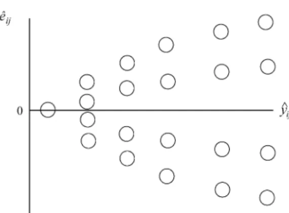
One of the tools most commonly used to confirm if the variance is constant consists of plotting the residuals (êij) vs. the estimated values (y^ij). This graph should not reveal any obvious pattern. One of the problems that is occasion-ally observed in such graphs is nonconstant variance, in which the residuals graph compared against the estimated values presents a funnel form; see Fig. 1. Variable variance also generally occurs in cases where the data does not follow a normal distribution. The assumption of normality can be confirmed by plotting a histogram of the residuals, which should have a symmetrical form. For this kind of verification, a normal probability graph (NSCORES) can also be used with the residuals, in which the residuals vs. the normal n-scores are represented. If the graph presents an approximately straight line, the distribution is approxi-mately normal. If the variance is nonconstant and if the Table 1.Notations used in a factorial design 32, withp* replicates.
Run (i) Response (Y) Factors
A B
1 y11... y1p* -1 -1
2 y21... y2p* 0 -1
3 y31... y3p* 1 -1
4 y41... y4p* -1 0
5 y51... y5p* 0 0
6 y61... y6p* 1 0
7 y71... y7p* -1 1
8 y81... y8p* 0 1
9 y91... y9p* 1 1
Note:y11, ... ,y9pin the table 1 they indicate the replicates of the response
assumption of normality is not followed, then the original data have to be transformed.
A logarithmic transformation is usually considered in fatigue data to stabilize their variance and lead to their normal distribution3.
The êijresiduals for the factorial 32design are calculated
by the following equation6:
e^ij=yij−y^ij (5)
Withy^ij=y
_
ij, wherey _
ijare the averages of the
observa-tions in the ith test. Therefore, (5) can also be expressed as:
e^ij=yij−y
_
ij (6)
5. Materials and Methods
This section discusses the aspects relating to the mate-rials used in the development of the work, directed at obtaining the values of fatigue strength in MDF, consider-ing the statistical factors in mechanical tests12.
•Material used in this study:MDF in sheets, supplied by a sawmill in the city of São Carlos, with dimensions of 1,83 m width, 2,75 m length and 15 mm thickness.
• Sampling Method: The specimens were removed from the fiberboard by the simple aleatory method, with 18 specimens selected at random according to the experiment designs indicated in the previous section and based on the ASTM: D1037/96a2code.
•Dimensioning and preparation of the specimens:
To determine the tensile fatigue strength in MDF, the specimens used followed the dimensions established by the ASTM: D1037/96a2code, as shown in Fig. 2. The T value indicates the thickness of the specimen, which should not exceed 254 mm.
•Execution of the tests:The static and dynamic tests were carried out in the DARTEC M1000/RC universal testing machine at LaMEM. The data obtained from the static tests were used to establish the levels of maximum and minimum tension for the fatigue tests. The static tests followed the recommendations of the ASTM: D1037/96a2 code and the NBR/7190/9716 code. Reverse stress cycles
of sinusoidal form were used in the dynamic tests, consid-ering frequencies of 1; 5 and 9 Hz for the specimens and cyclic loads of 60, 75 and 90 percent of the material’s strength, estimated in the static tests (on average Fr= 9.94 kN in dry condition). The procedure and results of the static tests employed are part of the work of MARTÍNEZ and CALIL on static tensile strength tests parallel to the surface in MDF12.
•Design:A factorial 32design was used, in which a study is made of the total number of cycles to failure per Y second (response variable), considering two replicates and using combinations of two factors (stress and frequency), each tested with three levels. The levels for each factor, as well as the coding for each level, are given in Table 2, in which the -1, 0 and 1 codes are obtained by Eq. (3), as follows:
x1c=
x∗ 1−75
15 , x
c 2=
x∗ 2−5
4
where, Figure 1.Plot of residualsvs. fitted values (no constant variance).
Figure 2.Dimensions of the specimens for tension test parallel to surface (mm).
Table 2.Number of cycles, under three levels of stress and three types of frequencies.
Coded levels xic -1 0 1
Stress (S) in % x1* 60 75 90
f∗ 10=
60+75+90
3 =75, f
∗ 20=
1+5+9
3 =5, and, S1 *= 75
– 60 = 15 and S2* = 5 – 1 = 4.
6. Results
Table 3 presents the experimental results, considering the notation given in Table 2.
7. Data Analyses
In agreement with section 4.2.3 (a), the analysis of the data begins with the graph of the residuals vs. the estimated values (Figs. 3 and 4).
Figure 3 indicates that the variance is nonconstant, i.e., it increases. When this is the case, a logarithmic transfor-mation of the data (YT= log (y)) is usually carried out to stabilize the variance.
An analysis of Fig. 4 indicates that the residues are not distributed, since a comparison of the residue graph against the normal scores does not follow a straight line. Proceed-ing with the transformed data construct, the residuals vs. estimated values are plotted (Fig. 5). Figure 5 indicates a constant variance, while the behavior shown in Fig. 6 is approximately linear, indicating that the residuals follow
an almost normal distribution. Hence, the YATES algo-rithm is used in the transformed data to determine the effects of the factors.
Table 4 shows that the greatest effects for the number of cycles, in decreasing order, are stress (SL= -0.97017), frequency (fL = 0.33887) and stress to the square (SQ= -0.09234). However, the quadratic effect of S is not as significant as the individual effects of f and S (main effects of f and S), respectively.
Table 3.Data of MDF obtained in the factorial design 32.
Run (i) Response (Y) Factors
yi1 yi2 S F
1 6201 9423 -1 -1
2 1831 1447 0 -1
3 91 108 1 -1
4 17158 22885 -1 0
5 4405 5362 0 0
6 214 153 1 0
7 43051 37736 -1 1
8 6263 6597 0 1
9 548 482 1 1
Figure 4.Plot of residualsvs. the normal scores.
Figure 3.Plot of residualsvs. fitted values.
Figure 5.Plot of residualsvs. the fitted values (transformed data).
culate the normal scores of the effects and plot the effects
vs. the normal scores (Fig. 7). All the effects that are located
approximately under the straight line are insignificant, while the significant effects are far removed from it. The effects that are identified in this analysis are the main effects of f and S, and no significant interaction is observed among the factors considered.
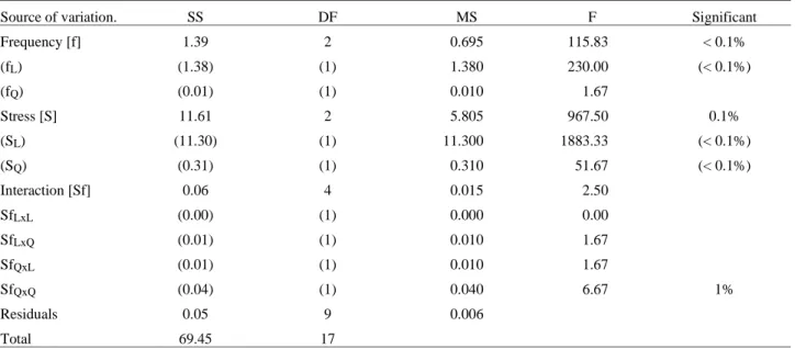
One can also use variance analysis to confirm the mag-nitude of the effects. This analysis is summarized in Table 5, which shows that the linear and quadratic components of stress in the total number of cycles to failure are highly significant. The SL component is relatively large in com-parison to the others, while frequency has a linear effect
Table 5.Analysis of the variance for the transformed data.
Source of variation. SS DF MS F Significant
Frequency [f] 1.39 2 0.695 115.83 < 0.1%
(fL) (1.38) (1) 1.380 230.00 (< 0.1%)
(fQ) (0.01) (1) 0.010 1.67
Stress [S] 11.61 2 5.805 967.50 0.1%
(SL) (11.30) (1) 11.300 1883.33 (< 0.1%)
(SQ) (0.31) (1) 0.310 51.67 (< 0.1%)
Interaction [Sf] 0.06 4 0.015 2.50
SfLxL (0.00) (1) 0.000 0.00
SfLxQ (0.01) (1) 0.010 1.67
SfQxL (0.01) (1) 0.010 1.67
SfQxQ (0.04) (1) 0.040 6.67 1%
Residuals 0.05 9 0.006
Total 69.45 17
Table 4.YATES’ algorithm of for the transformed data, of the Table 3.
i Y* Y*1 Y*2 D* E* Combination SQ
1 7.76665 25.5714 60.9134 18 3.38408 00 206.135
2 8.59402 21.4126 4.0664 12 0.33887 (**) 10 (fL) 1.378
3 9.21074 13.9294 -0.5338 36 -0.01483 20 (fQ) 0.008
4 6.42316 1.4441 -11.6420 12 -0.97017 (**) 01 (SL) 11.295
5 7.37327 1.1930 -0.0147 8 -0.00184 11 (SfLxL) 0.000
6 7.61613 1.4294 0.5947 24 0.02478 21 (SfQxL) 0.015
7 3.99247 -0.2106 -3.3243 36 -0.09234 (**) 02 (SQ) 0.307
interaction is significant at 1%, i.e., there is a slight inter-action between the two factors.
Observation 1:Currently there are many commercial computational programs for data analysis. The MINITAB V.10 was used in this study owing to several advantages it offers, such as its easy use, precision, and versatility of the different statistical techniques, among others.