i
Setembro, 2014
Frederico Paula Parreira
Licenciado em Ciências da Engenharia e Gestão Industrial
Antioxidant extraction process for Andean Oca by a
Photodiode Array Detector using Response Surface
Methodology
Dissertação para obtenção do Grau de Mestre em Engenharia e Gestão Industrial
Orientadora: Professora Doutora Ana Sofia Matos, Professora Auxiliar, Faculdade de Ciências e Tecnologia da Universidade Nova de Lisboa
Co-orientadores:
[], [Cargo], [Instituição]
[Nome do co-orientador 2], [Cargo], [Instituição]
Júri:
Presidente: Professora Doutora Virgínia Helena Arimateia de Campos Machado
i
Antioxidant extraction process for Andean Oca by a Photodiode Array Detector using
Response Surface Methodology
Copyright © Frederico Paula Parreira, Faculdade de Ciências e Tecnologia, Universidade Nova de Lisboa.
ii
iv
Agradecimentos
vi
Abstract
Application of Experimental Design techniques has proven to be essential in various research fields, due to its statistical capability of processing the effect of interactions among independent variables, known as factors, in a system’s response. Advantages of this methodology can be summarized in more resource and time efficient experimentations while providing more accurate results.
This research emphasizes the quantification of 4 antioxidants extraction, at two different concentration, prepared according to an experimental procedure and measured by a Photodiode Array Detector.
Experimental planning was made following a Central Composite Design, which is a type of DoE that allows to consider the quadratic component in Response Surfaces, a component that includes pure curvature studies on the model produced.
This work was executed with the intention of analyzing responses, peak areas obtained from chromatograms plotted by the Detector’s system, and comprehending if the factors considered – acquired from an extensive literary review – produced the expected effect in response. Completion of this work will allow to take conclusions regarding what factors should be considered for the optimization studies of antioxidants extraction in a Oca (Oxalis tuberosa) matrix.
viii
Resumo
A aplicação de técnicas de Desenho de Experiências provou ser essencial nos mais diversos campos de investigação, devido à sua capacidade estatística de processar o efeito de interações entre variáveis independentes, também conhecidas por fatores, na resposta produzida pelo sistema. As vantagens desta metodologia traduzem-se num aumento da eficiência de recursos e tempo experimental, produzindo ainda resultados com maior precisão.
Esta investigação foca-se na quantificação da extração de 4 antioxidantes, para duas concentrações diferentes, preparado de acordo com um procedimento experimental e medido por um Detetor de Fotodíodos.
O planeamento experimental foi concebido com base num Desenho do Compósito Central, um tipo de DoE que permite considerar a componente quadrática nas Superfícies de Resposta, componente essa que estuda a curvatura pura nos modelos produzidos.
Este trabalho foi realizado com a intenção de analisar as respostas, áreas de picos obtidas a partir de cromatogramas produzidos pelo Detetor, e compreender se os fatores considerados – adquiridos através de uma revisão literária extensiva – produziram o efeito esperado na resposta. O culminar deste estudo irá permitir tirar conclusões acerca dos fatores que devem ser considerados para os estudos de otimização da extração de antioxidantes numa matriz de Oca (Oxalis tuberosa).
x
Index
Introduction ... 1
Literature review ... 5
2.1.1. Full Factorial Design with two levels – 2k ... 6
2.1.2. Central Composite Design ... 14
2.2.1. Separation of compounds ... 20
2.2.2. Chromatograms: obtaining and analyzing results ... 21
Methodology and Results ... 27
3.1.1. Experimental results ... 29
3.1.2. Analysis of Variance ... 30
3.1.3. RSM and Contour plots ... 31
3.1.4. Regression Model ... 36
3.2.1. Experimental plan ... 39
3.2.2. Analysis of Variance ... 40
3.2.3. RSM and Contour plot ... 41
3.2.4. Regression Model ... 43
3.3.1. Experimental plan ... 44
3.3.2. Analysis of Variance ... 44
3.3.3. RSM and Contour Plot ... 45
3.3.4. Regression Model ... 48
xi
3.4.2. Analysis of Variance ... 49
3.4.3. RSM and Contour plots ... 50
3.4.4. Regression Model ... 53
Discussion/Conclusions ... 57
Bibliography... 58
Appendixes... 60
xii
Figures Index
Figure 2. 1 - Experimental procedure for a 2k Design... 7
Figure 2. 2 - Geometrical representation of a 2k Design ... 8
Figure 2. 3 - Normal Probability Plot of Raw Residuals ... 11
Figure 2. 4 - Predicted Values vs. Residual Values Graphic ... 11
Figure 2. 5 - Residuals vs. Case Numbers Plot ... 12
Figure 2. 6 - CCF Design representation for (a) 2 and (b) 3 factors ... 15
Figure 2. 7 - CCC Design representation for (a) 2 and (b) 3 factors ... 16
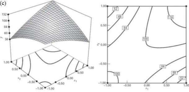
Figure 2. 8 - Response Surface Plot for (a) maximum (b) minimum and (c) saddle point .... 20
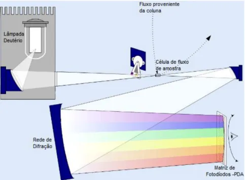
Figure 2. 9 - Representative scheme of a Photodiode Array Detector ... 25
Figure 3. 1 - RSM for Ellagic Acid (0,4mg/L): Acetonitrile x Column Temperature ... 32
Figure 3. 2 - Contour Plot for Ellagic Acid (0,4mg/L): Acetonitrile x Column Temperature 32 Figure 3. 3 - RSM for Ellagic Acid (0,4mg/L): Flux x Column Temperature ... 33
Figure 3. 4 - Contour Plot for Ellagic Acid (0,4mg/L): Flux x Column Temperature ... 33
Figure 3. 5 - RSM for Ellagic Acid (0,4mg/L): Flux x Acetonitrile ... 34
Figure 3. 6 - Contour Plot for Ellagic Acid (0,4mg/L): Flux x Acetonitrile ... 34
Figure 3. 7 - RSM for Ellagic Acid (4mg/L): Flux × Column Temperature ... 35
Figure 3. 8 - Contour Plot for Ellagic Acid (4mg/L): Flux × Column Temperature ... 36
Figure 3. 9 - Normal Probability Plot of Residuals for Ellagic Acid (0,4mg/L) ... 37
Figure 3. 10 - Predicted vs. Residual Values Plot for Ellagic Acid (0,4mg/L) ... 38
Figure 3. 11 - Residuals vs. Case Numbers for Ellagic Acid (0,4mg/L) ... 38
Figure 3. 12 - RSM for Ferulic Acid (0,2mg/L): Flux × Acetonitrile ... 41
Figure 3. 13 – Contour Plot for Ferulic Acid (0,2mg/L): Flux × Column Temperature ... 42
Figure 3. 14 - RSM for Ferulic Acid (2mg/L): Flux × Acetonitrile ... 42
Figure 3. 15 – Contour Plot for Ferulic Acid (2mg/L): Flux × Acetonitrile ... 43
Figure 3. 16 - RSM for Rutin (0,2mg/L): Flux × Column Temperature ... 46
Figure 3. 17 – Contour Plot for Rutin (0,2mg/L): Flux × Column Temperature ... 46
Figure 3. 18 - RSM for Rutin (2mg/L): Flux × Acetonitrile ... 47
Figure 3. 19 – Contour Plot for Rutin (2mg/L): Flux × Acetonitrile ... 48
Figure 3. 20 - RSM for Cinnamic Acid (0,2mg/L): Flux × Column Temperature ... 51
Figure 3. 21 – Contour Plot for Cinnamic Acid (0,2mg/L): Flux × Column Temperature .... 51
Figure 3. 22 - RSM for Cinnamic Acid (2mg/L): Flux × Acetonitrile ... 52
Figure 3. 23 - RSM for Cinnamic Acid (2mg/L): Flux × Acetonitrile ... 52
Figure 3. 24 – Highest RSM for low concentration standard: Ellagic Acid (0,4mg/L) ... 54
xiv
Tables Index
Table 2. 1- Design Matrix for a 23 full factorial ... 8
Table 2. 2 - Reduced Multi-Way ANOVA ... 13
Table 2. 3- Design Matrix for a Central Composite Design ... 17
Table 2. 4- Design Matrix for a Central Composite Design ... 18
Table 3. 1 - Experimental Factors and respective levels ... 27
Table 3. 2 - General Experimental plan ... 28
Table 3. 3 - Experimental plan and respective responses for Ellagic Acid solution ... 29
Table 3. 4 - ANOVA for 0,4 mg/L Ellagic Acid... 30
Table 3. 5 - Reduced ANOVA for 0,4mg/L Ellagic Acid ... 30
Table 3. 6 - Reduced ANOVA for 4mg/L Ellagic Acid ... 31
Table 3. 7 – Regression Coefficients for 0,4mg/L Ellagic Acid ... 36
Table 3. 8 - Experimental plan and respective responses for Ferulic Acid solution ... 39
Table 3. 9 - Reduced ANOVA for 0,2mg/L Ferulic Acid ... 40
Table 3. 10 - Reduced ANOVA for 2mg/L Ferulic Acid ... 41
Table 3. 11 - Experimental plan and respective responses for Rutin solution ... 44
Table 3. 12 - Reduced ANOVA for 0,2mg/L Rutin solution ... 45
Table 3. 13 – Reduced ANOVA for 2mg/L Rutin solution ... 45
Table 3. 14 - Experimental plan and respective responses for Cinnamic Acid solution ... 49
Table 3. 15 – Reduced ANOVA for 0,2mg/L Cinnamic Acid solution ... 50
Table 3. 16 - Reduced ANOVA for 2mg/L Cinnamic Acid solution... 50
xvi
List of Abbreviations
ANOVA Analysis of Variance
CCC Circumscribed Central Composite CCD Central Composite Design
DoE Design of Experiments OVAT One Variable At a Time
RSM Response Surface Methodology TAA Total Antioxidant Activity
TPC Total Phenolic Content
α Distance from center point to axial point β Regression coefficient
2k Two-level full factorial form
3k Three-level full factorial form
d.f. Degrees of freedom
eijk Residual for a particular experiment
E Ethanol concentration
k Factors
l Levels
lk Full factorial form
SS Sum of Squares
MS Mean Square
N Total number of experiments
n Number of replicas
nC Number of center points
R2 Coefficient of determination
xc Coded level
xmin Minimum real level
xmáx Maximum real level
1
Introduction
Contextualization
Throughout times the importance of statistical and mathematical models in life and decision making has taken a tremendous importance. Statistics is the mathematical science involving the collection, analysis and interpretation of data. While before this science used to be only applied to what could be called directly related fields, nowadays its usage is spread to various fields, because organizations and single individuals felt the need to stay on track with economical, technological and market demand. Its application can be found in diversified fields, such as Chemometrics, Business Analytics, Demography, Quality Control, Reliability Engineering, Quantitative Psychology, etc.
Chemometrics is the science of extracting information from chemical systems by data-driven means. It is a highly interfacial discipline, using methods frequently employed in core data-analytic disciplines such as multivariate statistics, applied mathematics, and computer science, in order to address problems in chemistry, biochemistry, medicine, biology and chemical engineering.
Chromatography is a chemical methodology used for separating compounds of a mixture and posterior analysis of concentrations. It was invented by Mikhail Tsvet on 1903, who used it to study the separation of plant pigments. Considered a powerful technology nowadays, it possesses a wide variety of techniques available for experimenters, allowing them to choose the most suitable processes for fulfilling the intended objective. Therefore, Chromatography plays an important role in many laboratorial researches and industrial applications (Ali et al. n.d.). An important activity in the Food certification process consists in quantifying all compounds concentrations present in the product, which will then be displayed in its label. Many companies hire the services of chemistry laboratories to separate and analyze these compounds, which is frequently made through chromatographic separation methods.
2
achievements became known internationally and started being applied in a global scale (Pereira & Requejo 2012).
Design Of Experiments filled in an important gap in the chemical field, by introducing a way that allows experimenters to study several parameters at the same time, demanding a smaller number of experiments, so consequently time and material were also reduced.
Motivation
This study intends to quantify the extraction process, by a Photodiode Array Detector, of four antioxidants using standards: Ellagic Acid, Ferulic Acid, Rutin and Cinnamic Acid. The success of this study is expected to lead to the quantification of this compounds for an Andean Oca (Oxalis tuberosa).
Experimental Design will allow to study the influence of Column Temperature, Flux and solvent concentration (% of Acetonitrile) in the extraction process. Supported by Response Surface Methodology (RSM) experimenters will be able to take conclusions regarding system’s response to the interaction of factors at different levels. Responses are quantified by the chromatographic peak areas obtained from the system being studied, the Photodiode Array Detector. An Analysis Of Variance will also inform if the alterations being made, to the independent variables that are considered to be important for this system, are responsible for response alterations.
Objectives
For the successful accomplishment of this thesis, the following objectives were determined:
Optimization of extraction process of antioxidants for the Oca matrix
Identification of the best significant factors combinations, and its respective levels, through the DOE methodology
Thesis structure
The present dissertation is organized in five chapters. The initial chapter contains a brief introduction to the thematic approached, stating this study’s objectives, the methodology used and this document’s structure.
3
Next chapter focuses on the Methodology used in this study, presenting the experimental plan and justifying the choices of factors, levels and Design. Furthermore, it includes the Analysis of Results for each of the four antioxidants studied: Ellagic Acid, Ferulic Acid, Rutin and Cinnamic Acid. In this part are examined all parameters considered to have importance for comprehending this study’s success.
5
Literature review
Design Of Experiments
Design of Experiments is a technique for discovering about new processes, acquire a better comprehension on existing products and optimizing these products/processes.
Design of Experiments (DoE) is a tool used for optimization of products or services, when correctly applied it can save time and money, along with other useful resources. Optimizing consists in improving the performance of a system, or process, in order to obtain the maximum benefit from it. It can be applied for products, services.
The DoE methodology was created by Sir Ronald A. Fisher in the 20s, who developed this statistical technique for agricultural purposes (Bhote 1999). Its scope only included enterprises after the improvements made by the Japanese Genichi Taguchi, who applied it first on his country, and later exported those ideas for eastern companies, turning it into a global scale methodology (Pereira & Requejo 2012).
In a Quality context, an experiment is a test that measures changes in system’s results, caused by overseen alterations in process’s input. Input variables, known as factors, are independent and may assume different values, the levels, these data may be of a quantitative or qualitative kind. Quantitative levels always need to be scalable (i.e. temperatures), while in the second case levels represent the variation of a condition, whether is to use or not an equipment, or trying out different materials in a process, etc. As a result of the procedure one or multiple responses, depending on the type of system, are obtained from each experiment. System’s performance is measured through comparison of changes in response values, as a reaction to factors’ manipulation. Hence, responses must be quantitative, in order to have well accurate and measurable indicators of optimization (Pereira & Requejo 2012).
Experimental design (DOE) is used with the purpose of studying the conformity of a characteristic(s), measured by response(s), to its expected value(s). Traditionally approaches on experimental studies were only about adjusting the average response. Although, this approach was limited and there was a need to know more about response’s behavior. Improvements were made so that variability in response, caused by factors, could be measured in order to take conclusions about which factors influenced response significantly, and the levels yielding better responses (Pereira & Requejo 2012).
6
the factors that revealed to have significant influence in response’s variability, to discover the levels yielding optimal response (Montgomery 2009).
Many enterprises, nowadays, utilize experimental designs in conception and development of new products, achieving major benefits in costs and time reductions by doing well at first. Also in Chemistry, it’s regularly applied, due to being an improvement in relation to traditional methods. Before the demystification of this statistical technique, optimization was carried out by monitoring the influence of One-Variable-At-a-Time (OVAT) on response, keeping the other variables at a fixed value. This approach depends on intuition, experience and luck for its success and even though is frequently unreliable and inefficient (Antony 2003). Comparing to this method, factorial designs have the benefit to investigate more than a factor per experiment, therefore obtaining in each response an estimation of several factors influence. It’s a more efficient option, demands less experiments to perform a complete study, and this efficiency level proportionally increases with the number of factors (Montgomery 2009).
2.1.1.
Full Factorial Design with two levels
–
2
kFull Factorial designs are one type of DoE represented by an lk exponentiation form. In
comparison with OVAT, it requires an inferior number of experiments, and allows to study when a factor’s effect on response is altered by a different level of another factor, known as interaction. This exponentiation indicates the total number of experiments that need to be performed to study k factors (exponent) at l different levels (base). Replication of experiments is the act of repeating the original experimental conditions for several sets of samples n. It’s used to estimate experimental error and also allows a more accurate estimation of factors/interactions effects. The total number of experiments is expressed by N = n × lk. All factors are included in each experiment
and studied for the same number of levels (Pereira & Requejo 2012; Montgomery 2009; Antony 2003). During this work only the 2k basis structure will be approached, although full factorials can also be created for three levels (3k designs).
For an easier display, it was established that factors would be represented by capital letters, according to the alphabetic order. Experimental levels are assigned with codified levels of xc=+1
(or “+”) and xc=-1 (or “-”), known as high and low levels. The relation between coded (xc) and
experimental levels (x) is given by Equation 2.1. Previous to the experiments, researcher needs to assign these codes to experimental values (Pereira & Requejo 2012).
𝑥𝑐=
𝑥 − (𝑥𝑚𝑎𝑥+ 𝑥𝑚𝑖𝑛) 2 (𝑥𝑚𝑎𝑥− 𝑥𝑚𝑖𝑛)
2
7
Experimental Plan
Experiments are planned according to a specific non-randomized order, called “standard order” (or Yates order). This procedure can be accomplished by following sequential instructions described:
A Design Matrix (Table 3) is a visual representation of the experimental plan. Initial experiment (step 1) tests all factors at a low level, and is represented by “(1)” in the matrix. Next, a factor chosen according to priority criteria (Factor A) – alphabetic order – is set at high level, all others are set to low level, and experiment “a” is introduced in the plan (steps 2 and 3). Researcher then proceeds to a verification (step 4), if there are other experiments with high level factor(s) already planned, although yet to be combined with the one just planned, if so those combinations are next in plan (step 5). Otherwise, next factor in list enters the plan. This procedure is repeated until all factors and combinations are inserted in the plan. Coefficients “+” and “–” in the Matrix represent the levels, high or low, that factors are set. Design matrix displayed is a 23
Factors Level +
Level -
Units Factor A 120 60 ºC Factor B 50 100 min
Factor C 20 30 Atm
1st Experiment – All factors tested at low level
Select next factor in list (alphabetical order)
Set only the selected factor at
high level, remaining are set low New experiment planned
Combination not studied?
New experiment planned Set both uncombined factors at
high level
1
2
3
4
5 Y
N
8
full factorial with all interactions AB, AC, BC and ABC. This experimental region can also be geometrically represented by a cube (Fig. 2).
Number of replications n indicates how many times the whole set of experiments is ran under equivalent experimental conditions. Replica is the name given to an individual response that is replicated. It’s possible to observe there are two sets of responses (n=2) in Table 1, yx1 and yx2.
Table 2. 1- Design Matrix for a 23 full factorial
Factors Response
Standard Order
A B C
(1) – – – y11
y12 …
y1N
a + – –
b – + –
ab + + –
c – – +
ac + – +
bc – + +
abc + + +
Figure 2. 2 - Geometrical representation of a 2k Design
By fulfilling these obligatory requirements, a matrix is automatically orthogonal. This characteristic verifies if (Pereira & Requejo 2012):
In each column the number of low levels (-) is the same as the number of high levels (+);
9
The columns are orthogonal given that the sum of any coefficients’ product (product of any two columns) will always equals zero;
A column multiplied by itself results in the identity column, which is composed only by + signs in the matrix;
The product of any two columns results always in other column of the matrix.
Regression Model
From a factorial design it’s possible toproduce a regression model predictive of system’s response. All factors and interactions are initially considered to be part of this model, and for that reason it’s called a full model (Eq. 2.2). For a 23 design, average of total responses is measured by β0– also called the intercept –, regression coefficients, β1 to β123, measure the effect on response
y given by a unit alteration in factor/interaction’s level. Variables x1 to x3 represent the codified
levels, although, they can also be replaced by experimental values by means of Eq. 2.1. Including more factors increases the number of regression coefficients and codified variables. With the results achieved from the multi-way ANOVA, a model can be built with only the significant factors and/or interactions, eliminating from the equation all other components.
𝑦̂ = 𝛽̂0+ 𝛽̂1𝑥1+ 𝛽̂2𝑥2+ 𝛽̂3𝑥3+ 𝛽̂12𝑥1 𝑥2+ 𝛽̂13𝑥1𝑥3+ 𝛽̂23𝑥2 𝑥3+ 𝛽̂123𝑥1𝑥2 𝑥3+ 𝜀
In this model there are main effects, used to estimate linear responses, and interaction effects, used to estimate small curvature responses. A 2k regression model can only go this far, not being able to yield good estimates of highly curved responses. In the next subchapter will be presented a method more fit for this type of response surfaces.
Calculus of Effects
A contrast is the total sum of responses obtained by a factor, or interaction of factors. Responses (y1 to yN) are multiplied by the respective coded levels (x1 to xN) and summed (Eq. 2.3).
This information can easily be extracted from Design Matrix’s columns.
𝐶𝑜𝑛𝑡𝑟𝑎𝑠𝑡𝑋 = 𝑥1𝑦1+ 𝑥2𝑦2+ ⋯ + 𝑥𝑁𝑦𝑁
Experimenter’s intention is to prove that variation in response derives from factors’ manipulation, and therefore must be measured. So the influence in response attained from changing a factor’s level is called an effect. There are main and interactive effects, first refers to changes in a single factor’s level while the second is due to changes in interaction’s levels(Antony 2003; Montgomery 2009; Pereira & Requejo 2012). A generalized equation is used to represent effects:
10 Effect𝑋 = 𝐶𝑜𝑛𝑠𝑡𝑟𝑎𝑠𝑡 𝑋2𝑘−1× 𝑛
Model Validation
A regression model can only be tested for variance if certain assumptions are fulfilled. These assumptions are that responses must be normally distributed, factors must be independent variables and system’s variance must be constant. Several tests can be applied to verify these assumptions, although through an analysis of residuals is possible to confirm all of them.
A residual (Eq. 2.5), calculates the difference between one experiment’s response and the average of responses.
𝑒𝑖𝑗𝑘 = 𝑦𝑖𝑗𝑘− 𝑦̅𝑖𝑗𝑘
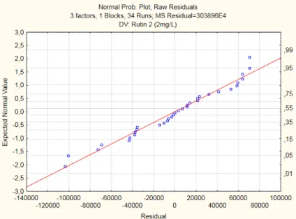
A normal probability plot of residuals can be used to verify the normality assumption, although an examination of standardized residuals (Eq. 2.6) is required to check for outliers. Approximately 68% of these values should fall within the limits ±1, about 95% of them in ±2, and all of them in ±3. If standard residuals are approximately according to these percentages it means that there aren’t outliers (Montgomery 2009).
𝑑𝑖𝑗𝑘= 𝑒𝑖𝑗𝑘 √𝑀𝑆𝑅𝑒𝑠𝑖𝑑
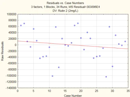
In order to verify the independence of variables and constant variance assumption, residuals are plotted vs. the run order of time and vs. the fitted value. If a particular tendency can be observed in these graphics then it’s likely for these assumptions to be broken. Summing up, no obvious patterns or tendencies can be found in residuals plots for assumptions to be verified (Montgomery 2009).
(2.4)
(2.5)
11
Figure 2. 3 - Normal Probability Plot of Raw Residuals
12
Figure 2. 5 - Residuals vs. Case Numbers Plot
Analysis of Variance
Variation in response caused by a factor or interaction is measured by the Sum of Squares, SSX
(Eq. 2.7). Total system’s variation SSTotal (2.8) is the sum of variation explained by factors and its
interactions SSModel, while the variation caused by other variables not accounted in the system is SSResid. The total variation can also be expressed by the sum of each response’s square value minus the square of all responses dividing by the total number of experiments.
𝑆𝑆𝑋= (𝐶𝑜𝑛𝑠𝑡𝑟𝑎𝑠𝑡 𝑋) 2 2𝑘× 𝑛
𝑆𝑆𝑇𝑜𝑡𝑎𝑙 = 𝑆𝑆𝑀𝑜𝑑𝑒𝑙+ 𝑆𝑆𝑅𝑒𝑠𝑖𝑑𝑢𝑎𝑙= ∑ ∑ ∑ 𝑦𝑖𝑗𝑘2 𝑛 𝑘=1 2 𝑗=1 2 𝑖=1
−(∑2𝑖=1∑2𝑗=1∑𝑛𝑘=1𝑦𝑖𝑗𝑘) 2
2𝑘𝑛
Mean Square, MSX, is an estimative of system’s variance that measures variability explained by a factor or interaction. Variability that isn’t explained by the model is given by MSResid.
𝑀𝑆𝑋 = 𝑆𝑆1𝑋
𝑀𝑆𝑅𝑒𝑠𝑖𝑑 = 2𝑘𝑆𝑆× (𝑛 − 1)𝑅𝑒𝑠𝑖𝑑
(2.7)
(2.8)
(2.9)
13
A multi-way ANOVA is a statistical tool used to test the significance of model’s dependent variables through a Fischer exact test. A Fischer test compares a statistic F0 to a critical value, Fα;d.f. Model; d.f. Resid obtained from a Fischer distribution. Two possible conclusions can be taken:
Factor/interaction is significant if F0 > Fα;d.f. Model; d.f. Resid Factor/interaction is insignificant if F0 < Fα;d.f. Model; d.f. Resid
𝐹0 =𝑀𝑆 𝑀𝑆𝑋 𝑅𝑒𝑠𝑖𝑑
An ANOVA table is used to summarize information regarding model’s significance. Factors that don’t have significant influence should be removed and put on the variation that isn’t explained by the model, SSResid. From this changes made, a reduced ANOVA containing only significant factors can be built (Table 2). In case significant factors are altered by this reduction, measures should be taken to address this problem. Model’s reduction causes a division of residual variance in two components, SSPure Error, resultant from factorial experiments, and SSLack of Fit, resultant from non-significant variables excluded from the model.
Table 2. 2 - Reduced Multi-Way ANOVA
After discovering the significant factors, an assessment of effects must be done to take conclusions regarding which experimental values yield better responses. Effect’s magnitude tells which factor influence more response, while direction gives information on which levels to choose. Summarizing, it’s the combination of ANOVA and effects that allow to learn more about the experimental values that are representative of the system.
For scenarios in which replication occurs (n≥2), as the one demonstrated, it’s possible to create an estimation of the residual variation. Although, it’s not always possible to conduct replication experiments. Limited resources, budget and time may appear as obstacles to it.
To verify if responses estimated by the model are in accordance with system’s production, measures as R2 and R2adj are used. Both parameters measure the total percentage of response
Source of variation
SS d.f. MS F0
A SSA 1 𝑆𝑆
1
𝑀𝑆𝐴 𝑀𝑆𝑅𝑒𝑠𝑖𝑑
AC SSAC 1 𝑆𝑆
1
𝑀𝑆𝐴𝐶 𝑀𝑆𝑅𝑒𝑠𝑖𝑑
ABC SSABC 1 𝑆𝑆
1
𝑀𝑆𝐴𝐵𝐶 𝑀𝑆𝑅𝑒𝑠𝑖𝑑 Residual SSResid 2k(n-1)+d.f.insig. 𝑆𝑆
𝑑. 𝑓.𝑅𝑒𝑠𝑖𝑑
14
estimated by the model, although the R2adj is considered more reliable due to having a better adjustment to non-significant factors.
𝑅2 =𝑆𝑆𝑀𝑜𝑑𝑒𝑙 𝑆𝑆𝑇𝑜𝑡𝑎𝑙
𝑅2
𝑎𝑑𝑗.= 1 −
𝑆𝑆𝑅𝑒𝑠𝑖𝑑 𝑑. 𝑓.𝑅𝑒𝑠𝑖𝑑
𝑆𝑆𝑇𝑜𝑡𝑎𝑙 𝑑. 𝑓.𝑇𝑜𝑡𝑎𝑙
2.1.2.
Central Composite Design
A Central Composite Design is used to study a region of interest larger than the one confined between two factorial levels. It’s highly used in optimization experiments when standard factorial designs can’t reach optimal solutions. Designs are built from a factorial structure, to which central and axial experiments are added (Hibbert 2012; Ferreira et al. 2007). The Composite experiments for a two-level full factorial can be described by:
𝑁 = 2𝑘+ 2 × 𝑘 + 𝑛 𝑐
As expressed in the equation, experiments can be divided in three sequenced block. The first one is a full factorial design (2k), in which factors are tested at two levels, which are selected by
researchers from previous screening experiments, or alternatively from performing a literary review. A second block (nc) is added, in which a new level centered between the two factorial
levels is generated, it’s codified as x=0. For this block to be created all factors need to be quantitative (Ferreira et al. 2007). Several experiments are performed in this point, where all factors possess the same codified level, called the centerpoint of the design region. The number of centerpoint replications, nC, is established by the researcher according to criteria that will be further explained with more detail.
Axial experiments (2×k), represented by the 3rd block are dependent on an evaluation of system’s curvature. If the test proves that curvature is significant, should be added to the design. An analysis of variance is applied for that purpose:
𝑆𝑆𝐶𝑢𝑟𝑣𝑎𝑡𝑢𝑟𝑒=𝑛𝐹𝑛𝐶𝑃(Ȳ𝐹− Ȳ𝐶𝑃) 2 𝑛𝐹+ 𝑛𝐶𝑃
𝑀𝑆𝐶𝑢𝑟𝑣𝑎𝑡𝑢𝑟𝑒 = 𝑆𝑆𝐶𝑢𝑟𝑣𝑎𝑡𝑢𝑟𝑒1
(2.12)
(2.13)
(2.14)
(2.15)
15 𝑀𝑆𝐸𝑟𝑟𝑜𝑟 = ∑ (𝑦𝑗− Ȳ𝑐𝑝)
2 𝑛𝑐𝑝
1
𝑛𝑐𝑝− 1
Where ῩF and ῩCP represent the average response for factorial and centerpoint experiments,
while nF and nCP stand for the number of experiments made for each block. Using the Fischer
exact test (Eq. xx) it’s possible to verify if curvature is significant. If significance is verified, axial experiments are performed creating two new levels, codified as x=α and x=-α. The parameter α represents the distance between axial level and centerpoint level.
It’s possible that sometimes experimenters don’t use this test, and instead take a conservative approach considering that curvature might exist and therefore performing a complete CCD, with the three blocks.
Design Features
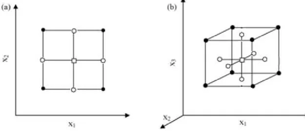
According to the requirements of the system investigated, researcher needs to define two main features to characterize a design, the distance from axial level to the center of design (α) and the number of replications (nC) at the centerpoint (Montgomery 2009). For a cubical region of interest a center faced design (CCF) can be applied, this design features are α=1 and a small number of replications at the center, usually one or two (Ferreira et al. 2007).
Figure 2. 6 - CCF Design representation for (a) 2 and (b) 3 factors
16
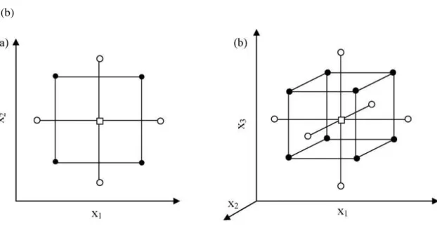
estimates of variance depend exclusively on their distance to the design centerpoint, making the precision of predicted response be the same for all points located in the hypersphere around the design center. For this reason, the distance from axial points and factorial points to the center of the design has to be equal, generating a hypersphere region (Montgomery 2009; Ferreira et al. 2007). This rotatability is verified for:
𝛼 = 2𝑘/4
Creating a circumscribed design for the biggest axial distance (α=√k) demands a consequently higher number of centerpoint replications, because the growth of experimental error increases with the experimental region.
Figure 2. 7 - CCC Design representation for (a) 2 and (b) 3 factors
Selecting α depends mainly on the type of response system is expected to generate, while the number of centerpoint replications is chosen according to α and the accuracy of experimental error intended, it produces an independent estimative of this error without changing estimative of effects (Pereira & Requejo 2012).
Experimental Plan
Experimental planning is displayed by means of a Design Matrix divided in three parts. Factorial component is the first subset of experiments that appears on the design, it’s composed by the first 8 experiments, followed by centerpoint replications in which all factors are set at the same level “0”. Axial experiments are the last component added, two experiments are performed (2.18)
17
for each factor studied, one at the high level “α”, and the other at the low level “-α”. Remaining factors, not set for axial levels, are all fixed at level “0”(Montgomery 2009).
Defining the levels with clarity is crucial to attain a successful optimization (Baş & Boyacı 2007). The proximity of experimental values can compromise response’s variation, not causing enough variation to have a clear distinction between different levels responses (Hibbert 2012).
Calculus of Effects and Analysis of Variance
The main difference from the Central Composite Design to the Full Factorial Design is the ability to include pure curvature in its model. Therefore, in its ANOVA are included the square factors such as it’s demonstrated under.
Factors Standard
Order
A B C
1 –1 –1 –1
2 +1 –1 –1
3 –1 +1 –1
4 +1 +1 –1
5 –1 –1 +1
6 +1 –1 +1
7 –1 +1 +1
8 +1 +1 +1
9 0 0 0
10 0 0 0
11 0 0 0
12 1,682 0 0
13 -1,682 0 0
14 0 1,682 0
15 0 -1,682 0
16 0 0 1,682
17 0 0 -1,682
Factorial Component
Central Component
Axial Component
18
Regression Model
A regression model to study pure curvature applies for cases in which there’s indication of significant curvature. In that case, the model is given by:
𝑌 = 𝛽0+ ∑ 𝛽𝑖𝑥𝑖 𝑘
𝑖=1
+ ∑ ∑ 𝛽𝑖𝑗𝑥𝑖𝑥𝑗 𝑘
𝑗>𝑖 𝑘
𝑖=1
+ ∑ 𝛽𝑖𝑖𝑥𝑖2 𝑘
𝑖=1
+ 𝜀
This model can be reduced to only the significant components after running the multi-way ANOVA.
Response Surface Methodology
A Response Surface Methodology is a set of statistical techniques used to develop a surface that reflects the response system is expected to return, produced by a regression model, to changes in factors’ levels. This tool is used by statistical computer softwares that allow to process a bigger amount of information faster. According to Montgomery “the eventual objective of RSM is to determine the optimum operating conditions for the system or to determine a region of the factor space in which operating requirements are satisfied” (Montgomery 2009).
It starts by using techniques to improve response produced by a first-order model, by increasing or decreasing it until the maximum/minimum response that this model can produce. These responses are attained through the method of the steepest ascent for increasing response, and method of the steepest descent to decrease it. A second-order model is then used to find the optimum, this point can be a maximum, minimum or saddle point. This point is known as stationary point and it’s located where partial derivatives ∂ŷ/∂x1=∂ŷ/∂x2=∂ŷ/∂xk=0.
Source of variation
SS d.f. MS F0
A SSA 1 𝑆𝑆
1
𝑀𝑆𝐴 𝑀𝑆𝑅𝑒𝑠𝑖𝑑
B SSB 1 𝑆𝑆
1
𝑀𝑆𝐵 𝑀𝑆𝑅𝑒𝑠𝑖𝑑
AB SSAB 1 𝑆𝑆
1
𝑀𝑆𝐴𝐵 𝑀𝑆𝑅𝑒𝑠𝑖𝑑
A2 SSA2 1 𝑆𝑆
1
𝑀𝑆𝐴2
𝑀𝑆𝑅𝑒𝑠𝑖𝑑
B2 SSB2 1 𝑆𝑆
1
𝑀𝑆𝐵2
𝑀𝑆𝑅𝑒𝑠𝑖𝑑
Residual SSResid ncp -1 𝑆𝑆
𝑑. 𝑓.𝑅𝑒𝑠𝑖𝑑
19
20
Figure 2. 8 - Response Surface Plot for (a) maximum (b) minimum and (c) saddle point
Chromatography
Chromatography is a chemical method used for separating compounds that are mixed in a solution. Usually, the procedure is separated in three chronological stages, sample preparation, analysis of compounds and analyte extraction. All chromatographic processes have at least two points in common: a solvent designated as mobile phase that passes through the mechanism, and a stationary phase that retains compounds temporarily. The interaction of these two phases can be used to classify the different methods used. In Column Chromatography, the stationary phase is fixed in a tube and the mobile phase is forced to pass through this tube, while in Plain Chromatography the stationary phase is supported by a plaque or by a paper, and the mobile phase passes through it by capillarity or with the help of gravity. The other way to classify it is according the type of mobile phases used: gas chromatography, liquid chromatography and supercritical fluid chromatography (Gonçalves 2001).
2.2.1.
Separation of compounds
Compounds in a mixture can be separated through diverse techniques, such as normal phase chromatography, liquid-liquid partition chromatography, reversed phase chromatography, ion exchange chromatography, etc.
21
polar components are attracted to the stationary phase. Polarity is the characteristic used by the separation mechanism by this method (Meyer 1988).
2.2.2.
Chromatograms: obtaining and analyzing results
After the solid-mobile phase interaction, separated compounds are sent to the mass detector which registers an electrical sign, this sign is sent to the computer and displayed graphically as a Chromatogram. A chromatogram is a graphic containing Gaussian curves, also known as peaks, which supply qualitative and quantitative information about the mixture. Retention time is a qualitative information represented by the time separating injection moment, from the moment when signal maximum is reached, and it’s only obtained under identical chromatographic conditions: column dimensions, type of stationary phase, mobile phase composition and flow velocity. When these variables are repeatedly experimented with the same values, it’s possible to identify a peak through retention times’ comparison.
Compounds main data that can be retrieved from a chromatogram is the peak width, w1,at the
baseline, and the dead time, t0, or time required by the mobile phase to pass through the column.
Quantitative information such as areas and concentrations of compounds can be calculated from graphic parameters, this data is used to establish comparisons between compounds and take conclusions regarding separation’s efficiency.
Response Surface Methodology applied to antioxidant extraction
The usage of RSM as a support to investigate the statistical importance of various variables in a response as revealed itself fundamental. From its advantages, the one that must be underlined is its capacity of studying curvature in models by plotting the response surface, a three dimensional representation of the effect caused by two independent variables in a dependent variable.
An appropriate selection of factors has a crucial role in experimental success, and there are two paths that can be followed to arrive to conclusions:
Screening experiments – A set of experiments is performed according to an experimental design, in which all factors that might be important of factors should be considered. The experimental goal is to reduce the number of factors to only the significant ones.
22
Ideally both tasks should be materialized in order to achieve a successful optimization, even if sometimes it’s not possible due to being time and resource constraining.
State-of-the-Art Review
In order to optimize the Total Phenolic Compounds extraction and antioxidant activity on fresh dark figs, an experimental design was done. The factors considered were temperature (25-65ºC), time (60-120 min) and acetone concentration (40-80%). Box-Behnken was the design selected for these experiments, due to a need of studying factors at 3 levels each.
Experimenters concluded that all factors considered influenced significantly TPC and antioxidant activity of fig extracts. The optimal conditions to obtain the highest extraction of phenolics from fresh dark fig, as well as maximum antioxidant activity, were acetone concentration of 63.48%, temperature of 48.66 ºC, and extraction time of 115.14 min. Under optimal conditions, the experimental values for TPC and antioxidant activity were 536.43 ± 5.53 and 68.77 ± 1.43 mg GAE/100 g DM, respectively. These experimental results were in agreement with the predicted values which corresponding to 540.10 mg and 71.86 mg GAE/100 g DM (Bachir Bey et al. 2014).
A solid-liquid extraction process was optimized using a Response Surface Methodology for three factors: Temperature, pH and Ethanol concentration. The design applied for this optimization was a Central Composite, in the form: 23+2×3+6. This optimization was conducted for Pyracantha fortuneana fruits with a focus on total phenolic content (TPC) and total antioxidant activity (TAA). Based on the ANOVA, experimenters gauged that EtOH concentration, extraction temperature, and solution pH had significant positive linear effects on antioxidant activity, whereas their quadratic interaction had significant negative effects on TAA. Extraction conditions for optimized responses were EtOH = 71%, T = 51 ºC, and pH = 3.2. The maximum TAA predicted by contour plots was 1755 U/g dried PFF sample weight, whereas the value in our results under the optimum conditions was 1728 ± 14 U/g dried sample weight(Zhao et al. 2013).
Optimal conditions for antioxidant extraction from potato peel waste in a HPLC system were studied using a Response Surface Methodology. The extraction of antioxidants as a function of Temperature (T), Ethanol concentration (E) and Time (t) was studied using a rotatable second order design (CCD) with six replicates– 23 + 2x3 + 6 – in the centre of the experimental domain, and therefore α = 1,681. The conditions of the independent variables studied ranged from 25-90ºC for T, 20-100% for E and t between 5-150 min. The main phenolic compounds identified in the extracts were chlorogenic (Cl) and ferulic (Fer) acids. (Amado et al. 2014).
23
extraction (MAE) and the independent variables considered were extraction time (ET), liquid-to-solid ratio (LSR), and microwave power (MWP). A central composite design was used and a total of 30 experiments was performed (Ranic et al. 2014). The investigated factors, Extraction Time and Ethanol percentage, ranged from 40s to 360s and 20% to 80% (v/v) respectively. Deriving from these factors combination, the total extract yield ranged from 7.694 to 31.216 mg/g d.w SCG. The maximum yield was recorded on the 24th run, under following experimental conditions: 180s, 12 ml/g, and 550W MWP. Concerning the Total Phenolic Content (TPC) expressed in percentage (%, w/w) of dry SCGE, the yield ranged from 18.83 to 79.83%. The maximum yield was recorded in sample run 16, for the following levels: 40s, 240 W MWP and 6 fold solvent to SCG ratio(Ranic et al. 2014).
Extraction conditions for Mangifera Pajang peels were optimized through a Response Surface Methodology. System’s performance was measured in terms of total phenolic content and antioxidant capacity, and the variables studied were solvent concentration (ethanol), extraction temperature and liquid-to-solid ratio. A total of 20 experiments, divided in 8 factorial plus 6 star points and 6 center points, were performed following a central composite design. Three optimal conditions were developed for the responses, which were ethanol concentration 68%, 55 ºC and 32.7 mL/g, for TPC generating a response of 14.6 mg GAE/g, while for AC it was 68%, 56 ºC and 31.8 mL/g with a response of 0.2065 nm.(Prasad et al. 2011).
The Subcritical water extraction method was optimized for seeds of Coriandrum sativum. The parameters measured were the total phenolics and total flavonoids, which were conditioned by temperature (100-200º C), pressure (30-90 bar), and extraction time (10-30 mins). The experimental design applied for this case was a Box-Behnken with 3 factors and 3 levels (Zeković et al. 2014).
24
Oca Tuber
The Oca is an amylase tuber that grows in the Andean regions, especially in Peru and Bolivia, which is very similar to a potato and can be visually distinguished by two characteristics: shape and color. The second most widely cultivated native tuber in the Andes is Oxalis tuberosa, which belongs to the Oxiladaceae family. It’s actually harvested as a substitute product of the common potato, given its similar nutritional value and the fact that they are more resistant to plagues and diseases. It’s a culture that easily grows in poor soils and adverse climacteric conditions (Alcalde-eon et al. 2004).
The phytopharmaceuticals that are applied in the harvesting have a beneficial effect for the end consumer, due to the antioxidants compounds present that prevent several human deceases such as cardiovascular deceases, cancer and oxidant stress. Therefore, it’s important to quantify the presence of these compounds in food. These type of experiments, that provide information regarding aliment’s characteristics, assume a major importance for health organizations that can than approach nutritional problems of the local cultures with more knowledge. It allows them to develop nutritional plans and campaigns based on reliable information(Chirinos et al. 2009).
Photodiode Array Detector
These detectors can detect any light absorption from the ultraviolet region (190 nm) until the visible region (720 nm). Its biggest advantage is to allow experimenters to monitor a wide range of wavelengthsat once. Consequently, it provides benefits such as reduction of run time and solvent expenditure (Meyer 2010).
25
27
Methodology and Results
This study was designed with the objective of identifying the factors influencing the extraction process, using a Photodiode Array Detector system, for four antioxidants: Ellagic Acid, Ferulic Acid, Rutin and Cinnamic Acid. In order to characterize the antioxidants were used the standards of each compound. Except for Ellagic Acid, standards applied had two concentrations: 0,2mg/L and 2mg/L. The reason for using different standards for the first antioxidant – 0,4mg/L and 4mg/L – is that in previous experiments made, the researchers observed that the standards previously defined weren’t producing responses.
Experimental Plan
The experimental plan was made according to DoE methodology, more specifically a Central Composite Design (CCD) was the option selected due to giving the possibility of including pure curvature studies in its predictive model. The factors considered for this study were: the Column Temperature in ºC, the Solvent Concentration in % of Acetonitrile, and the Flux in ml/min. These were the independent variables considered by the researchers to have an important influence over the dependent variable extraction, which is measured in Peak Area (system’s response).
A total of n= 17 experiments were performed with two replicas for each standard solution as shown:
Factors Level
-1,682 Level - 1 Level 0 Level +1 Level +1,682 Units Column Temperature
30 34 40 46 50 ºC
Dissolution Solvent
1 21 50 79 99 % Acetonitrile
Flux 0,20 0,25 0,33 0,40 0,45 ml/min
28
Table 3. 2 - General Experimental plan
Factors
Standard
Order
A B C
1 34 21 0,25
2 46 21 0,25
3 34 79 0,25
4 46 79 0,25
5 34 21 0,40
6 46 21 0,40
7 34 79 0,40
8 46 79 0,40
9 40 50 0,33
10 40 50 0,33
11 40 50 0,33
12 50 50 0,33
13 30 50 0,33
14 40 99 0,33
15 40 1 0,33
16 40 50 0,45
17 40 50 0,20
The number of experiments isn’t sorted randomly, it results from a quantitative and a qualitative analysis made by the experimenters relaying mainly on how accurately we need to comprehend the system. If the system requires a light comprehension due to the requirements of its practical application being low, not demanding precision in response then a standard experimental design can be enough, such as a two level full factorial (2k) or fractional factorial (2k-p). The three level experiments (3k or 3k-p) aren’t commonly considered because they demand a high number of experiments to study few factors, achieving easily an unbearable number of experiments giving the exponential characteristic of factorial experiments. Therefore when laboratorial resources are strictly limited, or when the time is crucial, this option is not valid.
For this experiment, the more suitable option was a Central Composite Design with 3 centerpoint experiments – N= 23+ 2x3 + 3= 17 experiments. This experimental plan allows to retrieve information regarding the curvature of the system, allowing to produce a predictive model that includes linear components, interaction components and quadratic components.
29
Ellagic Acid
3.1.1.
Experimental results
A set of 17 solutions were prepared for two different concentrations of Ellagic Acid standard – therefore achieving a total of 34 experiments – subject to variations in Column Temperature, Flux and Acetonitrile Concentration. The first experimental set was prepared using a standard concentration of 0,4mg/L, while the second was made using a 4mg/L concentration. The solutions were then inserted into the Photodiode Array Detector and responses were measured in peak areas, as shown in Table 3.3. The highest extractions for both Ellagic Acid standards were achieved on the 3rd experiment, in which peaks of 52939 and 53424 were observed for the two low standard replicas, while 402019 and 427993 were the peaks for the high standard replicas. Consequently, it’s possible to observe that the real experimental conditions yielding best results are: 34ºC, 79%, and 0,25 ml/min.
Table 3. 3 - Experimental plan and respective responses for Ellagic Acid solution
Responses
Factors 0,4 mg/L 4 mg/L
Std.
Order
A B C 1st
Injection 2nd Injection 1st Injection 2nd Injection
1 34 21 0,25 33428 31926 323043 327177
2 46 21 0,25 32031 30902 298781 307117
3 34 79 0,25 52939 53424 402019 427993
4 46 79 0,25 28712 30550 217184 240422
5 34 21 0,40 11800 12520 118842 124667
6 46 21 0,40 10327 10330 122451 127954
7 34 79 0,40 18175 18722 64399 62685
8 46 79 0,40 14081 15276 50704 50497
9 40 50 0,33 21572 20240 223849 234490
10 40 50 0,33 27384 25872 129708 214036
11 40 50 0,33 10895 11294 33186 34154
12 50 50 0,33 5274 5335 41592 44819
13 30 50 0,33 9121 9902 53093 91611
14 40 99 0,33 20681 23761 215023 236036
15 40 1 0,33 18699 19523 186780 192124
16 40 50 0,45 17339 17849 176084 179993
30
3.1.2.
Analysis of Variance
Ellagic Acid (0,4 mg/L)
The Analysis of Variance obtained for an Ellagic Acid low standard (0,4mg/L) is represented in Table 3.4. Significant factors are identified with the bold effect, therefore it’s possible to observe that these factors are: Column Temperature (Linear), Column Temperature (Quadratic), Acetonitrile (Linear) and Flux (Linear). The last factor is the one that has higher influence (p=0,000002) in response for this low standard compound. It’s imperative to perform an ANOVA Reduction to verify if by fitting other non-significant factors in the Error, more factors will become significant.
Table 3. 4 - ANOVA for 0,4 mg/L Ellagic Acid
Var.:Ellagic Acid 1 (0,4 mg/L)
SS df MS F p
Column Temp. (ºC) (L) 2,341469E+08 1 2,341469E+08 4,92115 0,036243
Column Temp. (ºC) (Q) 4,271174E+08 1 4,271174E+08 8,97687 0,006263
Acetonitrile (%) (L) 2,232602E+08 1 2,232602E+08 4,69234 0,040452
Acetonitrile (%) (Q) 2,989626E+07 1 2,989626E+07 0,62834 0,435731
Flux (ml/min) (L) 1,860561E+09 1 1,860561E+09 39,10404 0,000002
Flux (ml/min) (Q) 5,480615E+07 1 5,480615E+07 1,15188 0,293829
1L by 2L 1,473614E+08 1 1,473614E+08 3,09714 0,091172
1L by 3L 9,177161E+07 1 9,177161E+07 1,92880 0,177645
2L by 3L 1,612223E+07 1 1,612223E+07 0,33885 0,565924
Error 1,141914E+09 24 4,757976E+07
Total SS 4,306910E+09 33
Displayed in Table 3.5, the Reduced ANOVA shows that this procedure didn’t acquire any new significant factors. As a result, it’s possible to state that 4 factors had significant influence in 0,4mg/L Ellagic Acid standard.
Table 3. 5 - Reduced ANOVA for 0,4mg/L Ellagic Acid
Var.: Ellagic Acid (4 mg/L)
SS df MS F p
Column Temp. (ºC) (L) 2,341469E+08 1 2,341469E+08 4,47855 0,043027
Column Temp. (ºC) (Q) 4,727691E+08 1 4,727691E+08 9,04270 0,005402
Acetonitrile (%) (Q) 2,232602E+08 1 2,232602E+08 4,27032 0,047816
Flux (ml/min) (L) 1,860561E+09 1 1,860561E+09 35,58713 0,000002
Error 1,516173E+09 29 5,228184E+07
31
Through an analysis of the coefficient of determination, R2= 0,64797, we can verify that for Ellagic Acid (0,4mg/L) the regression model approximates the real data.
Ellagic Acid (4 mg/L)
The Reduced ANOVA (Table 3.6) made for the Ellagic Acid 4mg/L standard demonstrates that Column Temperature (Q), Acetonitrile (Q) and Flux (L) are the factors influencing significantly response. Highest influence in response for this high concentration standard is caused by the Linear component of Flux. The ANOVA produced for this standard with all factors can be found in the Appendixes.
Table 3. 6 - Reduced ANOVA for 4mg/L Ellagic Acid
Var.: Ellagic Acid (4 mg/L)
SS df MS F p
Column Temp. (ºC) (Q) 1,920336E+10 1 1,920336E+10 4,31934 0,046334
Acetonitrile (%) (Q) 2,138579E+10 1 2,138579E+10 4,81023 0,036180
Flux (ml/min) (L) 1,999161E+11 1 1,999161E+11 44,96639 0,000000
Error 1,333770E+11 30 4,445901E+09
Total SS 3,858589E+11 33
Through an analysis of the coefficient of determination, R2= 0,65434, we can verify that for Ellagic Acid (4mg/L) the regression model approximates the real data.
3.1.3.
RSM and Contour plots
Ellagic Acid (0,4 mg/L)
32
Figure 3. 1 - RSM for Ellagic Acid (0,4mg/L): Acetonitrile x Column Temperature
Figure 3. 2 - Contour Plot for Ellagic Acid (0,4mg/L): Acetonitrile x Column Temperature
33
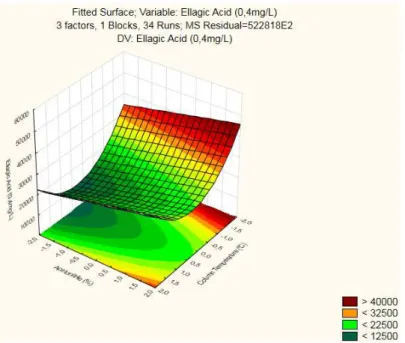
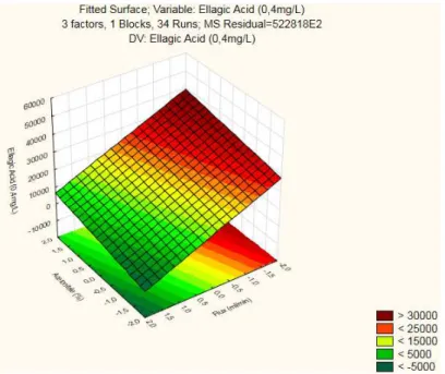
Figure 3. 3 - RSM for Ellagic Acid (0,4mg/L): Flux x Column Temperature
Figure 3. 4 - Contour Plot for Ellagic Acid (0,4mg/L): Flux x Column Temperature
34
Figure 3. 5 - RSM for Ellagic Acid (0,4mg/L): Flux x Acetonitrile
Figure 3. 6 - Contour Plot for Ellagic Acid (0,4mg/L): Flux x Acetonitrile
35
Summarizing, it’s the interaction Flux x Column Temperature that attains the highest peak area (>50000) for both factors low levels, presenting a Response Surface with curvature. This interaction is aligned with the significant factors found in the Reduced ANOVA (Table 3.5).
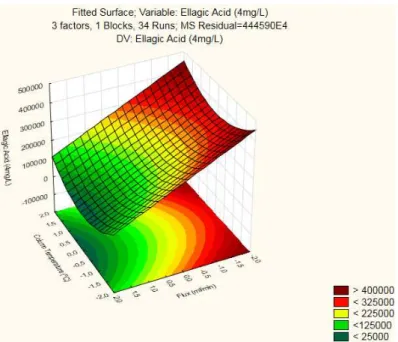
Ellagic Acid (4 mg/L)
For studying the curvature produced by this standard, RSM and Contour Plots were produced for the 3 factor interactions and can be found in the Appendixes.
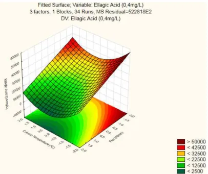
From the three Response Surfaces produced, it was the interaction between Flux and Column Temperature that yielded the highest peak (>400000), which was obtained for a low Flux . This surface also has a strong curvature component as it was expected given that its Reduced ANOVA (Table 3.13) found the two Quadratic components to be significant.
36
Figure 3. 8 - Contour Plot for Ellagic Acid (4mg/L): Flux × Column Temperature
3.1.4.
Regression Model
Ellagic Acid (0,4mg/L)
For building the Regression Model’s equation, are needed the coefficients which can be extracted from Table 3.7.
Table 3. 7 – Regression Coefficients for 0,4mg/L Ellagic Acid
Regress. Coeff. Std.Err. t(29) p -95,% +95,%
Mean/Interc. 17192,13 1683,015 10,21508 0,000000 13750,0 20634,28
Column Temp. (ºC)(L) -2927,88 1383,516 -2,11626 0,043027 -5757,5 -98,27
Column Temp. (ºC)(Q) 4259,45 1416,460 3,00711 0,005402 1362,5 7156,43
Acetonitrile (%)(L) 2859,00 1383,516 2,06648 0,047816 29,4 5688,61
Flux (ml/min)(L) -8253,36 1383,516 -5,96550 0,000002 -11083,0 -5423,75
The generic form of the Regression Model is presented by the following equation:
𝑌 = 𝛽0+ ∑ 𝛽𝑖 𝑘
𝑖=1
𝑋𝑖+ ∑ 𝛽𝑖𝑖 𝑘
𝑖=1
𝑋𝑖2+ ∑ ∑ 𝛽𝑖𝑗 𝑘
𝑗
𝑋𝑖𝑋𝑗 𝑘−1
𝑖
+ 𝜀
By replacing βx for the respective coefficients that can be extracted from this table’s second row, it’s possible to obtain the regression equation:
37
Assumptions that are assumed for the mathematical model and respective Analysis of Variance need to be validated, which is done by verifying if residuals are independent, normally distributed, with a null average and constant variance. Residuals are obtained from the difference between observed values and predicted/estimated values.
Normality verification is made by plotting a Normal probability distribution graphic, and if the results are disposed approximately according to a straight line it’s possible to conclude that the Normality assumption is satisfied. So, through an observation of residuals exposed in Figure 3.9 it’s possible to confirm that the assumption is verified.
Figure 3. 9 - Normal Probability Plot of Residuals for Ellagic Acid (0,4mg/L)
38
Figure 3. 10 - Predicted vs. Residual Values Plot for Ellagic Acid (0,4mg/L)
By plotting the Residuals vs. Case Numbers it’s possible to evaluate the independence of residuals. Its independence is proven if they’re randomly distributed in the graphic, such as they’re in Figure 3.11.
39
Ellagic Acid (4mg/L)
From the Regression Coefficients Table that can be found in the Appendixes was built the following Regression Model for Ellagic Acid (4mg/L):
𝑌 = 170867,3 − 85552,5𝑥3+ 27881,4𝑥12− 29423,1𝑥22
Analysis of Residuals for this compound proving that the data is normal, independent and its variance is constant can be found in the Appendixes.
Ferulic Acid
3.2.1.
Experimental plan
The responses in Table 3.8 show the values resultant from applying the variation of conditions planned to Ferulic Acid samples, for 0,2mg/L and 2mg/L standards. By observing results, it’s possible to see that the 1st experiment achieved the highest response (45016 and 44441) for the low concentration standard, while for the high concentration standard (240727 and 241335) it was the 3rd experiment. For this compound, it’s possible to verify that low levels of Temperature and Flux are yielding the best results, while the Solvent Concentration (% of Acetonitrile) varied between low and high levels.
Table 3. 8 - Experimental plan and respective responses for Ferulic Acid solution
Responses
Factors 0,2 mg/L 2 mg/L
Std.
Order
A B C 1st
Injection 2nd Injection 1st Injection 2nd Injection
1 34 21 0,25 25417 25072 240727 241335
2 46 21 0,25 26785 27430 240457 240791
3 34 79 0,25 45016 44441 203279 185410
4 46 79 0,25 30256 30284 109443 112743
5 34 21 0,40 15348 17301 145846 147574
6 46 21 0,40 15300 15681 145898 145751
7 34 79 0,40 18123 17157 56828 42677
8 46 79 0,40 18033 17826 55990 60441
9 40 50 0,33 23606 23198 128176 112903
10 40 50 0,33 21602 21478 122661 122255
11 40 50 0,33 16920 16860 38539 48236
12 50 50 0,33 19839 21178 182354 180875
13 30 50 0,33 14832 14584 89853 90206
14 40 99 0,33 33996 32993 192302 192700
15 40 1 0,33 20924 19985 113945 119009
16 40 50 0,45 21711 21868 121234 116627
40
3.2.2.
Analysis of Variance
Ferulic Acid (0,2mg/L)
The ANOVA performed for this compound can be found in the Appendixes. By inserting the variance of non-significant factors into the error’s variance, a Reduced ANOVA was achieved (Table 3.9). Regarding these results, it’s possible to observe that there are 5 significant components: Acetonitrile (L), Flux (L), Flux (Q), Column Temperature x Acetonitrile, Acetonitrile x Flux. Although, it’s the Flux’s linear component that presents a lower p-value and consequently has more influence in system’s response.
Table 3. 9 - Reduced ANOVA for 0,2mg/L Ferulic Acid
Var.: Ferulic Acid (0,2 mg/L)
SS df MS F p
Acetonitrile (%) (L) 6,044061E+07 1 6,044061E+07 4,53134 0,042553
Flux (ml/min) (L) 1,227722E+09 1 1,227722E+09 92,04462 0,000000
Flux (ml/min) (Q) 5,976066E+07 1 5,976066E+07 4,48037 0,043647
1L by 2L 5,774480E+07 1 5,774480E+07 4,32924 0,047079
1L by 3L 3,630665E+07 1 3,630665E+07 2,72198 0,110563
2L by 3L 8,922692E+07 1 8,922692E+07 6,68951 0,015411
Error 3,601351E+08 27 1,333834E+07
Total SS 1,891337E+09 33
Through an analysis of the coefficient of determination, R2= 0,80959, we can verify that for Ferulic Acid (0,2mg/L) the regression model approximates the real data.
Ferulic Acid (2mg/L)