Topologies Induced by Relations with Applications

ISSN 1549-3636

© 2008 Science Publications

877

Topologies Induced by Relations with Applications

A.S. Salama

Department of Mathematics, Faculty of Science, Tanta University, Egypt

Abstract: Topological structures induced by relations represents the process of extracting interesting decision rules from data. The attributes reduction and the calculation of core are the essentials to extract the decision rules. Finding the reducts, core and decision rules topologically is a new mathematical tool for discovering attribute dependencies in information systems. Problem statement:

These mathematical tools employ some concepts from topological spaces, relational databases, rough sets and information systems. The results using our approach are more accurate and applicable than that using the classical approaches such as in the father's approach of rough sets (Pawlak approach).

Approach: Topologies generated using dominance (pre-order) relations and general binary relation are the knowledgebase of our approximations. We suggested a new algorithm (openness algorithm ) based on the topologies induced by general relations. Results: Results obtained by the proposed approach to find the reducts and core in terms of open and closed sets are compared with the existing method. Our proposed method is proved to be the accurate than results of any approaches using some types of binary relations such as order(pre-order) relations or symmetric relations. Conclusion: In this study, There are many approaches for obtaining topologies by relations and we used some of them in data reduction. These approaches were generalizations to Pawlak approaches namely, we ignored the notion of equivalence relations. Also, these approaches open the way for other approximations if we use the general topological recent concepts such as pre-open sets or semi-open sets.

Key words: Topological spaces, binary relations, relational databases, information system, rough sets, data reduction

INTRODUCTION

Topology is an important and interesting area of mathematics, the study of which will not only introduce you to new concepts and theorems but also put into context old ones like continuous functions. It is so fundamental that its influence is evident in almost every other branch of mathematics. This makes the study of topology relevant to all who aspire to be mathematicians whether their first love is algebra, analysis, category theory, chaos, continuum mechanics, dynamics, geometry, industrial mathematics, mathematical biology, mathematical economics, mathematical finance, mathematical modeling, mathematical physics, mathematics of communication, number theory, numerical mathematics, operation research or statistics. Topological notions like compactness, connectedness and denseness are as basic to mathematicians of today as sets and functions were to those of last century[3,8,9].

For a long time, many individuals believed that abstract topological structures have limited application in the generalization of real line and complex plane or some connections to Algebra and other branches of

mathematics. And it seems that there is a big gap between these structures and real life applications. We noticed that in some situations, the concept of relation is used to get topologies that are used in important applications such as computing topologies[15], recombination spaces[2,7,16] and information granulation which are used in biological sciences and some other fields of applications.

The aim of rough set theory is to give a description of the set of objects by logical, set-theoretical, topological etc. tools in terms of similarity relations and derived notions related by these relations. The description of the set of objects entails as well relationships and functional or near to functional dependencies among various similarity relations generated by various sets of the set of objects.

MATERIALS AND METHODS

878 Furthermore, we assume Ob to be finite. For x∈Ob, let [x]R be the equivalence class containing x, i.e.,

[x]R = {y: y R x }.

Given an arbitrary set X⊆Ob, we wish to describe X in terms of elements or granules of Ob/R. Pawlak proposed the use of lower and upper approximations of a set X, denoted R(X) and R (X), respectively. Lower and upper approximations are defined as:

R(X) = {x∈Ob:[x]R ⊆X}

R(X) = {x∈Ob: [x]R∩X ≠ φ}

The semantics of the approximations of sets may be defined as follows:

• Elements of the universe that belong to R (X) are those elements that surely belong to the set X • Elements that belong to R (X) possibly belong to

the set X

• Elements that belong to Ob/R (X) are elements of the universe that surely do not belong to the set X. Hence, the uncertainty lies in R (X)/ R (X) which is also called area of uncertainty. Elements of the area of uncertainty may, or may not, belong to X The approximation operators can also be considered using membership functions. It is possible to define a rough membership function as presented in[12].

Topologies induced by relations: Let A = (Ob, R) be an approximation space. The equivalence classes Ob\R of the relation R will be called elementary sets (atoms) in A. Every finite union of elementary sets in A will be called a composed set in A. The family of all composed sets in A will be denoted by com (A).

The family com (A) in the approximation space A = (Ob, R) is a topology on the set Ob.

Since the approximation space A = (Ob, R), defines uniquely the topological space τ (A) = (Ob, com (A)) and com (A) is the family of all open sets in τ (A) and U/R is a basis for τ (A), then τ (A) is a quasi-discrete topology on Ob and com (A) is both the set of all open and closed sets in τ (A). Thus, the lower approximation and the upper approximation of any subset X⊆Ob can be interpreted as the interior and the closure of the set X in the topological space τ (A), respectively.

Lemma 1: If β is a base for a topological space (Ob,τ),

where β is a partition of Ob, then for every subset X⊆Ob:

• int_τ(X)= {B∈β:B⊆X} • clτ(X)= {B∈β:B∩X≠ϕ}

Proof: Only we prove (ii) because (i) is trivial. Let x∈clτ (X) then for every open set G containing x, X∩G ≠ ϕ. But

B

G B,

∈β

= then there exists Bo ⊆G such

that x∈Bo⊆G. But Bois an open set containing x, hence

Bo∩X ≠ ϕ and x∈U{B∈β: B∩X ≠ ϕ}.

Conversely, if x∈ {B∈β:B∩X≠ϕ} and G is an open set containing x and β is a partition of Ob, x∈U_,

then x belongs to only one element of β say x∈Bo.

Then must Bo ⊆ G, i.e., x∈Bo⊆G but Bo∩X ≠ ϕ, hence

G∩X ≠ ϕ. Then x∈clτ(X).

Let A1 = (Ob, R1) and A2 = (Ob, R2) be two

approximation spaces. Then we say that the partition Ob/R depends on the partition Ob/R2 denoted Ob/R1 if

and only if

2

1 S Ob / R

B S, B Ob / R

∈

= ∀ ∈ .

Proposition 2: Let τ1 and τ2 be the topologies induced

by the partitions Ob/R1 and Ob/R2 respectively. Then

Ob/R1 Ob/R2 iff τ2⊆τ1.

Example: Consider the partitions β1 = {{x1, x2}, {x3},

{x4}} and β2 = {{x1, x2}, {x3, x4}} of the set Ob = {x1,

x2, x3, x4}. Then β1 β2 and τ2 ⊆ τ1 where τ1 = {Ob, φ,

{x3}, {x4}, {x1,2}, {x3, x4}, {x1, x2 x3}, {x1, x2 x4}},

τ2 = {Ob, φ, {x1, x2}, {x3, x4}} are the topologies

generated by β1 and β2 respectively.

For any topological space (Ob,τ), we define the equivalence relation E(τ) on the set Ob by

Ob y , x , }) y ({ cl }) x ({ cl iff ) ( E ) y , x

( ∈ τ τ = τ ∀ ∈ .The set of

all equivalence classes of E(τ) is denoted by Ob/ E(τ).

Proposition 3: Let A = (Ob, R) be an approximation space and let τR be the topology generated by the base

BR = Ob/R. If (Ob, τ) is the quasi-discrete topological

space has Ob/E(τ) as a base. Then τR = τ iff for all

x∈BR∈βR there exists B∈Ob/E(τ) such that x∈B. Lemma 4[15]: For any topology τ on a set Ob and for all x, y∈Ob, if y∈clτ({x}) and x∈clτ({y}) then clτ ({x}) = clτ ({y}).

Lemma 5[15]: If τ is a quasi-discrete topology on a set

Ob, then y∈clτ ({x}) implies x∈clτ ({y}) for all x, y∈Ob.

Lemma 6[15]: If τ is a quasi-discrete topology on a set

879

Proposition 7: Let τ be the topology induced by the partition βR = Ob/R . Then βR = Ob/E(τ).

Proof: x∈∈∈B, B∈β∈ R

• iff

y B

x cl (B)τ cl ({y})τ ∈

∈ =

• iff yo ∈ B and x∈clτ({yo}) iff clτ({x}) = clτ({yo})

(Lemma 2.2) • iff (x, yo) ∈ E(τ)

• iff A∈Ob/E(τ) such that x ∈ A • iff βR = Ob/E(τ)

For any n approximation spaces A1 = (Ob, R1),

A2 = (Ob, R2),…, An = (Ob, Rn) we define the partition

ind i

i 1,2,...,n

Ob / E( ) Ob / E( )

=

τ = τ .

Theorem 8: τi ⊆ τind, i = 1, 2,…, n where τi and τind are

the topologies generated by the partitions Ob/(τi) and

Ob/E(τind) respectively.

Proof: Since Ob/E(τind) ≤ Ob/E(τi) for all i = 1, 2,…, n

then τI ⊆ τind.

Example: Consider the topological space (Ob, τ) where

Ob = {x1, x2, x3, x4} and b = {{x1}, {x2, x3}, {x4}} is

the base of τ, then τ is a quasi-discrete topology and:

} x { }) x ({

clτ 1 = 1 ,clτ({x2})={x2,x3},clτ({x3})={x2,x3}

} x { }) x ({

cl_{τ 4} = ₄

Then Ob/E(τ) = {{x1}, {x2, x3}, {x4}} = β.

Example: Consider the approximation spaces

1 1

A =(Ob, R ), A2=(Ob,R2) and A3=(Ob,R3) where

} x , x , x , x {

Ob= 1 2 3 4 and Ob/E(τ1) = {{x1}, {x2, x3},

{x4}}, Ob/E(τ2) = {{x1, x2}, {x3, x4}} and Ob/E

(τ3) = {{x1}, {x2}, {x3, x4}}are the bases of τ1, τ2 and τ3

respectively, then Ob / E(τind)=(Ob / E( ))τ1 ∩(Ob / E( ))τ2

3 1 2 3 4

(Ob / E( )) {{x },{x },{x },{x }}

∩ τ = is the partition

induced by E(τind). Then τι ⊂ τind, i = 1, 2, 3.

Topologies generated using similarity relations: A similar relation R on Ob is any relation satisfies: • For any x∈Ob, xRx (reflexive)

• For any x, y∈Ob, if xRy then yRx (Symmetric) For x∈Ob, we define the similar class containing x by R(x)= {y∈Ob: xRy}.

The relation R on Ob defined by xRy iff d(x,y)<n where (Ob, d) is a metric space with a metric function d defined as: d(x,y) = x−y and n = card (Ob), is a similar relation.

Proposition 9 For any similar relation R defined on Ob we have:

• x∈R(x)

• y∈R(x) iff x∈R(y)

• xRy iff x∈R(y) and y∈R(x)

The class = {B(x): x∈X} is called a symmetric covering of a set X if x∈B(y) iff y∈B(x). Then the class = {R(x): x∈Ob} is a symmetric covering of the set of objects Ob.

Let is the symmetric covering of Ob by the similar relation R. Then we define a relation R induced by by x R y iff there exist B∈ and x,y∈B.

Proposition 10: The relation R is a similar relation on the set of objects Ob.

Since β is a covering of Ob, then for any x∈Ob there exists B∈β such that x∈B hence x, x∈B∈β then xR x. Let xR y then there exists B∈ such that x, y ∈B then y, x∈B hence yR x.

Proposition 10 for every x∈Ob we have:

R (x) =

) ( B

B

x

β ∈

, where β(x) = {B∈β: x∈B}

Proof:

y∈Rβ(x) ⇔ ∃ B∈ β and x,y∈B ⇔ ∃ B∈ β and x∈B and y∈B ⇔ ∃ B∈ β and y∈B

⇔

B ( x )

B

∈β

Let is the covering of Ob. Then we define the class β* = {R (x): x∈Ob}.

Proposition 11: The class * is a symmetric covering of the set of objects Ob and R ⊆ R*.

Proof:

• x∈Rβ(y) ⇔ ∃ B∈β(y) and x∈B ⇔∃ B∈β(x) and y∈B ⇔ y∈Rβ(x)

• Let (x,y) ∈ Rβ ∃ B∈β and x, y ∈B B∈ β(x) and B∈ β(y)

880 B∈

B ( x )

B

∈β = Rβ(x)∈β*

x,y∈B∈β* x,y∈Rβ*

Let A⊆Ob be any non empty subset of the set of objects. Then A is called a similar pre-class of R if for any x,y∈A (x,y)∈R.

Proposition 12 Every similar class R(x) is a maximal similar pre-class.

For an element x∈Ob we define a class called the pre-similar class of x as follows:

LR(x) = {A⊆Ob: x∈A and A is similar pre-class of R}.

Let LR = {LR(x): x∈Ob} be the family of all pre-similar

classes. Then we define a relation R* on LR by for any

LR(x), LR(y) ∈ LR, LR(x)R*LR(y) iff there exist

A∈LR(x) and B∈LR(y) and A B ≠ϕ.

Proposition 13:

• The relation R* on LR is a similar relation

• xRy iff LR(x)R*LR(y) for any x,y∈Ob Proof:

• Since for any LR(x) ∈ LR and A∈LR(x), A A ≠ φ

then LR(x)R*LR(x) hence R* is reflexive. Also if

LR(x)R*LR(y) then there exist A∈LR(x) and

B∈LR(y) such that A B ≠ φ, hence B A ≠ φ,

hence LR(y)R*LR(x). Then R* is symmetric

• Firstly, we will prove that xRy LR(x)R*LR(y)

Let (x, y)∈R {x, y}is a similar pre-class of R. there exist a similar class R(x) such that {x,y}⊆ R(x) and R(x)∈LR(x) but R is symmetric then

R(x)∈LR(y), then there exist A = R(x)∈LR(x) and

B = R(x)∈LR(y) and A B ≠ ϕ, hence LR(x)R*LR(y).

Conversely, let for some x,y∈Ob, LR(x)R*LR(y)

then there exist R(z)∈LR(x) and R(z)∈LR(y) a similar

class of R. hence x∈R(z) and y∈R(z) then x,y ∈R(z) hence xRy.

Let LR (x) be the pre-similar class of x∈Ob. Then

we define a set L*

R(x) =

R

A L ( )

A

∈ x

called the R-link of x, where A∈L

R(x) and A ≠ R(x).

If L*R(x) = Ob then it is called open R- link of x

and if L*R(x) ⊂ Ob then it is called closed R- link of x.

The class M={ L*R(x): x∈Ob} of all R- links of

x∈Ob is a subbase of a topology on Ob called the linked topology and denoted τL*_R.

Proposition 14:

• For any x∈Ob, L*

R(x) ⊆ R(x)

• The class M is a symmetric covering of Ob

Proof:

• Let y∈L*R(x) y∈

R

A L (x )

A

∈ there exists

A = R(x)∈LR(x) and y∈A then y∈R(x) L*R(x) ⊆ R(x)

• For any x∈Ob, x∈L*

R(y) M is covering of Ob

Now let x∈ L*

R (y) x∈

R

A L (x )

A

∈ :

• there exist A=R(x) ∈ LR(y) and x∈R(x)

• x, y ∈R(x) • y∈ L*

R (x)

then M is a symmetric covering of Ob.

Proposition 15:

• The linked topology τL*_Ris finer than the similar

topology R, where R is the topology generated by

the subbase {R(x): x∈Ob}

• xRy ∃ open set u∈τL*_Rand x,y∈u

Example: Let Ob = {c1,c2,…, c7} be the set of objects

which is seven computers in a local network in a certain company. Let be the irregular topology on the set of objects which induced by a general relation on Ob which makes the following graph. We define a similar relation R on the set of objects by: Two computers x and y are in relation by R iff the computer x has a copy of a certain program in the computer y.

Then we can define the similar classes of R as follows:

• R(c1) = {c1, c2, c4}, R(c2) = {c1, c2, c3,c4, c5}, R(c3)

= {c2, c3, c5}, R(c4) = {c1, c2, c5, c6, c4}, R(c5) = {c2,

c3, c4, c6, c5}, R(c6) = {c4, c5, c6, c7}, R(c7) = {c6,

c7}. Then we have LR(c1) = {{c1}, {c1, c2}, {c1, c4},

{c1, c2, c4}}, LR(c2) = {{ c2}, {c2, c1}, {c2, c4}, {c2,

c5}, {c2, c3}, {c2, c3, c5}, {c2, c1, c4}, {c2, c4, c5},

{c2, c1, c3, c4, c5}}, LR(c3) = {{c3}, {c3, c2}, {c3,

c5}, {c3, c2, c5}}, LR(c4) = {{c4, {c4, c1}, {c4, c2},

{c4, c5}, {c4, c6}, {c4, c1, c2}, {c4, c2, c5}, {c4, c5,

c6}, {c4, c1, c2, c5, c6}}, LR(c5) = {{c5}, {c5, c2},

{c5, c4}, {c5, c3}, {c5, c6}, {c5, c2, c3}, {c5, c2, c4},

881 c4}, {c6, c5}, {c6, c7}, {c6, c4, c7}, {c6, c5, c7}, {c6,

c4, c5}, {c4, c5, c6, c7}}

• LR(c7) = {{c7}, {c6, c7}}. Also, we have:

L*R(c1) = {c1, c2, c4}, L*R(c2) = {c1, c2, c3, c4, c5},

L*R(c3) = {c2, c3, c5} L*R(c4) = {c1, c2, c5, c6, c4},

L*R(c5) = {c2, c3, c4, c5, c6}, L*R(c6) = {c4, c5, c6,

c7}, L*R(c7) = {c7}

Then the linked topology τL*_R is finer than the

similar topology, such that L*R(ci) ⊆ R(ci) for all

i = 1,2,…,7.

For any subset A of the set of objects, we define two sets R(A) and R(A), they are called the lower and upper similar classes of A by:

R(A)= {R( ) : R(x)x ⊆A}

and

} A ) ( R : ) ( R { ) A (

R = x x ≠ϕ

Let τR be the topology induced by the subbase

{R(A) : A⊆Ob}this topology called the lower similar topology. Also we define the topology τR which is

called the upper similar topology and generated by the subbase {R(A) : A⊆Ob}.

Proposition 16: Let τ_R and τRbe the lower and upper

similar topologies then:

• τR⊆τR if R is an equivalence relation

• τR⊆τ_Rif R is a similar relation

• τR and τRare in general not comparable if R is a

general relation

The following proposition present another way to generate topologies from similarity relations.

Proposition 17: τ**R={A⊆Ob:∀x∈A,R(x)⊆A} is a topology on Ob.

Proof:

• Ob,ϕ∈τ**R is clearly

• If A1, A2, … ∈ τ**R and i i

x∈ A for some i then

i

R(x)⊆A then

i i

A )

R(x ⊆ hence **

i R i

A ∈ τ

• Let A1, A2 ∈ τ**R , then ∀x∈A1 A2 we have 1

R(x)⊆A and R(x)⊆A2 hence R(x)⊆A1 A2

then **

1 2 R

A A ∈ τ

Example: Consider Ob = {a, b, c, d} be the set of objects with a similar relation R its similar classes are: • R(a) = {a, c}, R(b) = {b, d}, R(c) = {a, c, d} and

R(d) = {b, c, d}. Then: τR = {Ob, ϕ {c}, {d}, {c,

d}, {a, c}, {b, d}, {a, c, d}, {b, c, d}}, τR= {Ob, ϕ,

{d, c}, {a, c, d}, {b, c, d}} and τ**_{R = {Ob, ϕ} then}

τ**

R ⊂ τ ⊂ τR R

• The conjugate relation R of R is defined by (x, y) ∈ R iff (x, y) ∉ R or x = y

Proposition 18:

• R R=I, I is the identity relation • Ris a similar relation

• R=R

Proof:

• (x, y)∈R R iff x = y R R=I

• (x, x)∈R such that x = x and if (x, y)∈R then (x,y)∉R or x = y then (y,x)∉R or y = x hence (y,x)∈R

• (x, y)∈R ⇔( x,y) ∉ R or x = y ⇔ (x,y)∈R or x = y ⇔(x,y)∈R

Example: Let Ob = {a, b, c, d} be the set of objects with the similar relation R = {(a, a), (b, b), (c, c), (d, d), (d, c), (c, d), (d, b), (b, d), (c, b), (b, c), (b, a), (a, b)}. Then R=I (Ob×Ob−R) = {(a,a), (b,b), (c,), (d,d), (c,a), (a,c), (d,a), (a,d)}.

Topologies generated using dominance (pre-order) relations: For a long time, many mathematicians believed that there is a large deviation between abstract topological structures and computing[12-14].

A relation R on a set Ob is called a dominance relation (pre-order) whenever R is both reflexive and transitive . If x is related to y, we write xRy and say that x dominances y. The set R(y)={x:yRx} is called the before set.

Example: Let Ob=

{

}

R = {(1, 1), (1, 2), (1, 3), (1, 4), (1, 5), (4, 4), (5, 5), (6, 6), (1,6), (2, 2), (2, 4), (2, 6), (3, 3), (3, 6)}. The relation R is a dominance relation.

In a finite space ( Ob, ),τ it is clear that }

G : G Ob {

c_{= − ∈τ}

882 A subset F⊂X is a closed set iff F Fy

F y∈

= such

that Fy={x:yRx} (Fy is the smallest closed set about x). This is the dual of our representation of open sets.

If R is a dominance relation on a set Ob, then its dual RD is defined by the requirement yRD x if and

only if xRy.

A point x in a subset U of Ob is insulated from U

Ob− if and only if there is no point y in Ob−U such that y dominates x.

Lemma 19: Let R be a dominance relation on a set U

P , Ob U ,

Ob ⊂ ∈ the following are equivalent s: • P is insulated from Ob−U

• P∈U,(y,P)∈R, then y∈U

Proof: First, consider p∈U is insulated from Ob-U, (y,

p) ∈R. Let y∉U, then y∈Ob-U, So (y, p)∉R, but (y, p)∈R, a contradiction, then y∈U.

Second, consider p∈U, x ∈Ob-U, suppose (x, p) ∈R. Then x∈U contradicts that x∉U, then τR={U

} U x , U b O from insulated is

x :

Ob − ∀ ∈

⊂ (x, p)∉R.

Proposition 20: If R is a dominance relation on a set Ob, then is topology on Ob.

Proof: Clearly Ob and φ are elements in τR let Ui∈ τR

for every i∈I. For any i I i

U x

∈

∈ and (y, x)∈R, there is i0∈I such that x∈U .i0 By openness of U ,i0 we have

i I i

i U

U y

0 ⊂ ₌

∈ . Therefore i R

I i

U ∈τ

∈ . Also, if A and B

are elements of τR, then {Ob, ,{d}} 2

ϕ = τ−

− .

According to the above proposition we give the following algorithm to check the openness of a subset

Ob

U⊂ with respect to a dominance relation R.

Openness algorithm:

i- Find Ob-U

ii- Investigates the existence of any pair (a, b) U

b , U Ob a ,

R ∈ − ∈

∈ , we have two cases:

• If there exists such pair, then U is not open

• If there is not such pair (a, b), then U is open

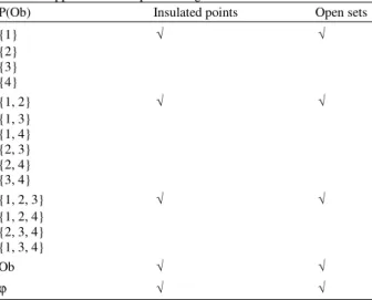
The following example (Table 1) is an application for the above algorithm.

Table 1: Application for Openness algorithm

P(Ob) Insulated points Open sets

{1} √ √

{2} {3} {4}

{1, 2} √ √

{1, 3} {1, 4} {2, 3} {2, 4} {3, 4}

{1, 2, 3} √ √

{1, 2, 4} {2, 3, 4} {1, 3, 4}

Ob √ √

ϕ √ √

Then the induced topology is τR = {Ob, ϕ, {1}, {1,

2}, {1, 2, 3}}.

Let Ob be the set of objects and let R be any binary relation on Ob. The relation R gives rise to a closure operator clR as follows:

clR(A) = AU{y∈X}|∃x∈A: (y, x)∈R} for every A⊆Ob Lemma 21: The interior operator corresponding to clR

is given by:

intR(A) = {y∈A: ∀x∈Ac, ∼yRx} Proof: intR(A) = [clR(Ac)]c

= {Ac {y∈X: ∃x∈Ac, (y, x)∈R}}c = A {y∈X: ∃x∈Ac, (y, x)∈}c = A {y∈X: ∀x∈Ac, (y, x)∉R}c = {y∈A: ∀x∈Ac_{, ∼yRx}}

Thus the interior operator of A consist of those elements of A which are not R-related to any elements outside A.

Lemma 22: For any relation R on Ob , (Ob,clR)is closure space.

In the following we will give an example (Table 2) for closure space generated by a general relation.

Example: Consider Ob{a, b, c} and R is a binary relation on Ob, R = {(a, b), (c, b), (a, c)}. Then we have the Table 2 for closures and interiors of the subsets of Ob: We note from Table 2 that:

• clR(φ) = φ

• A ⊆ clR (A)

883

Table 2: Closure space generated by a general relation

A ClR (A) intr (A)

{a} {a} φ

{b} {b, c} {b}

{c} {a, c} φ

{a, b} Ob {b}

{a, c} {a, c} φ

{b, c} Ob {b, c}

Ob Ob Ob

φ φ φ

Table 3: Closures and interiors of the subsets of Ob

A ClR (A) intR (A)

{1} {1} {1}

{2} {2, 3} φ

{3} {2, 3} φ

{1, 2} Ob {1}

{1, 3} Ob {1}

{2, 3} {2, 3} {2, 3}

Ob Ob Ob

φ φ φ

Lemma 23 If Ob be non-empty set and R is transitive relation, then (x, clR) is topological space.

Example: Consider the relation R = {(1, 1), (2, 3), (3, 2), (2, 2)} on Ob = {1, 2, 3}. Table 3 shows closures and interiors of the subsets of Ob.

From Table 3, we have: • clR(φ) = φ

• A⊆clR(A

• clR(A B) = clR(A) clR(B) for all A, B ⊆ Ob

• clR(clR(A)) = clR(A) for all A ⊆ Ob

Topologies generated using general binary relations:

The basic aim of this section is to generate topological structures using the lower and the upper approximations of any binary relation. Given general approximation space A=(Ob,R)where R here is any general binary relation on Ob. For any subset X of Ob we define lower and upper approximations as follows:

)} X y R ) y , x (( y : Ob x { ) X (

R = ∈ ∀ ∈ ∈

− and )} X y R ) y , x (( y : Ob x { ) X (

R = ∈ ∃ ∈ ∧ ∈

−

Then the following structures are topologies on Ob: } G ) G ( R : Ob G {

1= ⊆ =

τ − − } G )) G ( R ( R ) G ( R : Ob G { 2 2 = = ⊆ = τ − − − − } G ))) G ( R ( R ( R ) G ( R : Ob G { 3

3= ⊆ = =

τ − − − − − ….. } Ob n , G ) G ( R : Ob G

{ n1

1 n = = ⊆ = τ − − − −

These topologies have the property that:

1 − τ ⊆ 1 n 2 .... − −

− ⊆ ⊆τ

τ .

Also, if we deal with the upper approximation instead of the lower approximation we can construct the following topologies: } ) G ( R G ) G ( R : Ob G {

1= ⊆ = ∨ =ϕ

τ− − −

2

2 {G Ob : R (G) R(R(G)) G R(R(G)) }

− − − − − −

τ = ⊆ = = ∨ = φ

3

3 {G Ob : R (G) R (R (R (G))) G R (R (R (G))) }...

− − − − − − − −

τ = ⊆ = = ∨ = φ

n 1 n 1

n 1 {G Ob : R (G) G R (G) , n Ob }

− −

− − −

−

τ = ⊆ = ∨ = φ =

These topologies have the property that

1 n 2

1 .... − − − − τ ⊆ ⊆ τ ⊆ τ .

In the following we will give some illustrative examples and remarks.

Example: Let Ob={a,b,c,d}be the universe and let )} b , c ( ), a , d ( ), d , b ( ), d , c ( ), b , a {(

R= be a general binary

relation on Ob. Then we have the following topologies on Ob using the lower approximation:

}} d , b , a { , , Ob { 1 ϕ = τ − }} d , b , a { , , Ob { 2 ϕ = τ − 3

{Ob, ,{a},{b},{d},{a, b},{a, d},{b, d},{a, b,d}}

−

τ = φ

If we made more iteration to introduce more topologies using the lower approximation we will obtain that:

1 4 −

− =τ

τ ,

2 5 −

− =τ

τ and

3 6 −

− =τ

τ and so on. Also we have the following topologies on Ob using the upper approximation:

}} c { , , Ob {

1= ϕ τ− }} c { , , Ob {

2= ϕ τ−

3 {Ob, ,{d},{c},{a,c},{b,c},{a, b,c},{a,c,d},{b, c,d}}

−

τ = φ

If we made more iteration to introduce more topologies using the upper approximation we will obtain that: τ4=τ1, τ5=τ2 and τ6=τ3 and so on.

Remark: If the relation R on the universe Ob is constant, then all topologies induced by the lower or the upper approximations are indiscrete.

884 If we made more iteration to introduce more topologies using the lower approximation or the upper approximation, then all new iterations will introduce the same topologies we before obtained.

Another method for constructing topologies using the lower and the upper approximations is presented bellow:

All the following are topologies on Ob:

)} G ( R ) G ( R : ) G ( R { 1 ₋ − − − − = = τ )} G ( R ) G ( R : ) G ( R { 2 2 2 2 ₋ − − − − = = τ )} G ( R ) G ( R : ) G ( R { 3 3 3 3 ₋ − − − − = = τ

……, {R (G):R (G) R (G)}

1 n 1 n 1 n 1

n − −

− − − − − − − = = τ

Also, all the following structures are topologies on Ob. 1

{R(R(G)) : R(R(G)) R(R(G))},

− − −

− − −

τ = = −

−

= τ2 {R(R

)))} G ( R ( R ( R ))) G ( R ( R ( R : ))) G ( R ( − − − − − −

− = and so on.

Example: According to Example we have:

}} c , b , a { }, d { , , Ob { 1 ϕ = τ − − }} d { , , Ob { 2 ϕ = τ − − }} d { , , Ob { 3 ϕ = τ − − RESULTS

The basic aim of our paper is to generate topological structures that are used to generate many topological measures and then using it in data reduction. First, we are used general binary relation to generate topological structures using the lower and the upper approximations. Make use of these methods we succeeded to introduce many topologies such as lower topologies from degree 1 to degree n where n is any order. Also, the topologies from degree 1 to n using upper approximations. Second, we are used the approach of closure operator and interior operator to induced topological structures.

We govern the importance of these topologies by the specified properties of relations that it are generate. Lemmas, propositions and theorems are mentioned to filter these topology to know which topology is used in applications of data reduction.

Table 4: The information system

Ob a1 a2 a3 a4

x1 1 2 9 6

x2 3 2 6 2

x3 3 6 3 3

x4 4 2 2 3

x5 6 6 5 4

In our application example we succeeded to obtain reducts of multi-valued (set-valued) datasets that handled differently using ROSETTA software and proved that our solution is more accurate than solution in[10,14].

Now if τI_At is the topology induced by

} Ob X : ) X ( Int

{ _At ⊆ (τC_Ator τNAtcan be used alternately),

then when τi,j=τI_At the set {ai,aj}is a second order

reduct of At in S. On the other hand, if τi,j≠τI_Atfor all i,

j = 1,2,…,n we must calculate the highest topologies

3 , 2 , 1

τ ,…, τn−2,n−1,n and the subset {ai,aj,ak} is a third

order reduct of At in S when τi,j,k=τI_AT. By the same

manner, we can define a highly order reducts of At in S. In each case, the topological core of At in S is the intersection of all reducts (intersection of all the same order reducts). This core called the interior core and denoted CoreInt (At). By the same terminology, we can

define the closure core (CoreC1 (At)) and the

neighborhood core (CoreN(At)).

Illustrated Example Consider the information system shown by Table 4 and if we choose r = 2, then

} 2 ) y ( f ) x ( f : Ob y { ) r , x (

Na_i = ∈ a_i − a_i ≤ , hence we have the

following subbases:

ς1 = {{x1, x2, x3}, {x1, x2, x3, x4}, {x2, x3, x4,x5}, {x4,

x5}}

ς2 = {{x1,x2,x4}, {x3,x5}}

ς3 = {{x1}, {x3, x4, x5}, {x2, x5}, {x3, x4}, {x2, x3, x5}}

ς4 = {{x2, x3, x4, x5}, {x1, x5}, Ob}

The corresponding bases are:

β1 = {{x1, x2, x3}, {x1, x2, x3, x4}, {x2, x3, x4, x5}, {x4,

x5}}, {x4}, {x2, x3}, {x2, x3, x4}}

β2 = {{x1, x2, x4}, {x3, x5}}

β3 = {{x1}, {x3, x4, x5}, {x2, x5}, {x3, x4}, {x2, x3, x5},

{x5}, {x3}, {x3, x5}}

β4 = {{x2, x3, x4, x5}, {x1, x5}, {x5},Ob}

The corresponding topologies are:

τ1 = {Ob, ϕ, {x1, x2, x3}, {x1, x2, x3, x4}, {x2, x3, x4, x5},

{x4, x5}, {x4}, {x2, x3}, {x2, x3, x4}}

885 τ3 = {Ob, ϕ, {x1}, {x3, x4, x5}, {x2, x5}, {x3, x4}, {x2,

x3, x5}, {x5}, {x3}, {x3, x5},{x1, x2, x5},{x1, x3, x4,

x5},{x1, x2, x3, x5},{x1, x3, x4}, {x1, x5}, {x1, x3,

x5},{x1, x3},{x2, x3, x4, x5},{x2, x3, x5}, {x3, x4,

x5}}

τ4 = {Ob, ϕ, {x2, x3, x4, x5}, {x1, x5}, {x5}}

If we considered the set of all attributes then τN_Atis

the discrete topology, but the second order topologies are given such that:τ1,2 ≠ τNAt,τ1,3= τNAt, τ1,4 ≠ τNAt,

2,3

τ = τNAt,τ2,4≠ τNAt,τ ≠3,4 τNAtThen {a1, a3} and {a2,

a3} are second order reducts of At and the second order

core is given byCore (At)N ={a }3 .

DISCUSSION

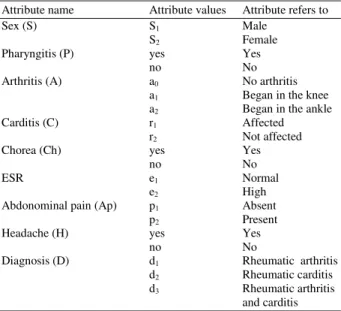
In this section, we briefly describe the main idea of our work using the rheumatic fever datasets. No doubt that, the rheumatic fever is a very common disease. It has many symptoms differs from patient to another but though the diagnosis it is the same. So, we obtained the following data on seven rheumatic fever patients from Banha fever hospital, Egypt. All patients are between 9-12 years old with history of Arthurian began from age 3-5 years. This disease has many symptoms and it is usually started in young age and still with the patient along his life. Table 5 introduced the seven patients characterized by 8 symptoms (Attributes) using them to decide the diagnosis for each patient (Decision Attribute). Table 6 shows the rheumatic fever information system.

Table 5: Rheumatic fever data

Attribute name Attribute values Attribute refers to

Sex (S) S1 Male

S2 Female

Pharyngitis (P) yes Yes

no No

Arthritis (A) a0 No arthritis

a1 Began in the knee

a2 Began in the ankle

Carditis (C) r1 Affected

r2 Not affected

Chorea (Ch) yes Yes

no No

ESR e1 Normal

e2 High

Abdonominal pain (Ap) p1 Absent

p2 Present

Headache (H) yes Yes

no No

Diagnosis (D) d1 Rheumatic arthritis

d2 Rheumatic carditis

d3 Rheumatic arthritis

and carditis

Let us consider the topological space τa generated

using binary relation defined on the attribute a. Also, using the same terminology the topological space τB is

the topology generated using general relation defined on a subset of attributes B of all condition attributes At. The decision attribute generates the topology τD.

Now, we will use the following suggestion, The set of attributes B⊆At is called a reduct if

D B ≤τ

τ and B is minimal, where:

) U ' G , G , ' G G . t . s ' G , G iff

(τB ≤τD ∀ ∈τB ∃ ∈τD ⊂ ≠

The attribute a∈At is called the core if a

b , At b , a ,

b

a τ ∀ ∈ ≠

τ .

When the classical technique of rough set theory (ROSETTA software)[4,5,13] used to obtain reducts and core of our data we found that we have 8 reducts of Table 6 with out any intersections among them. So, we do not have any core of Table 6. The set of obtained reducts is as follows:

}} H Ap A P { }, H C A {

}, Ap ESR A P { , } ESR C {

}, Ap K C A P { }, Ap A P S {

}, C A S { }, Ch C S {{ ) At ( d Re

∨ ∨ ∨ ∨ ∨

∨ ∨ ∨ ∨

∨ ∨ ∨ ∨ ∨

∨ ∨

∨ ∨ ∨ ∨ =

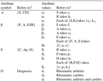
Now, after getting the reducts of Table6 using the ROSETTA software. We will convert Table5-8 using Table7.

Now we will apply the above contributions on Table 7 where Ob={x1,x2,x3,x4,x5,x6,x7} is the set of objects, the set of condition attributes is At={α,β,δ} and the decision attribute is the diagnosis D.

According to the binary relation }

At B , ) y ( f ) x ( f ), y , x {(

R B

c B

B = ⊆ ⊆ we can construct

the following topologies: }} x , x { }, x { }, x { , , Ob

{ ϕ 2 3 2 3

=

τα ,τβ={Ob,ϕ},τδ={Ob,ϕ},

{Ob, }

α β

τ = ϕ ταδ={Ob,ϕ},τβδ={Ob,ϕ},ταβδ ={Ob,ϕ}

Table 6: Rheumatic fever information system

Attributes S P A C Ch ESR Ap H D

Patients

p1 S2 yes a1 r1 yes e1 p1 no d3

p2 S1 yes a1 r1 yes e2 p1 yes d3

p3 S2 yes a2 r1 no e1 p1 no d3

p4 S1 yes a1 r2 no e1 p1 no d1

p5 S1 no a0 r1 no e1 p2 no d2

p6 S1 yes a1 r1 no e2 p1 no d3

886

Table 7: Convert table

Attribute Attribute

symbol Refers to? values Refers to?

{S, CH} 1 S takes s1

2 K takes k1

3 Each of {S,K}takes {s2, k2}

{P, A, ESR} 1 F takes f1 2 A takes a1 3 A takes a2 4 E takes e4

Each of {F, A, E}takes

5 {f2, a0, e}

δ {C, Ap, H} δ1 R takes r1

δ2 P takes p1 δ3 H takes h3

Each of {R,P,H} takes

δ4 {r2, p2, h2}

D Diagnosis d1 Rheumatic arthritis

d2 Rheumatic carditis

d3 Rheumatic arthritis and carditis

Table 8: Multi-valued information system

U δ D

x1 { 2} { 1, 2, 3} {δ1, δ2} {d3}

x2 { 1, 2} { 1, 2} {δ1, δ2, δ3} {d3}

x3 { 3} { 1, 3, 4} {δ1, δ2} {d3}

x4 { 1} { 1, 2, 4} {δ2} {d1}

x5 { 1} { 4} {δ1} {d2}

x6 { 1} { 1, 2} {δ1, δ2} {d3}

x7 { 1} { 1, 3, 4} {δ1, δ2, δ3} {d3}

Now we will apply the relation } ) y ( f ) x ( f ), y , x {(

RD = ⊆ to deal with the decision

attribute D and we can construct the following topology: }} x , x , x , x , x , x { }, x , x , x , x , x , x { }, x , x , x , x , x { , , Ob { 7 6 5 3 2 1 7 6 4 3 2 1 7 6 3 2 1 D= ϕ τ

We observe that, τα≤τD, this leads to from the

above contributions that {α}is the reduct and it is the core.

Then we can get the degree of dependency for each attribute as follows:

For a=α, we get ( , D) 2 7

γ α = , for a=β, we get γ(β, D) = 0 and for a = δ, γ(δ, D) = 0. But if we get the degree of dependencies for the other attributes we will find that: 0 ) D , C ( ) D }, , ({ ) D }, , ({ ) D }, , ({ = γ = δ β γ = δ α γ = β α γ

Thus, the set of attributes of equal highest degree of dependency is the reduct of our system. So we

conclude that {α} is the reduct of our data using the topological method also, {α} is the core of our system.

Now, we observe that the reduction that we got by using the GMIS is contained in the reduction that we got using the discernibility matrix and this clears for us that our method for getting the reduction is more precise than using the ROSETTA method. Because, the ROSETTA method can not apply on general binary relations.

Topological reduction of single valued datasets: By reduction we mean if we can remove some data from the data table given in our information system preserving its basic properties. To express this idea more precisely, let S = (Ob, At, {Va : a∈At}, fa) be

an information system (numerical system ). Let r be a positive real, for each object x ∈Ob and for a∈At, Na(x, r) is the a-neighborhood of x and defined by:

Na(x, r) = {y

∈

For any subset B of At, the B- neighborhood of x is defined by:

B

N (x, r) = {y

∈

For any subset X of Ob, we define two mappings Cl

,

Int : P(Ob )

→

} B a , X ) r , x ( N : Ob x { ) X (

Int_B = ∈ _a ⊆ ∀ ∈ , s

} B a , X ) r , x ( N : Ob x { ) X (

ClB = ∈ a ∩ ≠φ∀ ∈

The classes {Int (X) : XB ⊆Ob, B⊆At}, B

{Cl (X) : X ⊆Ob, B⊆At} and

} At B , Ob x : ) r , x ( N

{ _B ∈ ⊆ are subbases of a topological spaces denoted τI,τCand τNrespectively.

Now let At = {a1,a2,...,an} and let τIa₁ , τIa2,…,

n a I τ , 1 a C τ , 2 a C τ ,…, n a C τ and 1 a N τ ,

2 a

N τ , …,

n a

N

τ be the topologies induced by the subbases{Inta1 (X): ⊆

Ob},{Inta2 (X): ⊆ Ob},…, {Intan (X): ⊆ Ob}, {Cla1 (X):

⊆ Ob}, {Cla2 (X): ⊆ Ob},…,{Clan (X): ⊆ Ob} and {Na1

(X): ⊆ Ob},{Na2 (X): ⊆ Ob},…, {Nan (X): ⊆ Ob},

respectively. These topologies called interior, closure and neighborhood topologies respectively.

One of the two attributes ai,aj , i≠ j is called

interior-dispensable in At if

j a i

a I

I =τ

τ ,otherwise , aior

j

887 topologies induced by

1 a

I

τ

∪

2 a

I τ ,

1 a

I

τ

∪

3 a

I τ ,…,

1 n a

I ₋

τ

∪

n a

I

τ if interior topologies are used (the same terminology used if closure topologies or neighborhood topologies is replaced).

CONCLUSION

There are many approaches for obtaining topologies by relations and we used some of them in data reduction. These approaches were generalizations to Pawlak approaches namely, we ignored the notion of equivalence relations. Also, these approaches open the way for other approximations if we use the general topological recent concepts such as pre-open sets or semi-open sets. Make use of this terminology to obtain the missing values in incomplete datasets will be a good future work[1,4,5,6,16]. Implementing software for large data sets reduction using advanced programming languages will be also a good future work.

REFERENCES

1. Brtka, V., E. Stokic and B. Srdic, 2008. Automated extraction of decision rules for leptin dynamics-A rough sets approach. J. Biomed.

Inform., 41: 667-674 DOI:

10.1016/j.jbi.2008.01.005

2. Davvaz, B., 2008. A short note on algebraic T-rough sets. Inform. Sci., 178: 3247-3252. DOI: 10.1016/j.ins.2008.03.014

3. Degang, C., Y. Wenxia and L. Fachao, 2008. Measures of general fuzzy rough sets on a probabilistic space. Inform. Sci., 178: 3177-3187. DOI: 10.1016/j.ins.2008.03.020

4. Hu, Q., D. Yu, J. Liu and C. Wu, 2008. Neighborhood rough set based heterogeneous feature subset selection. Inform. Sci., 178: 3577-3594. DOI: 10.1016/j.ins.2008.05.024

5. Li, T., Y. Leung and W. Zhang, 2008. Generalized fuzzy rough approximation operators based on fuzzy coverings. Int. J. Approx. Reason., 48: 836-856. DOI: 10.1016/j.ijar.2008.01.006

6. Liu, G., 2008. Axiomatic systems for rough sets and fuzzy rough sets. Int. J. Approx. Reason., 48: 857-867. DOI: 10.1016/j.ijar.2008.02.001 7. Fotea, V.L., 2008. The lower and upper

approximations in a hypergroup. Inform. Sci., 178: 3605-3615. DOI: 10.1016/j.ins.2008.05.009 8. Mi, J., Y. Leung, H. Zhao and T. Feng, 2008.

Generalized fuzzy rough sets determined by a triangular norm. Inform. Sci., 178: 3203-3213. DOI: 10.1016/j.ins.2008.03.013

9. Min, F., Q. Liu and C. Fang, 2008. Rough sets approach to symbolic value partition. Int. J. Approx. Reason., 49: 689-700. DOI: 10.1016/j.ijar.2008.07.002

10. Pattaraintakorn, P. and N. Cercone, 2008. A foundation of rough sets theoretical and computational hybrid intelligent system for survival analysis. Comput. Math. Appl., 56: 1699-1708. DOI: 10.1016/j.camwa.2008.04.030

11. Qiana, Y., J. Liang and C. Dang, 2008. Consistency measure, inclusion degree and fuzzy measure in decision tables. Fuzzy Sets Syst., 159: 2353-2377. DOI: 10.1016/j.fss.2007.12.016 12. Wang, X., J. Zhai and S. Lu, 2008. Induction of

multiple fuzzy decision trees based on rough set technique. Inform. Sci., 178: 3188-3202. DOI: 10.1016/j.ins.2008.03.021

13. Yang, Y. and R.I. John, 2008. Generalizations of roughness bounds in rough set operations. Int. J. Approx. Reason., 48: 868-878. DOI: 10.1016/j.ijar.2008.02.002

14. Yao, Y. and Y. Zhao, 2008. Attribute reduction in decision-theoretic rough set models. Inform. Sci., 178: 3356-3373. DOI: 10.1016/j.ins.2008.05.010 15. Zhao, S.E. and C.C. Tsang, 2008. On fuzzy

approximation operators in attribute reduction with fuzzy rough sets. Inform. Sci., 178: 3163-3176. DOI: 10.1016/j.ins.2008.03.022