www.nat-hazards-earth-syst-sci.net/15/2703/2015/ doi:10.5194/nhess-15-2703-2015
© Author(s) 2015. CC Attribution 3.0 License.
Application of a fast and efficient algorithm to assess
landslide-prone areas in sensitive clays in Sweden
C. Melchiorre and A. Tryggvason
Department of Earth Science, Uppsala University, Villavägen 16, 752 36 Uppsala, Sweden
Correspondence to:A. Tryggvason ([email protected])
Received: 7 November 2014 – Published in Nat. Hazards Earth Syst. Sci. Discuss.: 19 December 2014 Revised: 4 September 2015 – Accepted: 11 October 2015 – Published: 21 December 2015
Abstract.We refine and test an algorithm for landslide sus-ceptibility assessment in areas with sensitive clays. The al-gorithm uses soil data and digital elevation models to iden-tify areas which may be prone to landslides and has been applied in Sweden for several years. The algorithm is very computationally efficient and includes an intelligent filtering procedure for identifying and removing small-scale artifacts in the hazard maps produced. Where information on bedrock depth is available, this can be included in the analysis, as can information on several soil-type-based cross-sectional an-gle thresholds for slip. We evaluate how processing choices such as of filtering parameters, local cross-sectional angle thresholds, and inclusion of bedrock depth information af-fect model performance. The specific cross-sectional angle thresholds used were derived by analyzing the relationship between landslide scarps and the quick-clay susceptibility in-dex (QCSI). We tested the algorithm in the Göta River valley. Several different verification measures were used to compare results with observed landslides and thereby identify the opti-mal algorithm parameters. Our results show that even though a relationship between the cross-sectional angle threshold and the QCSI could be established, no significant improve-ment of the overall modeling performance could be achieved by using these geographically specific, soil-based thresholds. Our results indicate that lowering the cross-sectional angle threshold from 1:10 (the general value used in Sweden) to
1:13 improves results slightly. We also show that an
applica-tion of the automatic filtering procedure that removes areas initially classified as prone to landslides not only removes artifacts and makes the maps visually more appealing, but it also improves the model performance.
1 Introduction
Landslides in sensitive clays are a recognized natural haz-ard in Canada, Norway, and Sweden. As they may occur in very gentle slopes which may be incorrectly presumed to be stable, they are a threat to human lives as well as for transportation corridors (e.g., Larsson et al., 2008), for ex-ample. Signs of creep have on some occasions been docu-mented prior to landslides in sensitive clays (e.g., Demers et al., 1999), but often no signs of deformation and displace-ment are observed before the actual failure. Therefore land-slide hazard or susceptibility maps are essential tools to min-imize their impact. In Sweden sensitive clays are classified as quick clays if the sensitivity (defined as the ratio between the shear strength during undrained conditions and its re-moulded shear strength) is at least 50 or higher and the fully remoulded shear strength is below 0.4 kPa (Osterman, 1963; Karlsson and Hansbo, 1989).
been made in Austria, Norway, and Italy (Bell at al., 2013; Høst et al., 2013; Trigila et al., 2013).
In Sweden, Norway and Canada the methods to map land-slide hazard in sensitive clays have traditionally used crite-ria mainly based on geology (e.g., over-consolidation ratio, sensitivity, thickness of the sensitive clay layer), topography (e.g., height of the slope), the presence of earlier events, and erosion (Lundström and Andersson, 2008). In Sweden, the methodology used to derive such maps includes a first step which aims at recognizing the soil and slope conditions in-fluencing landslide occurrence (Berggren et al., 1991; Lund-ström and Andersson, 2008). A typical area where landslides in sensitive clays occur is characterized by a relatively steep slope close to a river or ravine above which there is relatively flat terrain where significant mass movements may also oc-cur. The surface slope angle is therefore not representative of the conditions in which landslides in sensitive clays occur. Berggren et al. (1991) suggested instead that areas could be classified as susceptible to landslides in sensitive clays based on the ratio dH/dL (the cross-sectional angle), where dH is
the difference in height between the surface point examined and any neighboring point, and dL is the corresponding hor-izontal distance (i.e., potential retrogression distance). In our algorithm, if the “cross-sectional angle” defined by dH/dL is
below a given (empirically selected) threshold, the given area can be regarded as “stable”. Berggren et al. (1991) found that all landslides in their study occurred at steeper slopes than 1:10; thus this was suggested as a threshold value. Whereas
the calculation of the cross-sectional angle is simple in one dimension, it is not trivial in two dimensions as movements may not be confined to a single direction due to, for example, the presence of stable material.
In this contribution, we test our algorithm, which is able to quickly and efficiently assess landslide hazard based on topography and information on soil type and slope structure. The algorithm uses a local visibility operator to calculate the cross-sectional angle: it checks the elevation of the surround-ing cells and assigns to them a value given by the cross-sectional threshold (Tryggvason et al., 2015). This procedure is repeated until no further change in elevation is observed. This computational solution allows fast processing times and the use of additional localized information on soil depth and cross-sectional angle thresholds. Moreover, the algorithm in-cludes a filtering procedure designed to remove areas not prone to landslides: working with real data, especially high-resolution data, there will be numerous areas that violate the cross-sectional threshold due to errors in topographic (alti-tude) data or “irrelevant” small-scale topographic features such as trenches and ditches. Such features most likely do not constitute any real landslide hazard and should rather be removed by a quick and efficient (preferably automated) pro-cedure (Lindberg et al., 2011). Our algorithm thus combines a number of types of data and logical assessment to provide a powerful first-step tool to use in a national program aimed at mapping susceptibility of landslides in sensitive clays. We
have chosen the Göta River valley as a test site to evaluate the performance of the algorithm on real data. We compared re-sults obtained with and without including a depth to bedrock map as input data. We also compared results produced using different cross-sectional thresholds to areas where landslides are known to occur, in order to evaluate the suitability of the threshold value of 1:10 suggested by Berggren et al. (1991)
and widely used in Sweden today.
Specifically, we aim at (1) analyzing the impact of the fil-tering procedure on the performance of the maps, (2) inves-tigating whether using available information on the depth to bedrock improves results, (3) examining whether different morphological parameters are related to the presence of sen-sitive clays and may support a particular cross-sectional an-gle threshold, and finally (4) giving advice on how to use the algorithm and what data to use in the national program for landslide susceptibility assessment.
2 Study area and data description
The Göta River valley is located in the southwestern part of Sweden, connecting Lake Vänern in the north with the Kat-tegat Sea at the city of Gothenburg in the south. Compared to many other areas in Sweden, the Göta River valley has a high frequency of landslides (Hågeryd et al., 2007) caused by the presence of quick clays.
In southwestern Sweden the last deglaciation started approximately 14 500 years BP and lasted for at least 5000 years producing a series of ice-marginal positions (Lundqvist and Wohlfarth, 2001). During this period depo-sition of glaciomarine sediments occurred in areas below sea level. Holocene transgression has been documented at about 10 000 BP (Svedhage, 1985) and between 9000 and 7000 BP (Påsse, 1983). The clay sequences deposited during the last deglaciation are typically found above either bedrock or relatively thin diamicton and sand. The clays can be lam-inated and interbedded with fine-sand layers in their lower-most portions, and the clay–bedrock or clay–sediment con-tact is abrupt (Stevens, 1990).
In the Göta River valley the deposition of clay sediments began 12 000 BP in salt water when the relative sea level was 125 m above present level. Glaciomarine sediments contain different silt content and laminae in the sediment sequences which represent several depositional environments (Stevens, 1990). Coarse material lenses are also common in the sedi-ment sequences due to periods of ice re-advancesedi-ment, marine transgression and fluvial transportation.
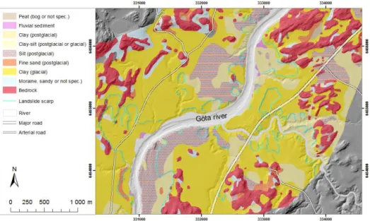
Figure 1.Landslide scarp map and Quaternary deposit map at 1:50 000 for a subregion of the Göta Älv valley.
they reach a higher spatial frequency north of Lilla Edet (AA.VV., 2012), where the majority of landslides are local-ized. The narrow northern part of the valley is predominantly covered by glacial fine clay while the central part by post-glacial silt and post-glacial/post-post-glacial clay (Fig. 1). In the south-ern part of the valley glacial clay sediments are confined to the valley sides in the proximity of the bedrock outcrops, whereas post-glacial clay sediments cover the main part of the valley floor.
3 Methodology
3.1 Description of the algorithm and of the post-processing filtering
The first computer implementation adopted in Sweden to produce landslide susceptibility maps by identifying areas above a specified cross-sectional angle used the visibility erator of ArcGIS (ESRI, Redlands, CA). The visibility op-erator is able to detect areas above a given altitude angle (our cross-sectional angle threshold). Our algorithm is in-stead based on a locally limited operator that is applied it-eratively. Rather than searching for surrounding cells above a given altitude angle, the operator checks whether the cen-tral cell rises above the given cross-sectional angle to any of the surrounding cells (the eight closest cells are exam-ined). If the cell is above neighboring cells and contains po-tentially unstable soil it is, for the calculations, reassigned a topographic height corresponding to the critical elevation. The procedure is iterated until a global solution (i.e., stable solution) is reached. This iterative scheme allows the use of several cross-sectional angle thresholds (hypothetically, one for each soil type) and (sparse) information on depth
to bedrock, something that is not as straightforward to im-plement in the classical visibility approach. The bedrock to-pography may act as a barrier, blocking line of sight, and thus reducing the area affected by a possible landslide (Tryg-gvason et al., 2015). Specifically, the steps executed in the algorithm are the following: the algorithm checks whether a cell is within soils that can be affected by landslides; if it is, the algorithm checks whether the cross-sectional an-gle calculated between the cell and its surrounding cells is steeper than the cross-sectional angle threshold; if it is, the elevation of the cell is lowered until the cross-sectional angle calculated between the cell and its surrounding cells equals the cross-sectional angle threshold. If the bedrock surface is reached, the elevation is lowered no further. The final solu-tion is reached when no further change in elevasolu-tion occurs (Tryggvason et al., 2015).
Once the algorithm results are pre-filtered the two other fil-tering criteria can be successfully applied.
3.2 Data description
We used the following map data in our analysis: DEM, soil deposits, depth to bedrock, quick-clay susceptibility index (QCSI), landslide scarps and probability of landslides. The DEM, soil deposit and depth to bedrock maps were used as the input raster data for the algorithm; the QCSI and land-slide scarp maps were used to derive QCSI-dependent cross-sectional angle thresholds; the landslide scarp and the proba-bility of landslide maps were used to assess the performance of the model.
The QCSI represents the probability of finding quick clay in a specific area (Persson et al., 2014). In the work of Pers-son et al. (2014), the QCSI was assessed by a multi-criteria evaluation. Several factors influencing quick clay formation were taken into account: stratigraphy, potential for ground-water flux, relative infiltration capacity, and geomorpholog-ical conditions for high groundwater flux. The resolution of the QCSI map is 50 m.
We used the NNH (Swedish acronym for “New National Elevation model”) data (Lysell, 2013) as DEM. The NNH data are produced from elevation measurements acquired by airborne laser scanners and are supplied at 2 m×2 m grid
res-olution.
The soil information was extracted from the soil layer database of the Swedish Geological Survey (SGU), which contains data on soil genesis and grain size. The map is at 1:50 000 scale and it is provided in vector format.
The depth to bedrock map is a product of SGU (Daniels and Thunholm, 2014) which is generated by analyzing and interpolating soil depth data from three different SGU databases: (1) soil depth (depth to bedrock) data from bore-holes and wells that reached the bedrock surface, (2) soil depth data from boreholes and wells that did not reach the bedrock surface, thus showing minimum assessed soil thin-ness, and (3) soil depth data for areas with little or no soil cover, extracted from several other databases that contain points indicating no soil or very thin soil (e.g., bedrock out-crop, ice striation). Our final depth to bedrock map was generated by interpolating to a 50 m uniform grid using the inverse weight distance method (Daniels and Thunholm, 2014). Where there is no information, the depth is assumed large; thus it will not influence the results in our modeling.
The landslide scarp map is a product of SGU and it is derived by image interpretation of the NNH data on screen (SGU, 2014). It was converted from a vector map to a raster matching the resolution of the DEM used.
The landslide probability map is a product of SGI – the Swedish Geotechnical Institute (AA.VV., 2012). The map was produced by calculating the factor of safety along sev-eral sections and through a stochastic analysis of the stability calculation’s governing variables (Berggren et al., 2011). The
landslide probability map shows the probability of landslide divided into five classes: negligible probability, low probabil-ity, some probabilprobabil-ity, pronounced probabilprobabil-ity, and obvious probability (AA.VV., 2012). As the time-dependent factors (e.g., changes in groundwater level and pore pressure) only slightly influenced the computation of the landslide proba-bility in the Göta Älv area, we argue that it is meaningful to compare the results of our algorithm to the SGI landslide probability map.
3.3 Cross-sectional angle thresholds
Retrogression distance of landslides in sensitive clays de-pends upon topography and soil properties: the cross-sectional angle is related to the geotechnical properties of the clays, specifically clay sensitivity (Mitchell and Markell, 1974; AA.VV., 2012). Since collecting large quantities of de-tailed geotechnical data is prohibitively expensive, we derive relationships between observed cross-sectional angles and geotechnical parameters of the observed slope. It has been shown that the QCSI values calculated in southwestern Swe-den are correlated with the sensitivity of the clay (Persson at al., 2014); we therefore used the QCSI as a proxy for the clay sensitivity. The cross-sectional angles were computed from the landslide scarp map for a subset of identified landslide scarps. Each cross-sectional angle was compared to the max-imum QCSI value for soil within the specific scarp area by plotting angle against maximum QCSI and taking the maxi-mum angle value within 13 discrete QCSI bins.
3.4 Model evaluation methodology
performance, we used two maps to validate the models: the landslide scarp map and the probability of landslides map.
The degree of agreement between the model results and the observed landslide scarps was evaluated using threshold-based sensitivity curves and prediction rate curves. Threshold-based sensitivity curves show the model’s ability to correctly classify landslides if each individual landslide is considered as one sample. We consider contiguous (poten-tial landslide) areas (scarps) on our hazard map. If a slide has been documented in this area and if over a given pro-portion (e.g., 50 %) of the cells on our map within this area are positive, the analysis is classed as correct. The threshold-based sensitivity curves show the sensitivity (i.e., percentage of correctly classified landslide scarps) versus the sensitiv-ity threshold (i.e., percentage of cells correctly classified in each single scarp). The higher the sensitivity at each sensi-tivity threshold, the higher the model performance. Predic-tion rate curves show the sensitivity versus the percentage of area classified as prone to landslides. Because the analysis is performed on raster data, the sensitivity of the prediction rate curve is computed as the ratio between the number of cells correctly classified and the total number of cells with observed landslides. Each single cell is therefore considered as one sample regardless of which landslide it belongs to. The aim of the prediction rate curves, as introduced by Chung and Fabbri (2003), is to assess the performance of the entire sus-ceptibility map. The assumption behind the prediction rate curves is that the higher the number of correctly classified landslides and the lower the area classified as susceptible to landslides, the better the performance. The susceptibility is often represented by a continuous range (e.g., [0,1]). The
prediction rate curves are computed by first sorting the sus-ceptibility level in descending order and then dividing by the total number of pixels of the study area. The obtained val-ues range from 0 to 1 and represent the portion of the study area classified as susceptible. Those values are finally put in bins with intervals of equal size and the percentage of land-slides is computed in each bin. Since our algorithm has a dichotomous output (i.e., not prone, prone to landslides), it is not possible to calculate the prediction rate curve for each single map; therefore we used the concept of the prediction rate curve to evaluate the performance of a set of maps (e.g., filtered maps). We computed the prediction rate curves by plotting the sensitivity data and total area classified as un-stable data from several maps in one graph. This means that one single point of the prediction rate curve represents the performance of one map.
The second type of validation was executed by comparing the model results with the probability of landslide map. The original five classes of the probability of landslide map were condensed into two classes: stable (negligible probability and low probability classes) and unstable (some probability, pro-nounced probability, and obvious probability). The Gilbert skill score (Gilbert, 1884; Schaefer, 1990) and the Heidke skill score (Heidke, 1926) were computed for each map. The
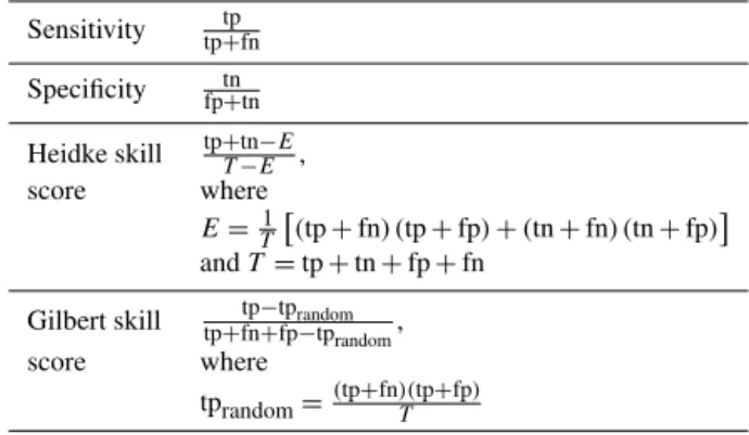
Table 1.Performance statistics. tp: true positives, tn: true negatives,
fp: false positives, fn: false negatives.Tequals total number of fore-casts, andEequals the expected number of correctly classified sam-ples due to random chance.
Sensitivity tptp+fn
Specificity fptn+tn
Heidke skill tp+tn−E T−E ,
score where
E=T1(tp+fn) (tp+fp)+(tn+fn) (tn+fp) andT=tp+tn+fp+fn
Gilbert skill tp−tprandom tp+fn+fp−tprandom,
score where
tprandom=(tp+fn)(Ttp+fp)
Gilbert skill score measures correctly classified positive sam-ples after removing true positives due to random chance (im-plying that a compensation is made for the number of used samples and the number of not correctly classified samples, see Table 1). The Heidke skill score measures correctly pre-dicted samples (both positive and negative) after removing samples which are correctly classified due to random chance (see Table 1 for the details).
4 Analysis and results
4.1 Relationship between cross-sectional angle and QCSI
In order to perform the analysis the QCSI map was interpo-lated from a 50 m×50 m pixel resolution to a 2 m×2 m pixel
resolution and the landslide scarp map was converted from vector to raster form. Cross-sectional angle values (dH/dL)
0.15 0.2 0.25 0.3 0.35 0.4 0.45 0.5 0.55 0.6 0
5 10 15 20
QCSI
Cross−sectional angle 1:n
dH/dL ratio
Cross−sectional angle upper limit
Figure 2.Relationship between the QCSI and the cross-sectional
angle computed from a subsample of the landslide scarp data.
identify an upper limit of the cross-sectional angle for a given QCSI. A similar relationship was found by comparing the cross-sectional angle values with the sensitivity of the clays (AA.VV., 2012), supporting that our approach is reasonable.
4.2 Input data and filter parameters
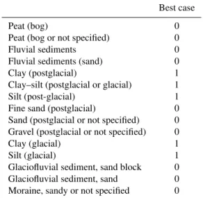
The DEM was used without further processing, whereas the depth to bedrock map was resampled to 2 m pixel size. We converted the soil map to binary form according to an SGU’s assessed likelihood that the soil type at each position contains sensitive clay (see Table 2). Soils considered potentially un-stable include clay and silt deposits of glacial or post-glacial origin. We refer to this as re-classed to produce a “best-case soil class” map, as other areas are presumed not to include any quick clay. The results were interpolated onto a 2 m×2 m
grid. SGU’s soil map was also used to produce a map con-taining combined QCSI and cross-sectional angle informa-tion for each positive cell on the best-case soil class map. This (QCSI-dependent) map was produced by using 13 sub-classes (Table 3) according to the relationship between the cross-sectional angle and the QCSI shown in Fig. 2. For ex-ample, Class 1 was assigned to pixels with QCSI lower than 0.195, Class 2 to cells with QCSI between 0.195 and 0.2, and so on.
In order to identify the optimal filter parameters we se-lected a test area and executed multiple trial runs of the pre-filter varying the neck size threshold and the parameters de-scribing the minimal area necessary for a landslide to oc-cur and the elevation difference criteria. The tests were car-ried out using the best-case scenario soil class map, with the cross-sectional angle thresholds set to 1:10 (Berggren
et al., 1991). Because the neck size is a parameter of the pre-filter aimed at separating different landslide areas, adjust-ments in the neck size were never tested alone but in combi-nation with one of the other two filters.
Table 2.Soil deposits considered unstable (1) in the best-case
sce-nario.
Best case
Peat (bog) 0
Peat (bog or not specified) 0
Fluvial sediments 0
Fluvial sediments (sand) 0
Clay (postglacial) 1
Clay–silt (postglacial or glacial) 1
Silt (post-glacial) 1
Fine sand (postglacial) 0
Sand (postglacial or not specified) 0 Gravel (postglacial or not specified) 0
Clay (glacial) 1
Silt (glacial) 1
Glaciofluvial sediment, sand block 0 Glaciofluvial sediment, sand 0 Moraine, sandy or not specified 0
Table 3.Upper limits of the QCSI used to divide the best-case soil
class in 13 subclasses and the assigned cross-sectional angle thresh-olds.
QCSI upper limit Angle
Class 1 0.195 None
Class 2 0.2 1:1
Class 3 0.21 1:3
Class 4 0.23 1:5
Class 5 0.25 1:8
Class 6 0.3 1:10
Class 7 0.32 1:13
Class 8 0.35 1:15
Class 9 0.4 1:17
Class 10 0.45 1:19
Class 11 0.5 1:20
Class 12 0.55 1:21
Class 13 1 1:22
z = 1 m z = 3 m z = 5 m z = 10 m 0.25
0.3 0.35
HSS
ma = 3 p ma = 6 p ma = 12 p ma = 24 p 0.25
0.3 0.35
HSS
Neck size 1 pixel Neck size 3 pixels Neck size 5 pixels Two times neck size 5 pixels
A
B
Figure 3.Heidke skill scores obtained by varying the elevation
dif-ference criterion(a), and the minimum area criterion(b). Results
are shown for four pre-filtering options (i.e., neck size). The eleva-tion difference criterion is given in meters (m), whereas the mini-mum area criterion in number of pixels (p).
the analysis applying the pre-filter with the neck size equal to 5 pixels and setting the elevation difference filter parame-ter equal to 5 m. Small areas were filparame-tered out by setting the minimal area threshold equal to 6 pixels (i.e., 24 m2). Fig-ure 5 shows the effect of the filtering procedFig-ure using the optimized parameters in a subarea of the study area.
4.3 Effects of depth to bedrock and filter
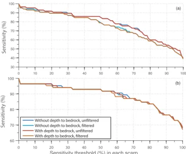
In order to study the effect of the inclusion of depth to bedrock information with and without the filtering described in the previous section, test runs each with a fixed cross-sectional angle threshold were used to analyze the best-case scenario class map. We calculated threshold-based sensitiv-ity curves for each cross-sectional angle threshold in Table 3, but we show only the results for the ratio dH/dL equal to
1:8 and 1:22 (Fig. 6). The curve calculated for the ratio
1:8 shows that the performance of the model deteriorated
when the filter was applied (Fig. 6a), since the curve of the filtered maps lies below the curve of the unfiltered maps. This was especially evident for thresholds between 40 and 80 %. This result is expected as the curves only show the correctly classified landslides and provide no information re-garding whether the classification of the stable areas has been improved or not. However, there is no difference between fil-tered and unfilfil-tered maps if the cross-sectional angle is 1:22
as shown in Fig. 6b. When taking the total area assessed to be prone to landslides into consideration, as shown in the pre-diction rate curves of Fig. 7, the performance is apparently better when the filtering is used. For cross-sectional angle thresholds between 1:8 and 1:13, the filtered maps
outper-form the maps that have not been filtered. The values of sen-sitivity are approximately the same, whereas the total area classified as prone to landslides is significantly lower for the
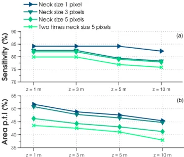
z = 1 m z = 3 m z = 5 m z = 10 m
70 75 80 85 90
Sensitivity (%)
z = 1 m z = 3 m z = 5 m z = 10 m
35 40 45 50 55
Area p.t.l (%)
Neck size 1 pixel Neck size 3 pixels Neck size 5 pixels
Two times neck size 5 pixels
(a)
(b)
Figure 4.The sensitivity(a)and area prone to landslides(b)
ob-tained by varying the elevation difference criterion. Results are shown for four pre-filtering options (i.e., neck size). The elevation difference criterion is given in meters (m).
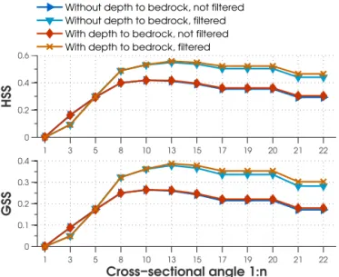
filtered maps. The use of the bedrock information does not significantly increase the performance of the filtered maps. The Gilbert skill score and the Heidke skill score (Fig. 8) show higher values (i.e., better model performance) for fil-tered than for unfilfil-tered maps. The difference in performance between the unfiltered and the filtered maps is clear for low sectional angle thresholds, whereas at high cross-sectional angle thresholds the performances are very similar. Similar conclusions can be drawn when comparing the maps obtained by with or without the depth to bedrock informa-tion. While the use of depth to bedrock information increases the value of the statistical measurements, its inclusion pro-vides a relatively small improvement to model performance when compared to the effects of using the filtering. Worth noticing is that the improvement in model performance is only evident at low values of the cross-sectional angle thresh-olds for all cases considered. In general, all four sets of maps (i.e., no bedrock/no filter, no bedrock/filter, bedrock/no filter, bedrock/filter) show similar trends in the Gilbert skill score and the Heidke skill score when the cross-sectional angle threshold is decreased: the scores reach their maximum at ratio 1:10 and 1:13 respectively and remain stable even if
the thresholds are further decreased. From this we conclude that the inclusion of the filtering procedure has a more sig-nificant effect on improving model performance compared to the addition of the depth to bedrock information.
4.4 Effects of cross-sectional angle thresholds
Figure 5.Map of area prone to landslides obtained using 1:10 as cross-sectional angle thresholds for the best-case scenario soil class. The
filtered areas were removed by using the following filtering parameters: double pre-filtering with 5-pixel neck size, elevation difference equal to 5 m, and minimal area threshold equal to 6 pixels.
0 10 20 30 40 50 60 70 80 90 100
30 40 50 60 70 80 90 100
Sensitivity (%)
0 10 20 30 40 50 60 70 80 90 100 60
70 80 90 100
Sensitivity threshold (%) in each scarp
Sensitivity (%)
Without depth to bedrock, unfiltered Without depth to bedrock, filtered With depth to bedrock, unfiltered With depth to bedrock, filtered
(a)
(b)
Figure 6.Threshold-based sensitivity curves showing the effect of
the depth to bedrock data and the filtering procedure on the areas prone to landslides with cross-sectional angle threshold equal to 1:
8(a)and equal to 1:22(b).
Table 3. Every simulation was done using two cross-sectional angle thresholds to assess whether the added information would improve results compared to when only one threshold was used. For example, for Class 7 all cells from Class 2 to 6 were assigned the cross-sectional angle threshold 1:10, and
for all cells from Class 7 to 13 the threshold 1:13 was used.
This simulation was compared to the simulation with all cells from Class 2 to 13 given the cross-sectional angle threshold 1:13. Consequently, the former simulation will identify less
0 10 20 30 40 50 60 70
0 10 20 30 40 50 60 70 80 90 100
Area p.t.l. (%)
Sensitivity (%)
Without depth to bedrock, not filtered Without depth to bedrock, filtered With depth to bedrock, not filtered With depth to bedrock, filtered 1:5
1:5 1:8
1:10
1:8 1:10 1:13
1:13
Figure 7.Prediction rate curves showing the effect of the depth
to bedrock data and the filtering procedure on the areas prone to landslides. The cross-sectional angle threshold varies from 1:1 to
1:22. The values of the cross-sectional angle thresholds are shown
for some points along the prediction rate curves.
area as prone to landslides as a higher cross-sectional angle is tolerated for part of the area than in the latter. This is seen in Fig. 9, where the curve denoted QCSI 1:13 is consequently
below the best-case 1:13 curve as fewer slides are identified.
con-1 3 5 8 10 13 15 17 19 20 21 22 0
0.2 0.4 0.6
HSS
1 3 5 8 10 13 15 17 19 20 21 22
0 0.1 0.2 0.3 0.4
Cross−sectional angle 1:n
GSS
Without depth to bedrock, not filtered Without depth to bedrock, filtered With depth to bedrock, not filtered With depth to bedrock, filtered
Figure 8. Heidke skill score and Gilbert skill score of the areas
prone to landslides obtained with or without the depth to bedrock data and with or without filtering. The effect of the depth to bedrock data and the filtering is shown for several values of the cross-sectional angle threshold (i.e., from 1:1 to 1:22).
Figure 9.Threshold-based sensitivity curves of the areas prone to
landslide obtained with cross-sectional angle thresholds either held constant for the best-case scenario soil class or dependent on the QCSI value. All the maps were obtained using the depth to bedrock data and were filtered.
sequently (except for the cross-sectional angle threshold of 1:21) never above the corresponding fixed threshold for
nei-ther of the skill scores. The QCSI information thus does not appear to improve results.
1 3 5 8 10 13 15 17 19 20 21 22
−0.2 0 0.2 0.4 0.6
HSS
Best case soil class, with depth to bedrock, filtered QCSI, with depth to bedrock, filtered
1 3 5 8 10 13 15 17 19 20 21 22
0 0.2 0.4
Cross−sectional angle 1:n
GSS
Figure 10.Heidke skill score and Gilbert skill score of the areas
prone to landslides obtained with cross-sectional angle thresholds either held constant for the best-case soil class or dependent on the QCSI value. All the maps were obtained using the depth to bedrock data and were filtered. The effect of using QCSI-dependent sectional angle thresholds is shown for several values of the cross-sectional angle threshold (i.e., from 1:1 to 1:22). Both skill scores
show that the QCSI information is not improving the results, partic-ularly in the 1:8 to 1:13 cross-sectional angle interval.
5 Discussion and conclusions
By using several methods to validate and compare the mod-eling results from running the algorithm with several settings and different filters, we have gained some insight into the performance of the algorithm and how to filter the resulting maps. In general, our results of the validation show that the algorithm has very good performance in spite of the rela-tively simple method (i.e., the method only needs two main data sources: a digital elevation model and a map of classi-fied soil deposits). The filtering procedure, wherein some ar-eas initially classified as prone to landslides are removed, is a very important step for increasing the overall performance and reducing map artifacts. However, no clear improvement is seen for high cross-sectional angles (1:1 through 1:5).
At steep cross-sectional angles the areas classified as prone to landslides are often discontinuous, and this increases the risk that they are erroneously discarded by the filtering. Also, it should be noted that as the filter parameters were optimized with a cross-sectional angle threshold of 1:10, they may not
be optimal for high cross-sectional angle thresholds. With all of this in mind, the only drawback of the filtering procedure is that it will slightly decrease the detection of areas correctly classified as prone to landslides.
for this: (1) the output of the models is very sensitive to changes in the cross-sectional angle thresholds, meaning the performance improvements gained from including the depth to bedrock data are hidden until very low angles are consid-ered; (2) the resolution (cell size) of the depth to bedrock map is 50 m meaning that it gives only a rough idea of the bedrock surface. We believe that if the analysis were performed with a depth to bedrock map at the same resolution as the DEM, the effect of the bedrock data would be more evident, which may be the case if drilling or detailed geophysical investigations were done in an area of particular interest.
Surprisingly, the use of the QCSI-dependent cross-sectional angle thresholds did not improve model perfor-mance. Since we found a relationship between the QCSI and the cross-sectional angle, we expected to obtain better per-formance by using the QCSI-dependent cross-sectional an-gle thresholds, especially when the validation was done by comparing the results of the algorithm with the landslide scarp maps. We propose two possible explanations for this: (1) the resolution of the QCSI map allows the establishment of a relationship between the QCSI values and the cross-sectional angles extracted from the landslide scarps, but it is not high enough to provide optimal results on the resolu-tion used in the performed analysis, and (2) the advantage of removing false positive detection via the QCSI-dependent cross-sectional angle thresholds may be more evident in ar-eas with low frequency of landslides.
Our results show that the optimal cross-sectional angle thresholds are between 1:8/1:10 and 1:13/1:15, with the
maximum performance reached at 1:13 in most of the cases.
This suggests that 1:13, rather than the 1:10 used generally
in Sweden, should be used as cross-sectional angle threshold in the overview mapping of areas prone to landslides.
In our test area around the Göta River there are signifi-cant quick clay deposits and many well-documented land-slides. Despite the different geological and climate areas in Sweden, we believe that conclusions based on data from this area will be generally applicable to quick clay areas through-out the country, and even in other countries where quick clay may be present. In order to proceed with the assessment of landslide susceptibility at national level, our recommenda-tions are (1) to use our algorithm as it is relatively fast and memory efficient, and allows the inclusion other information (e.g., depth to bedrock), (2) to post-filter the obtained maps to automatically remove areas falsely identified as prone to landslides and to use statistical measurements to optimize the filtering parameters, and (3) to perform the analysis us-ing the currently available depth to bedrock map as it can slightly improve the reliability of results. However, a map of the depth to bedrock with a higher resolution (<50 m pixel
size) is desirable, and (4) to further examine the use of the QCSI-dependent cross-sectional angle thresholds and evalu-ate the effect of these thresholds in areas with a lower fre-quency of landslides.
Acknowledgements. This work was financially supported by the Swedish Civil Contingencies Agency (MSB), contract 2010-2787. We would like to thank the Geological Survey of Sweden (SGU) for providing data and comments on our work. We really appreciate the help of Roland Roberts and Jean-Marc Mayotte in reviewing the language.
Edited by: F. Catani
Reviewed by: P. Quinn and one anonymous referee
References
AA.VV.: Landslide Risks in the Göta River Valley in a Chang-ing Climate, Swedish Geotechnical Institute, LinköpChang-ing, Swe-den, 164 pp., 2012.
Andersson-Sköld, Y., Torrance, J. K., Lind, B., Odén, K., Stevens, R. L., and Rankka, K.: Quick clay – a case study of chemical per-spective in southwest Sweden, Eng. Geol., 82, 107–118, 2005. Bell, R., Petschko, H., Bauer, C., Glade, T., Granica, K., Heiss, G.,
Leopold, P., Pomaroli, G., Proske, H., and Schweigl, J.: Imple-mentation of landslide susceptibility maps in Lower Austria as part of risk governance, EGU General Assembly, Vienna, Aus-tria, 27 April–2 May 2013, EGU2013-10204, 2013.
Berggren, B., Fallsvik, J., and Viberg, L.: Mapping and evaluation of landslide risk in Sweden, in: Landslides, edited by: Bell, D. H., Balkema, Rotterdam, 873–878, 1991.
Berggren, B., Alén, C., Bengtsson, P.-E., and Falemo, S.: Metodbeskrivning sannolikhet för skred: kvantitativ beräkn-ingsmodell (Description of the Method for Landslide Probabil-ity: a Quantitative Calculation), Swedish Geotechnical Institute, Linköping, Sweden, 142 ,pp., 2011.
Chung, C.-J. C. and Frabbri, A. G.: Validation of spatial prediction models for landslide hazard mapping, Nat. Hazards, 30, 451– 472, 2003.
Daniels, J. and Thunholm, B.: Rikstäckande jorddjupsmodell, Sverige (Soil Depth Model, Sweden), Geologiska Undersökning, Uppsala, Sweden, 14 pp., 2014.
Demers, D., Leroueil, S., and d’Astous, J.: Investigation of a land-slide in Maskinongé, Québec, Can. Geotech. J., 36, 1001–1014, 1999.
Erener, A., Lacasse, S., and Kaynia, A. M.: Landslide hazard map-ping by using GIS in the Lilla Edet province of Sweden, in: Proceedings of the 28th Asian Conference on Remote Sensing, Kuala Lumpur, 12–16 November 2007, 67–73, 2007.
Gilbert, G. F.: Finley’s tornado predictions, Am. Meteorol. J., 1, 166–172, 1884.
Guzzetti, F., Reichenbach, P., Ardizzone, F., Cardinali, M., and Galli, M.: Estimating the quality of landslide susceptibility mod-els, Geomorphology, 81, 166–184, 2006.
Hågeryd, A.-C., Viberg, L., and Lind, B.: Frekvens av skred i Sverige (Landslide Frequency in Sweden), Swedish Geotechni-cal Institute, Linköping, Sweden, Varia 583, 16 pp., 2007. Hågeryd, A.-C., Viberg, L., and Lind, B.: Frekvens av skred i
Heidke, P.: Berechnung des Erfolges und der Güte der Wind-stärkevorhersagen im Sturmwarnungdienst (Calculation of the success and goodness of strong wind forecasts in the storm warn-ing service), Geogr. Ann., 8, 301–349, 1926.
Høst, J., Derron, M.-H., and Sletten, K.: Digital rock-fall and snow avalanche susceptibility mapping of Norway, in: Landslide Sci-ence and Practice, edited by: Margottini, C., Canuti, P., and Sassa, K., Springer, Berlin, Heidelberg, 313–319, 2013. Karlsson, R. and Hansbo, S.: Soil Classification and Identification,
Document D8:1989, Byggforskningsrådet, Stockholm, 1989. Larsson, R., Bengtsson, P.-E., and Edstam, T.: Vägbyggande
med hänsyn till omgivningens stabilitet (Road Construction with Respect to Slope Stability), Vägverket Region Väst Dnr AL90 B 2007:27435, Swedish Geotechnical Institute slutrapport, Linköping, 32 pp., 2008.
LESSLOSS: Application of Landslides Zonation Techniques to Study Areas, Sixth Framework Programme, Priority 1.1.6.3: Global Change and Ecosystems, D-94, 275 pp., 2007.
Lindberg, F., Olvmo, M., and Bergdahl, K.: Mapping areas of po-tential slope failures in cohesive soils using a shadow-casting al-gorithm – a case study from SW Sweden, Comput. Geotech., 38, 791–799, doi:10.1016/j.compgeo.2011.05.003, 2011.
Lundqvist, J. and Wohlfarth, B.: Timing and east–west correlation of south Swedish ice marginal lines during the Late Weichselian, Quaternary Sci. Rev., 20, 1127–1148, 2001.
Lundström, K. and Andersson, M.: Hazard mapping of landslides, a comparison of three different overview mapping methods in fine-grained soils, in: Proceedings of the 4th Canadian Conference on Geohazards: from Causes to Management, Presse de l’Université Laval, Quebec, 2008.
Lysell, G.: Ny Nationell Höjdmodell, NNH, Lantmäteriets Nyhets-brev, 1, Gävle, 2 pp., 2013.
Mitchell, R. J. and Markel, A. R.: Flowsliding in sensitive soils, Can. Geotech. J., 11, 11–31, 1974.
Oh, H. J. and Pradhan, B.: Applican of a neuro-fuzzy model to landslide-susceptibility mapping for shallow landslides in a trop-ical hilly area, Comput. Geosci., 37, 1264–1276, 2011.
Osterman, J.: Studies on the properties and formation of quick clays, Clay. Clay Miner., 12, 87–108, 1963.
Påsse, T.: Havsstrandens nivå förändringar i norra Halland under Holocen tid (Seashore Level Changes in Northern Halland Dur-ing the holocene), PhD thesis, Geological Department, Chalmers Technical University, Göteborg, Sweden, 174 pp., 1983. Persson, M. A., Stevens, R. L., and Lemoine, Å.: Spatial
quick-clay predictions using multi-criteria evaluation in SW Sweden, Landslides, 11, 263–279, 2014.
Quinn, P. E.: Large Landslides in Sensitive Clay in Eastern Canada and the Associated Hazard and Risk to Linear Infrastructure, PhD thesis, Queen’s University, Kingston, Canada, 437 pp., 2009.
Rankka, K., Andersson-Sköl, Y., Hulten, C., Larsson, R., Leroux, V., and Dahlin, T.: Quick Clay in Sweden, Swedish Geotechnical Institute, Linköping, Sweden, Rep. 65, 148 pp., 2004.
Schaefer, J. T.: The critical success index as an indicator of warning skill, Weather Forecast., 5, 570–575, 1990.
Stevens, R. L.: Proximal and distal glacimarine deposits in south-western Sweden: contrasts in sedimentation, Geological Society, London, Special Publications 53, 307–316, 1990.
Svedhage, K.: Stratigraphic indications of a Pleistocene/Holocene transgression in the Göta ÁUlv river valley, SW Sweden, Boreas, 14, 87–95, 1985.
Torrance, J. K.: Towards a general model of quick clay develop-ment, Sedimentology, 30, 547–555, 1983.
Torrance, J. K.: Chemistry, sensitivity and quick-clay landslide amelioration, in: Landslides in Sensitive Clays – from Geo-sciences to Risk Management, edited by: L’Heureux, J.-S., Locat, A., Leroueil, S., Demers, D., and Locat, J., Springer, Dordrecht, 15–24, 2014.
Trigila, A., Frattini, P., Casagli, N., Catani, F., Crosta, G., Esposito, C., Iadanza, C., Lagomarsino, D., Mugnozza, G. S., Segoni, S., Spizzichino, D., Tofani, V., and Lari, S.: Landslide susceptibility mapping at national scale: the Italian case study, in: Landslide Science and Practice, edited by: Margottini, C., Canuti, P., and Sassa, K., Springer, Berlin, Heidelberg, 287–295, 2013. Tryggvason, A., Melchiorre, C., and Johansson, K.: A fast and