Application of a fast and efficient algorithm to assess landslide prone areas in sensitive clays – toward landslide susceptibility assessment, Sweden

(1)

NHESSD

2, 7773–7806, 2014

Application of a fast and efficient algorithm to assess landslide prone areas

C. Melchiorre and A. Tryggvason

Title Page

Abstract Introduction

Conclusions References

Tables Figures

◭ ◮

Back Close

Full Screen / Esc

Printer-friendly Version Interactive Discussion

Discussion

P

a

per

|

Discussion

P

a

per

|

Discussion

P

a

per

|

Discussion

P

a

per

|

Nat. Hazards Earth Syst. Sci. Discuss., 2, 7773–7806, 2014 www.nat-hazards-earth-syst-sci-discuss.net/2/7773/2014/ doi:10.5194/nhessd-2-7773-2014

This discussion paper is/has been under review for the journal Natural Hazards and Earth System Sciences (NHESS). Please refer to the corresponding final paper in NHESS if available.

Application of a fast and e

_ffi

cient

algorithm to assess landslide prone areas

in sensitive clays – toward landslide

susceptibility assessment, Sweden

C. Melchiorre and A. Tryggvason

Department of Earth Science, Uppsala University, Villavägen 16, 752 36 Uppsala, Sweden

Received: 7 November 2014 – Accepted: 19 November 2014 – Published: 19 December 2014

Correspondence to: C. Melchiorre (caterina.melchiorre@geo.uu.se)

(2)

NHESSD

2, 7773–7806, 2014

Title Page

Tables Figures

◭ ◮

Back Close

Full Screen / Esc

Discussion

P

a

per

|

Discussion

P

a

per

|

Discussion

P

a

per

|

Discussion

P

a

per

|

Abstract

This work deals with susceptibility assessment in sensitive clays at national scale. The proposed methodology is based on a procedure which uses soil data and Digital El-evation Models to detect areas prone to landslides and has been applied in Sweden for several years. Specifically, we tested an algorithm which is able to detect soil and

5

slope criteria guaranteeing a faster execution compared to other implementations and an efficient filtering procedure. The adopted computational solution allows using lo-cal information on depth to bedrock and several cross-sectional angle thresholds, and therefore opens up new possibilities to improve landslide susceptibility assessment. We tested the algorithm in the Göta River valley and evaluated the effect of filtering,

10

depth to bedrock and cross-sectional angle thresholds on model performance. The thresholds were derived by analysing the relationship between landslide scarps and the Quick Clay Susceptibility Index (QCSI). The results gave us important insights on how to implement the filtering procedure, the use of depth to bedrock and the derived cross-sectional angle thresholds in landslide susceptibility assessment.

15

1 Introduction

Landslides in sensitive clays are a recognized natural hazard in Canada, Norway, and Sweden. As they occur in very gentle terrain they are a threat to human lives as well as for transportation corridors. Since landslides in sensitive clays do not show evident signs of deformation and displacement before the actual failure, landslide hazard or

20

susceptibility maps are essential tools to minimize their impact. In Sweden sensitive clays are classified as quick clays if the sensitivity (defined as the ratio between the shear strength during undrained conditions and its remoulded shear strength) is at least 50 or higher and the fully remoulded shear strength is below 0.4 kPa (Osterman, 1963; Karlsson and Hansbo, 1989).

(3)

NHESSD

2, 7773–7806, 2014

Title Page

Tables Figures

◭ ◮

Back Close

Full Screen / Esc

Discussion

P

a

per

|

Discussion

P

a

per

|

Discussion

P

a

per

|

Discussion

P

a

per

|

In the last two decades a large amount of scientific papers dealing with landslide sus-ceptibility assessment have been published, with great focus on the use of statistically and data-driven methods above others (Guzzetti at al., 2006 and references therein). Despite the wide use of statistical methods in landslide susceptibility assessment only few works dealing with landslides in sensitive clays are found in the literature (Erener

5

et al., 2007; LESSLOSS, 2007; Quinn, 2009). An increased interest in mapping land-slide susceptibility at a national level has resulted in the Geological Survey of Sweden initiating a project on the matter. Similar e_fforts have also been made in Austria, Nor-way, and Italy (Bell at al., 2013; Høst et al., 2013; Trigila et al., 2013).

In Sweden, the methodology to derive stability maps includes a first step which aims

10

at recognizing the soil and slope conditions influencing landslide occurrence (Berggren et al., 1991; Lundström and Andersson, 2007). A typical slope where landslides in sensitive clays occur is characterized by a relatively steep part close to a river or ravine which is backed by flat terrain. The surface slope angle is therefore not representative of the slope conditions in which landslides in sensitive clays occur. Berggren et al. (1991)

15

recognized that the terrain prone to landslides in sensitive clays can be discriminated from stable terrain using the ratio dH/dL, where dH is the di_fference in height between the base and the top of the slope and dL is length of the slope (i.e. retrogression distance). Whereas the calculation of the cross-sectional angle dH/dL is simple in one dimension it is not trivial in two dimensions as stable ground can act as a physical

20

obstacle influencing the computation.

In this contribution, we test an algorithm, which is able to quickly and efficiently detect soil and slope conditions (Tryggvason et al., 2015), on real data. We choose the Göta River valley as a test site. The overall aim of our work is to evaluate the performance of the algorithm and therefore its usefulness as a main modelling tool to assess landslide

25

(4)

NHESSD

2, 7773–7806, 2014

Title Page

Tables Figures

◭ ◮

Back Close

Full Screen / Esc

Discussion

P

a

per

|

Discussion

P

a

per

|

Discussion

P

a

per

|

Discussion

P

a

per

|

described in the reference), capable to remove areas not prone to landslides. Working with real data, especially high-resolution data, there will be numerous areas that violate the dH/dL criterion due to noise and/or other real or non-real topographical effects, some of which may only be a few pixels in size. Other unwanted areas identified by the algorithm could be trenches and ditches. Such artefacts most likely do not constitute

5

any real landslide hazard and should be removed in a quick and efficient (preferably automated) procedure (Lindberg et al., 2011). In order to test the full potential of the algorithm, we used an available depth to bedrock map and derived cross-sectional angle thresholds by analysing the relationship between morphological parameters of landslide scarps and the Quick Clay Susceptibility Index (QCSI).

10

Specifically, we aim at:

1. Analysing the impact of the filtering procedure on the performance of the maps.

2. Comparing the results obtained using information on the depth to bedrock with the results obtained without it.

3. Comparing the results obtained when the QCSI-dependent cross-sectional angle

15

thresholds are used as input into the algorithm with the results obtained when only the type of soil is used.

4. Giving advices on how to use the algorithm and the available data in the national program for landslide susceptibility assessment.

2 Study area and data description

20

(5)

NHESSD

2, 7773–7806, 2014

Title Page

Tables Figures

◭ ◮

Back Close

Full Screen / Esc

Discussion

P

a

per

|

Discussion

P

a

per

|

Discussion

P

a

per

|

Discussion

P

a

per

|

In Southwest Sweden the last deglaciation started approximately 14 500 years BP and lasted for at least 5000 years producing a series of ice-margin positions (Lundqvist and Wohlfarth, 2001). During this period deposition of glacimarine sediments occurred in areas below sea level. Holocene transgression has been documented at about 10 000 BP (Svedhage, 1985) and between 9000 and 7000 BP (Påsse, 1983). The

5

clay sequences deposited during the last deglaciation are typically found above ei-ther bedrock or relatively thin diamicton and sand. The clays can be laminated and interbedded with fine-sand layers in their lowermost portions and the clay-bedrock or clay-sediment contact is abrupt (Stevens, 1990).

In the Göta River valley the deposition of clay sediments began 12 000 year BP in

10

salt water when the sea level was 125 m above present level. Glacimarine sediments present different silt content and laminae in the sediment sequences which represent several depositional environments (Stevens, 1990). Coarse material lenses are also common in the sediment sequences due to periods of ice re-advancement, marine transgression and fluvial transportation.

15

During land uplift, the clay sediments deposited in salt water underwent intense leaching by fresh water. Leaching is one the factor influencing quick clay formation (Torrance, 1983; Andersson-Sköld et al., 2005; Torrance, 2014) and it has been recog-nized as a very important factor in quick clay formation in the Göta River valley (Rankka et al., 2004). Quick clays are common in the whole valley and they reach a higher

spa-20

tial frequency North of Lilla Edet (AA.VV., 2012), where the majority of landslides are localized. The narrow Northern part of the valley is predominantly covered by glacial fine clay while the central part by post glacial silt and glacial/post glacial clay (Fig. 1). In the Southern part of the valley glacial clay sediments are confined to the valley sides in the proximity of the bedrock outcrops whereas postglacial clay sediments cover the

25

(6)

NHESSD

2, 7773–7806, 2014

Title Page

Tables Figures

◭ ◮

Back Close

Full Screen / Esc

Discussion

P

a

per

|

Discussion

P

a

per

|

Discussion

P

a

per

|

Discussion

P

a

per

|

3 Methodology

This section describes the methodology used to evaluate the potential usefulness of the algorithm in landslide susceptibility assessment. After presenting the algorithm and the data we will describe how QCSI-dependent cross-sectional angle thresholds were obtained and how model performance that is influenced by depth to bedrock data,

5

QCSI dependent cross-sectional angle thresholds, and filtering was analysed.

3.1 Description of the algorithm and of the post-processing filter

The first computational solution adopted in Sweden to detect areas above a specified dH/dL threshold was the visibility operator of ArcGIS. The visibility operator is able to detect areas which are visible from a defined point (i.e. the observation location). Our

10

algorithm is based on the visibility concept except that the visibility operator is applied locally (i.e. only on the neighbouring cells) and then iterated until a global solution (i.e. stable solution) is reached. The basic idea of the algorithm is to iteratively check if each single point or cell of a digital elevation model (DEM) is above (i.e. visible) or below (i.e. not visible) a defined cross-sectional angle threshold (i.e. line of sight). This

15

local solution allows using several cross-sectional angle thresholds (hypothetically, one for each cell) and sparse information on depth to bedrock which is not possible in the classical visibility approach. Specifically, the steps executed by the algorithm are the following: the algorithm checks if a cell is within soils that can be affected by landslides; if it is, the algorithm checks if the cross-sectional angle calculated between the cell

20

and its surrounding cells is steeper than the cross-sectional angle threshold; if it is, the elevation of the cell is lowered until the cross-sectional angle calculated between the cell and its surrounding cells equals the cross-sectional angle threshold. The elevation is lowered, at most, to the depth to bedrock if and only if data on depth to bedrock are available. To obtain a global solution this procedure is applied iteratively to each single

25

(7)

NHESSD

2, 7773–7806, 2014

Title Page

Tables Figures

◭ ◮

Back Close

Full Screen / Esc

Discussion

P

a

per

|

Discussion

P

a

per

|

Discussion

P

a

per

|

Discussion

P

a

per

|

The raw output of the algorithm, especially when a high resolution DEM is used, shows areas marked as prone to landslides which clearly should not be marked as such, either because they are too small or because they are human artefacts (e.g. ditches). A filtering procedure was therefore introduced in order to automatically remove these areas. The filter is based either on a size criterion or an elevation di_ff

er-5

ence criterion. Specifically, areas are removed if they are smaller than a defined areal threshold or the difference between the highest and the lowest point is below a de-fined elevation threshold. Erroneously detected areas that resemble two or more areas connected by a small corridor or several small corridors are difficult to remove by only using these two filters as they first need to be split into smaller areas by removing the

10

corridors interconnecting them. Therefore, these areas need to be pre-filtered. Search-ing for corridors is computationally solved by searchSearch-ing for areas classified as prone to landslides which are surrounded by stable areas. The size of corridors is defined by the pre-filter parameter called neck size. Typically a neck width of a few samples (1– 7) successfully divides these areas into smaller areas and makes them susceptible to

15

subsequent filtering. Once the algorithm results are pre-filtered the two ad hoc filtering criteria can be successfully applied.

3.2 Data description

We used the following maps in our analysis: DEM, soil deposits, depth to bedrock, QCSI, landslide scarps and probability of landslides. The DEM, soil deposit and depth

20

to bedrock maps were used as the input raster data of the algorithm; the QCSI and landslide scarp maps were used to derive QCSI-dependent cross-sectional angle thresholds; the landslide scarp and the probability of landslide maps were used to assess the performance of the model.

We used the NNH data (Lysell, 2013) as DEM. The NNH data are produced from

25

(8)

NHESSD

2, 7773–7806, 2014

Title Page

Tables Figures

◭ ◮

Back Close

Full Screen / Esc

Discussion

P

a

per

|

Discussion

P

a

per

|

Discussion

P

a

per

|

Discussion

P

a

per

|

The soil information was extracted from the soil layer database of the Swedish Geo-logical Survey (SGU), which contains data on soil genesis and granulometry. The map is at 1 : 50 000 scale.

The depth to bedrock map is a product of SGU which is generated by analysing and interpolating soil depth data from three di_fferent SGU’s databases: soil depth data

in-5

dicating the distance between the topographical surface and the bedrock; soil depth data indicating the distance between the topographical surface and a point above the bedrock and soil depth data indicating an approximately null soil depth. The first two types of data were extracted from the borehole and well databases. Data type one was extracted from boreholes and wells that reached the bedrock surface. Data type

10

two was extracted from boreholes and wells that did not reach the bedrock surface. Data type three was extracted from several other databases which contain points in-dicating no soil or very thin soil (e.g. bedrock outcrop, ice striation). The final depth to bedrock map was generated by interpolating soil depth information where the soil type is homogeneous using the inverse weight distance method, then the interpolation was

15

executed with the TOPOGRID function in order to create the final depth to bedrock surface (Daniels and Thunholm, 2014). The resolution of the map is 50 m pixel size.

The QCSI value represents the spatial probability to find quick clays in a specific area (Persson et al., 2014). In the work of Persson et al. (2014), the QCSI was assessed by a multi-criteria evaluation. Several factors influencing quick clay formation were taken

20

into account: stratigraphy, potential for ground water flux, relative infiltration capacity, and geomorphological conditions for high groundwater flux. The resolution of the QCSI map is 50 m.

The landslide scarp map is a product of SGU and it is derived by manual interpreta-tion of the NNH data.

25

(9)

im-NHESSD

2, 7773–7806, 2014

Title Page

Tables Figures

◭ ◮

Back Close

Full Screen / Esc

Discussion

P

a

per

|

Discussion

P

a

per

|

Discussion

P

a

per

|

Discussion

P

a

per

|

portant in the Göta River valley, the probability of landslide is basically the probability of failure. The landslide probability map shows the probability of landslide divided into 5 classes: negligible probability, low probability, some probability, pronounced probability, and obvious probability (AA.VV., 2012).

3.3 Cross-sectional angle thresholds

5

The retrogression distance of landslides in sensitive clays, and therefore the cross-sectional angle, is strongly related to the geotechnical parameters of the clays (Mitchell and Markell, 1973) and it was found to be correlated with the clay sensitivity (AA.VV., 2012). Since collecting geotechnical data to assess landslide susceptibility is a pro-hibitively expensive at small scale, we tested an alternative method to derive

rela-10

tionships between cross-sectional angles and geotechnical parameters. Since it was shown that the QCSI values calculated in Southwest Sweden are correlated to the sensitivity of the clay (Persson at al., 2014), we used the QCSI as proxy for the clay sensitivity. The cross-sectional angle values dH/dL were calculated from the landslide scarp map. First, cross-sectional profiles, representing geometrical conditions before

15

a landslide occurred, were extracted from a sub-sample of the landslide scarps; then the values of the ratio dH/dL were calculated. Finally, the relationship between the values of the ratio dH/dL, extracted from the cross-section profiles, and the maximum values of QCSI, extracted from the areas enclosed in the landslide scarps, was anal-ysed.

20

3.4 Model evaluation

Usually, the performance of a landslide susceptibility map is tested by calculating how good the map matches a landslide inventory map (i.e. observed data). Two statistical measurements are mainly used, namely sensitivity and specificity. The sensitivity is the ratio between the correctly classified positive samples and the total positive samples

25

(10)

NHESSD

2, 7773–7806, 2014

Title Page

Tables Figures

◭ ◮

Back Close

Full Screen / Esc

Discussion

P

a

per

|

Discussion

P

a

per

|

Discussion

P

a

per

|

Discussion

P

a

per

|

negative samples and the total negative samples (i.e. stable areas). See Table 1 for details on the calculation. While landslides represent observed positive cases the defi-nition of observed negative cases is not as trivial. In case of frequent and small mass movement events a reasonable estimation of the observed negative cases can be done by randomly extracting samples from areas where landslides have never occurred. In

5

case of infrequent and relatively big events this approach is not feasible, because of the high likelihood to extract potentially unstable areas. In order to overcome this prob-lem and to obtain reasonable estimations of model performance, we used two maps to validate the models: the landslide scarp map and the probability of landslide map. Several statistical measurements and validation methods were calculated to assess

10

model performance.

The degree of agreement between the model results and the observed landslide scarps was evaluated using threshold-based sensitivity curves and prediction rate curves. Threshold-based sensitivity curves show the model’s ability to correctly classify landslides if each individual landslide is considered as one sample. This assumption

15

means the sensitivity is dependent on whether a single scarp is considered correctly classified (e.g. when 50 % of the landslide scarp is considered correctly classified). Prediction rate curves show the sensitivity against the percentage of area classified as prone to landslides. Because the analysis is performed on raster data models the sensitivity of the prediction rate curve is calculated as the ratio between the number of

20

pixels correctly classified and the total number of pixels with observed landslides. Each single pixel is therefore considered as one sample regardless from which landslide it is extracted from. The aim of the prediction rate curves, as introduced by Chung and Fabbri (2003), is to assess the performance of the entire susceptibility map. The as-sumption behind the prediction rate curves is that the higher the number of correctly

25

(11)

NHESSD

2, 7773–7806, 2014

Title Page

Tables Figures

◭ ◮

Back Close

Full Screen / Esc

Discussion

P

a

per

|

Discussion

P

a

per

|

Discussion

P

a

per

|

Discussion

P

a

per

|

the total number of pixels in the total study area. The obtained values range from 0 to 1 and represent the portion of the study area classified as susceptible. Those values are finally put in bins with intervals of equal size and the percentage of landslides is calculated in each bin. Since our algorithm has a dichotomous output (i.e. not prone, prone to landslides), it is not possible to calculate the prediction rate curve for each

5

single map, therefore we used the concept of the prediction rate curve to evaluate the performance of a set of maps. We calculated the prediction rate curves by plotting the sensitivity data and total area classified as unstable data from several maps in one graph. This means that one single point of the prediction rate curve represents the performance of one map.

10

The second type of validation was executed by comparing the model results with the probability of landslide map. The original five classes of the probability of landslide map were condensed into two classes: stable (negligible probability and low probability classes) and unstable (some probability, pronounced probability, and obvious probabil-ity). The Gilbert skill score (Gilbert, 1884; Schaefer, 1990) and the Heidke skill score

15

(Heidke, 1926) were calculated for each map, whereas the Receiver Operating Char-acteristic (ROC) curve was calculated for a set of maps. The Gilbert skill score mea-sures correctly classified positive samples after removing true positives due to random chance. The Heidke skill score measure correctly predicted samples (both positive and negative) after removing samples which are correctly classified due to random chance.

20

Please refer to Table 1 for more details on the calculation of the scores. The ROC curve shows the false positive rate (1 – specificity) vs. the true positive rate (sensitivity). The higher the area below the ROC curve, the higher the prediction capability of the model.

4 Analysis and results

After introducing how the QCSI-dependent cross-sectional angle thresholds were

de-25

(12)

NHESSD

2, 7773–7806, 2014

Title Page

Tables Figures

◭ ◮

Back Close

Full Screen / Esc

Discussion

P

a

per

|

Discussion

P

a

per

|

Discussion

P

a

per

|

Discussion

P

a

per

|

focus on the influence of the depth to bedrock, the filter procedure, and the cross-sectional angle thresholds on the model performance.

4.1 Relationship between cross-sectional angle and QCSI

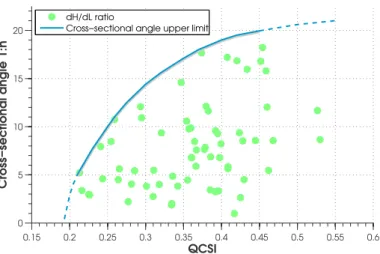
In order to perform the analysis the QCSI map was converted from a 50 m pixel resolu-tion to a 2 m pixel resoluresolu-tion and the landslide scarp map was converted from a vector

5

to a raster with a 2 m pixel size. Our original idea was to automatically extract dH and dL values for each landslide scarp and to analyse the relationship between the dH/dL ratio and the QCSI values. The dH value represents the height of the slope before the landslide event and dL value represents the maximum retrogression distance. Since it was not possible to automatically extract the dH values from all the landslides, a

sub-10

set of 71 scarps was manually selected from the database. For each of the scarps in the subset a point A on the scarp at the maximum distance (i.e. the maximum ret-rogression distance) from the scarp outlet was automatically selected. The difference in elevation, dH, was calculated between the point A and the base of the previously identified slope. For each scarp the maximum value of QCSI was extracted from the

15

area enclosed in the scarp. The relationship between the maximum QCSI value and the ratio dH/dL was then analysed (Fig. 2). Even if a clear mathematical relationship between the cross-sectional angle and the QCSI was not extractable from Fig. 2, as ex-pected, we could still identify an upper limit of the ratio dH/dL dependent on the QCSI. A similar relationship was found by comparing the cross-sectional angle values with the

20

sensitivity of the clays (AA.VV., 2012), demonstrating that our approach is reasonable.

4.2 Input data and filter parameters

The DEM was used without further processing, whereas the depth to bedrock map was resampled to 2 m pixel size. The soil map was manipulated to obtain two raster maps: a best/worst case soil class map and the QCSI-dependent soil class map. The

25

(13)

NHESSD

2, 7773–7806, 2014

Title Page

Tables Figures

◭ ◮

Back Close

Full Screen / Esc

Discussion

P

a

per

|

Discussion

P

a

per

|

Discussion

P

a

per

|

Discussion

P

a

per

|

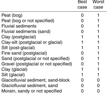
the likelihood they contain sensitive clays. The classification into the best/worst case classes was done following a classification scheme used at the SGU. Deposits with high probability to contain sensitive clays, such as clay and silt deposits of glacial or post-glacial origin, are assigned to the best case scenario soil class whereas deposits with low probability to contain sensitivity clays, such as coarse grain material, are

as-5

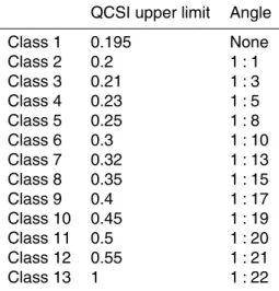
signed to the worst scenario soil class. Please refer to Table 2 for more details on the subdivision. The resulting map was converted to raster with 2 m pixel size. The QCSI-dependent soil class map was obtained by subdividing the best case scenario soil class into 13 subclasses (Table 3) according to the relationship between the dH/dL and the QCSI shown in Fig. 2.

10

In order to identify the optimal filter parameters we selected a test area from the study area and executed multiple runs of the pre-filter, which adjusted the neck size threshold, and two additional filters which adjusted the minimal area considered and the elevation di_fference criteria. The runs were done using the best case soil class, each of which were executed using no information on the depth to bedrock, while setting the

cross-15

sectional angle thresholds equal to 1 : 10. Because the neck size is a parameter of the pre-filter, adjustments in the neck size were never tested alone but in combination with one parameter of the latter two filters. The Gilbert skill score, the Heidke skill score, and the two measurements of the prediction rate curves (i.e. sensitivity and total area prone to landslides) were calculated after the filter processing. The Heidke skill score

20

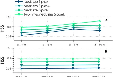
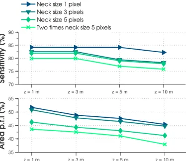
shows that the model performance continuously increases if the neck size increases, whereas it reaches the maximum when the elevation difference threshold is equal to 5 m (Fig. 3a and b). The minimal area threshold does not have any influence on the performance (Fig. 3b). The results of the Gilbert skill score are not shown since they are very similar to the Heidke skill score results. The combination of two prediction

25

(14)

NHESSD

2, 7773–7806, 2014

Title Page

Tables Figures

◭ ◮

Back Close

Full Screen / Esc

Discussion

P

a

per

|

Discussion

P

a

per

|

Discussion

P

a

per

|

Discussion

P

a

per

|

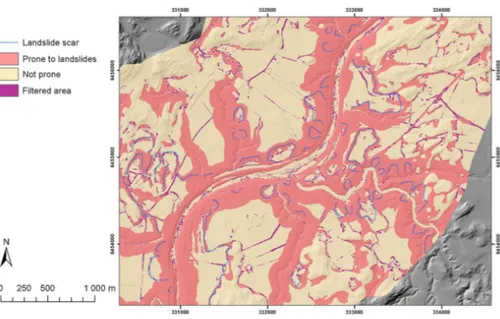
size equal to five pixels and setting the elevation difference filter parameter equal to 5 m. Small areas were filtered out by setting the minimal area threshold equal to six pixels (i.e. 24 m2). Figure 5 shows the effect of the filtering procedure, which was executed using the optimized parameters, in a subarea of the study area.

4.3 Influence of depth to bedrock, filter, and cross-sectional angle thresholds

5

on model performance

We verified how the depth to bedrock, the filter procedure, and the QCSI-dependent cross-sectional angle thresholds influence the model performance by executing multi-ple runs of the algorithm by either including or neglecting to include each in all possible combinations and then assessing model performance. These runs were executed only

10

on the areas reclassified into the best case scenario soil class. The first part of the anal-ysis aimed at studying the e_ffect of the depth to bedrock and of the filter procedure and was executed using the same cross-sectional angle threshold for the whole best case scenario class following the standard procedure used at SGU. Several cross-sectional angle thresholds were used in several algorithm runs in order to assess the e_ffect of

15

depth to bedrock and filtering on a wide range of algorithm outputs. The second part of the analysis was executed in order to assess how the QCSI-dependent cross-sectional angle thresholds influence model performance. The cross-sectional angle threshold was decreased according to the QCSI for each algorithm run. While the threshold val-ues are the same for both the first and second part of the analysis each respective

20

analysis technique used the threshold values di_fferently. The best case scenario soil class was subdivided in to 13 soil subclasses (SC) with a corresponding QCSI range and cross-sectional angle threshold (dH/dL). The array of values is presented in Ta-ble 3. For ease of explanation, we will denote each row of the array with an indexi (wherei assumes discrete values from 2 to 13). The algorithm is run for each SC(i).

25

The standard procedure examines each dH/dL(i) for the entire best case scenario soil

class, whereas during the QCSI-dependent procedure dH/dL(i) is used for SC from

(15)

NHESSD

2, 7773–7806, 2014

Title Page

Tables Figures

◭ ◮

Back Close

Full Screen / Esc

Discussion

P

a

per

|

Discussion

P

a

per

|

Discussion

P

a

per

|

Discussion

P

a

per

|

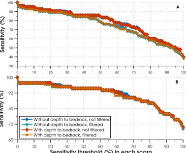
First, we show the results representing the effect of the depth to bedrock and of the filter procedure. We calculated threshold-based sensitivity curves for each cross-sectional angle threshold in Table 3, but we show only the results for the ratio dH/dL equal to 1 : 8 and 1 : 22 (Fig. 6). The curve calculated for the ratio 1 : 8 shows that the performance of the model deteriorated when the filter was applied (Fig. 6a). This

5

was especially evident for thresholds between 40 and 80 %. This result is expected as the curves show only the correctly classified landslides provides no information if the classification of the stable areas has been consequently improved or not. However, the difference between filtered and not filtered maps was annulled when the cross-sectional angle is decreased to 1 : 22 as shown in Fig. 6b. When taking the total area prone to

10

landslides into consideration, as shown in the prediction rate curves of Fig. 7, the curve for the filtered set of maps indicates that the performance is better when the filtering is used. For cross-sectional angle thresholds between 1 : 8 and 1 : 13 the filtered maps outperform the maps that have not been filtered. The values of sensitivity are approxi-mately the same, whereas the total area classified as prone to landslides is significantly

15

lower for the filtered maps. The use of the bedrock information does not significantly increase the performance of the filtered maps. The Gilbert skill score and the Heidke skill score (Fig. 8) show higher values (i.e. better model performance) for filtered out-puts than for not filtered outout-puts. The difference in performance between the not filtered and the filtered and unfiltered maps is clear for high values of the cross-sectional angle

20

thresholds, whereas at low values of the cross-sectional angle thresholds the perfor-mances are very similar. Similar conclusions can be drawn when comparing the maps obtained by using or neglecting the bedrock information. While the use of depth to bedrock information increases the value of the statistical measurements its inclusion provides a relatively small improvement to model performance when compared to the

25

(16)

NHESSD

2, 7773–7806, 2014

Title Page

Tables Figures

◭ ◮

Back Close

Full Screen / Esc

Discussion

P

a

per

|

Discussion

P

a

per

|

Discussion

P

a

per

|

Discussion

P

a

per

|

Heidke skill score when the cross-sectional angle threshold is increased: the scores reach their maximum at ratio 1 : 10 and 1 : 13 respectively and remain stable even if the thresholds are further increased. The ROC curves (not shown) show results com-parable to the Gilbert skill score and to the Heidke skill score reinforcing the conclusion that the inclusion of the filtering procedure has a more significant effect on improving

5

model performance when compared to the addition of the depth to bedrock information. In the second part of the analysis, we looked at the effect of the QCSI-dependent cross-sectional angle thresholds on model performance. The analysis was done only on the maps which used information on the depth to bedrock and underwent filter-ing. By looking at the thresholds-based sensitivity curves (Fig. 9), we notice that the

10

models obtained with the QCSI-dependent cross-sectional angle thresholds perform worse than models obtained with the standard approach. It was found that di_fferences in model performance decreased if the cross-sectional angle thresholds decreased as also shown in the earlier analyses (Fig. 6). When the total area classified as prone to landslides was also taken into account, as in the case of the prediction rate curves,

in-15

serting the cross-sectional angle thresholds neither negatively nor positively influenced the model performance. The Gilbert and Heidke skill scores (Fig. 10) show higher val-ues for the maps obtained with the standard modelling approach if the cross-sectional angle threshold is between 1 : 8 and 1 : 15. The ROC curves (not presented here) show that the maps obtained with the standard procedure and the maps obtained with the

20

QCSI-dependent modelling approach have similar performance.

5 Discussion and conclusions

By using several methods to validate the performance of the model and by running the algorithm with several settings we gained some insight into the usefulness of the algorithm and of the proposed modelling approach. In general, the results of the

vali-25

(17)

NHESSD

2, 7773–7806, 2014

Title Page

Tables Figures

◭ ◮

Back Close

Full Screen / Esc

Discussion

P

a

per

|

Discussion

P

a

per

|

Discussion

P

a

per

|

Discussion

P

a

per

|

and a map of soil deposits). The filtering procedure, wherein areas deemed not prone to landslides are removed, is a very important step for increasing overall model perfor-mance. However, the effect on model performance is not clear for high values of the cross-sectional angle (1 : 1 through 1 : 5) which we believe is due to a high frequency of discontinuous areas classified as prone to landslides. Also, it should be noted that

5

the filter parameters were optimized with a cross-sectional angle threshold of 1 : 10. With all of this in mind, the only drawback of the filtering procedure is that it will slightly decrease the detection of the positive sample.

The results show that inserting the inclusion of the depth to bedrock data does not significantly decrease the falsely detected unstable areas and that the increased model

10

performance is not as significant as the increase of model performance obtained after filtering. We believe that there are two reasons for this: (1) the output of the models is very sensitive to changes in the cross-sectional angle thresholds meaning the perfor-mance improvements gained from including the depth to bedrock data are hidden until very low angles are considered, (2) the resolution of the depth to bedrock map is 50 m

15

pixel size meaning that it gives only a rough idea of the bedrock surface. We believe that if the analysis were performed with a depth to bedrock map at the same resolution

as the DEM the e_ffect of the bedrock data would be more evident, which may be the

case if drilling or detailed geophysical investigations are done in an area of particular interest.

20

Surprisingly, the use of the QCSI-dependent cross-sectional angle thresholds did not improve model performance. Since we found a relationship between the QCSI and the

ratio dH/dL we expected to obtain better performance by using the QCSI-dependent

cross-sectional angle thresholds, especially when the validation was done by com-paring the results of the algorithm with the landslide scarp maps. We propose two

25

(18)

NHESSD

2, 7773–7806, 2014

Title Page

Tables Figures

◭ ◮

Back Close

Full Screen / Esc

Discussion

P

a

per

|

Discussion

P

a

per

|

Discussion

P

a

per

|

Discussion

P

a

per

|

QCSI-dependent cross-sectional angle thresholds may be more evident in areas with low frequency of landslides.

The results show that the optimal cross-sectional angle thresholds are between 1 : 8/1 : 10 and 1 : 13/1 : 15, with the maximum performance reached at 1 : 13 in most of the cases. This suggests that 1 : 13 should be used as cross-sectional angle

thresh-5

old in the overview mapping of area prone to landslides. In order to proceed with the assessment of landslide susceptibility at national level, we recommend:

1. Use our algorithm to perform the analysis as it guarantees a relatively fast execu-tion time, allows inserting local informaexecu-tion (e.g. depth to bedrock), and uses an efficient filtering procedure.

10

2. Use the filtering procedure to automatically remove false detected areas prone to landslides and use statistical measurements to optimize the filtering parameters.

3. Perform the analysis using the currently available depth to bedrock map as it can slightly improve the performance of the maps. However, a map of the depth to bedrock with a higher resolution (<50 m pixel size) is desirable.

15

4. Examine the use of the QCSI-dependent cross sectional angle thresholds to a greater extent. Future work could look at other ways to insert the QCSI-dependent cross-sectional angle threshold and evaluate the e_ffect of these thresh-olds in areas with a lower frequency of landslides.

Acknowledgements. This work was financially supported by the Swedish Civil Contingencies

20

(19)

NHESSD

2, 7773–7806, 2014

Title Page

Tables Figures

◭ ◮

Back Close

Full Screen / Esc

Discussion

P

a

per

|

Discussion

P

a

per

|

Discussion

P

a

per

|

Discussion

P

a

per

|

References

AA.VV.: Landslide Risks in the Göta River Valley in a Changing Climate, Swedish Geotechnical Institute, Linköping, Sweden, 164 pp., 2012.

Andersson-Sköld, Y., Torrance, J. K., Lind, B., Odén, K., Stevens, R. L., and Rankka, K.: Quick clay – a case study of chemical perspective in southwest Sweden, Eng. Geol., 82, 107–118,

5

2005.

Bell, R., Petschko, H., Bauer, C., Glade, T., Granica, K., Heiss, G., Leopold, P., Pomaroli, G., Proske, H., and Schweigl, J.: Implementation of landslide susceptibility maps in Lower Austria as part of risk governance, in: EGU General Assembly, 27 April–2 May 2013, Vienna, Austria, 2013.

10

Berggren, B., Fallsvik, J., and Viberg, L.: Mapping and evaluation of landslide risk in Sweden, in: Landslides, edited by: Bell, D. H., Balkema, Rotterdam, 873–878, 1991.

Berggren, B., Alén, C., Bengtsson, P.-E., and Falemo, S.: Metodbeskrivning sannolikhet för skred: kvantitativ beräkningsmodell (Description of the Method for Landslide Probability: a Quantitative Calculation), Swedish Geotechnical Institute, Linköping, Sweden, 142 pp.,

15

2011.

Chung, C.-J. C. and Frabbri, A. G.: Validation of spatial prediction models for landslide hazard mapping, Nat. Hazards, 30, 451–472, 2003.

Daniels, J. and Thunholm, B.: Rikstäckande jorddjupsmodell, Sverige (Soil Depth Model, Swe-den), Geologiska Undersökning, Uppsala, Sweden, 14 pp., 2014.

20

Erener, A., Lacasse, S., and Kaynia, A. M.: Landslide hazard mapping by using GIS in the Lilla Edet province of Sweden, in: Proceedings of the 28th Asian Conference on Remote Sensing, 12–16 November 2007, Kuala Lumpur, 67–73, 2007.

Gilbert, G. F.: Finley’s tornado predictions, Am. Meteorol. J., 1, 166–172, 1884.

Guzzetti, F., Reichenbach, P., Ardizzone, F., Cardinali, M., and Galli, M.: Estimating the quality

25

of landslide susceptibility models, Geomorphology, 81, 166–184, 2006.

Heidke, P.: Berechnung des Erfolges und der Güte der Windstärkevorhersagen im Sturmwar-nungdienst (Calculation of the success and goodness of strong wind forecasts in the storm warning service), Geogr. Ann., 8, 301–349, 1926.

Hågeryd, A.-C., Viberg, L., and Lind, B.: Frekvens av skred i Sverige (Landslide Frequency in

30

(20)

NHESSD

2, 7773–7806, 2014

Title Page

Tables Figures

◭ ◮

Back Close

Full Screen / Esc

Discussion

P

a

per

|

Discussion

P

a

per

|

Discussion

P

a

per

|

Discussion

P

a

per

|

Høst, J., Derron, M.-H., and Sletten, K.: Digital rock-fall and snow avalanche susceptibility map-ping of Norway, in: Landslide Science and Practice, edited by: Margottini, C., Canuti, P., and Sassa, K., Springer, Berlin, Heidelberg, 313–319, 2013.

Karlsson, R. and Hansbo, S.: Soil Classification and Identification, Document D8:1989, Byg-gforskningsrådet, Stockholm, 1989.

5

Larsson, R., Bengtsson, P.-E., and Edstam, T.: Vägbyggande med hänsyn till omgivningens stabilitet (Road Construction with Respect to Slope Stability), Vägverket Region Väst Dnr AL90 B 2007:27435, Swedish Geotechnical Institute slutrapport, Linköping, 32 pp., 2008. LESSLOSS: Application of Landslides Zonation Techniques to Study Areas, Sixth Framework

Programme, Deliverable 94, 275 pp., 2007.

10

Lindberg, F., Olvmo, M., and Bergdahl, K.: Mapping areas of potential slope failures in cohesive soils using a shadow-casting algorithm – a case study from SW Sweden, Comput. Geotech., 38, 791–799, doi:10.1016/j.compgeo.2011.05.003, 2011.

Lundqvist, J. and Wohlfarth, B.: Timing and east–west correlation of south Swedish ice marginal lines during the Late Weichselian, Quaternary Sci. Rev., 20, 1127–1148, 2001.

15

Lundström, K. and Andersson, M.: Hazard mapping of landslides, a comparison of three dif-ferent overview mapping methods in fine-grained soils, in: Proceedings of the 4th Canadian Conference on Geohazards: from Causes to Management, Presse de l’Université Laval, Quebec, 2008.

Lysell, G.: Ny Nationell Höjdmodell, NNH, Lantmäteriets Nyhetsbrev, 1, Gävle, 2 pp., 2013.

20

Mitchell, R. J. and Markel, A. R.: Flowsliding in sensitive soils, Can. Geotech. J., 11, 11–31, 1974.

Osterman, J.: Studies on the properties and formation of quick clays, Clay. Clay Miner., 12, 87–108, 1963.

Påsse, T.: Havsstrandens nivå förändringar i norra Halland under Holocen tid (Seashore Level

25

Changes in Northern Halland During the holocene), PhD thesis, Geological Department, Chalmers Technical University, Göteborg, Sweden, 174 pp., 1983.

Persson, M. A., Stevens, R. L., and Lemoine, Å.: Spatial quick-clay predictions using multi-criteria evaluation in SW Sweden, Landslides, 11, 263–279, 2014.

Quinn, P. E.: Large Landslides in Sensitive Clay in Eastern Canada and the Associated Hazard

30

(21)

NHESSD

2, 7773–7806, 2014

Title Page

Tables Figures

◭ ◮

Back Close

Full Screen / Esc

Discussion

P

a

per

|

Discussion

P

a

per

|

Discussion

P

a

per

|

Discussion

P

a

per

|

Rankka, K., Andersson-Sköl, Y., Hulten, C., Larsson, R., Leroux, V., and Dahlin, T.: Quick Clay in Sweden, Rep. 65, Swedish Geotechnical Institute, Linköping, Sweden, 148 pp., 2004. Schaefer, J. T.: The critical success index as an indicator of warning skill, Weather Forecast.,

5, 570–575, 1990.

Stevens, R. L.: Proximal and distal glacimarine deposits in southwestern Sweden: contrasts in

5

sedimentation, Special Publications 53, Geological Society, London, 307–316, 1990. Svedhage, K.: Stratigraphic indications of a Pleistocene/Holocene transgression in the Göta

ÁUlv river valley, SW Sweden, Boreas, 14, 87–95, 1985.

Torrance, J. K.: Towards a general model of quick clay development, Sedimentology, 30, 547– 555, 1983.

10

Torrance, J. K.: Chemistry, sensitivity and quick-clay landslide amelioration, in: Landslides in Sensitive Clays – from Geosciences to Risk Management, edited by: L’Heureux, J.-S., Lo-cat, A., Leroueil, S., Demers, D., and LoLo-cat, J., Springer, Dordrecht, 15–24, 2014.

Trigila, A., Frattini, P., Casagli, N., Catani, F., Crosta, G., Esposito, C., Iadanza, C., Lago-marsino, D., Mugnozza, G. S., Segoni, S., Spizzichino, D., Tofani, V., and Lari, S.:

Land-15

slide susceptibility mapping at national scale: the Italian case study, in: Landslide Science and Practice, edited by: Margottini, C., Canuti, P., Sassa, K., Springer, Berlin, Heidelberg, 287–295, 2013.

Tryggvason, A., Melchiorre, C., and Johansson, K.: A fast and efficient computer algorithm for landslide prerequisites mapping based on detailed soil and topographical information,

20

(22)

NHESSD

2, 7773–7806, 2014

Title Page

Tables Figures

◭ ◮

Back Close

Full Screen / Esc

Discussion

P

a

per

|

Discussion

P

a

per

|

Discussion

P

a

per

|

Discussion

P

a

per

|

Table 1.Table 1. Performance statistics. tp=true positives, tn=true negatives, fp=false posi-tives, fn=false negatives,T=tp+tn+fp+fn.

Sensitivity _tptp₊_fn

Specificity _fptn₊_tn

Heidke skill score tp+tn−E

T−E whereE= 1

T[(tp+fn)(tp+fp)+(tn+fn)(tn+fp)]

Gilbert skill score tp−tprandom

tp+fn+fp−tprandom where tprandom=

(23)

NHESSD

2, 7773–7806, 2014

Title Page

Tables Figures

◭ ◮

Back Close

Full Screen / Esc

Discussion

P

a

per

|

Discussion

P

a

per

|

Discussion

P

a

per

|

Discussion

P

a

per

|

Table 2.Subdivision of the soil deposits into the best case and worst case scenario soil classes.

Best Worst case case

Peat (bog) 0 1

Peat (bog or not specified) 0 1

Fluvial sediments 0 1

Fluvial sediments (sand) 0 1

Clay (postglacial) 1 1

Clay-silt (postglacial or glacial) 1 1

Silt (post-glacial) 1 1

Fine sand (postglacial) 0 1

Sand (postglacial or not specified) 0 1 Gravel (postglacial or not specified) 0 1

Clay (glacial) 1 1

Silt (glacial) 1 1

Glaciofluvial sediment, sand-block 0 0

Glaciofluvial sediment, sand 0 0

(24)

NHESSD

2, 7773–7806, 2014

Title Page

Tables Figures

◭ ◮

Back Close

Full Screen / Esc

Discussion

P

a

per

|

Discussion

P

a

per

|

Discussion

P

a

per

|

Discussion

P

a

per

|

Table 3.Upper limits of the QCSI used to divide the best case soil class in 13 subclasses and the assigned cross-sectional angle thresholds.

QCSI upper limit Angle

Class 1 0.195 None

Class 2 0.2 1 : 1

Class 3 0.21 1 : 3

Class 4 0.23 1 : 5

Class 5 0.25 1 : 8

Class 6 0.3 1 : 10

Class 7 0.32 1 : 13

Class 8 0.35 1 : 15

Class 9 0.4 1 : 17

Class 10 0.45 1 : 19

Class 11 0.5 1 : 20

Class 12 0.55 1 : 21

(25)

NHESSD

2, 7773–7806, 2014

Title Page

Tables Figures

◭ ◮

Back Close

Full Screen / Esc

Discussion

P

a

per

|

Discussion

P

a

per

|

Discussion

P

a

per

|

Discussion

P

a

per

|

(26)

NHESSD

2, 7773–7806, 2014

Title Page

Tables Figures

◭ ◮

Back Close

Full Screen / Esc

Discussion

P

a

per

|

Discussion

P

a

per

|

Discussion

P

a

per

|

Discussion

P

a

per

|

0.15 0.2 0.25 0.3 0.35 0.4 0.45 0.5 0.55 0.6

0 5 10 15 20

QCSI

Cross−sectional angle 1:n

dH/dL ratio

Cross−sectional angle upper limit

(27)

NHESSD

2, 7773–7806, 2014

Title Page

Tables Figures

◭ ◮

Back Close

Full Screen / Esc

Discussion

P

a

per

|

Discussion

P

a

per

|

Discussion

P

a

per

|

Discussion

P

a

per

|

z = 1 m z = 3 m z = 5 m z = 10 m 0.25

0.3 0.35

HSS

ma = 3 p ma = 6 p ma = 12 p ma = 24 p

0.25 0.3 0.35

HSS

Neck size 1 pixel Neck size 3 pixels Neck size 5 pixels

Two times neck size 5 pixels

A

B

(28)

NHESSD

2, 7773–7806, 2014

Title Page

Tables Figures

◭ ◮

Back Close

Full Screen / Esc

Discussion

P

a

per

|

Discussion

P

a

per

|

Discussion

P

a

per

|

Discussion

P

a

per

|

z = 1 m z = 3 m z = 5 m z = 10 m 70

75 80 85 90

Sensitivity (%)

z = 1 m z = 3 m z = 5 m z = 10 m

35 40 45 50 55

Area p.t.l (%)

Neck size 1 pixel Neck size 3 pixels Neck size 5 pixels

Two times neck size 5 pixels

(29)

NHESSD

2, 7773–7806, 2014

Title Page

Tables Figures

◭ ◮

Back Close

Full Screen / Esc

Discussion

P

a

per

|

Discussion

P

a

per

|

Discussion

P

a

per

|

Discussion

P

a

per

|

(30)

NHESSD

2, 7773–7806, 2014

Title Page

Tables Figures

◭ ◮

Back Close

Full Screen / Esc

Discussion

P

a

per

|

Discussion

P

a

per

|

Discussion

P

a

per

|

Discussion

P

a

per

|

0 10 20 30 40 50 60 70 80 90 100

30 40 50 60 70 80 90 100

Sensitivity (%)

0 10 20 30 40 50 60 70 80 90 100

60 70 80 90 100

Sensitivity threshold (%) in each scarp

Sensitivity (%)

Without depth to bedrock, not filtered Without depth to bedrock, filtered With depth to bedrock, not filtered With depth to bedrock, filtered

A

B

(31)

NHESSD

2, 7773–7806, 2014

Title Page

Tables Figures

◭ ◮

Back Close

Full Screen / Esc

Discussion

P

a

per

|

Discussion

P

a

per

|

Discussion

P

a

per

|

Discussion

P

a

per

|

0 10 20 30 40 50 60 70

0 10 20 30 40 50 60 70 80 90 100

Area p.t.l. (%)

Sensitivity (%)

1:5

1:5 1:8

1:10

1:8 1:10 1:13

1:13

(32)

NHESSD

2, 7773–7806, 2014

Title Page

Tables Figures

◭ ◮

Back Close

Full Screen / Esc

Discussion

P

a

per

|

Discussion

P

a

per

|

Discussion

P

a

per

|

Discussion

P

a

per

|

1 3 5 8 10 13 15 17 19 20 21 22

0 0.2 0.4 0.6

HSS

1 3 5 8 10 13 15 17 19 20 21 22

0 0.1 0.2 0.3 0.4

GSS

(33)

NHESSD

2, 7773–7806, 2014

Title Page

Tables Figures

◭ ◮

Back Close

Full Screen / Esc

Discussion

P

a

per

|

Discussion

P

a

per

|

Discussion

P

a

per

|

Discussion

P

a

per

|

0 20 40 60 80 100

40 50 60 70 80 90 100

Sensitivity threshold (%) in each scarp

Sensitivity (%)

Best case soil class, 1:13 Best case soil class, 1:22 QCSI, 1:13

QCSI, 1:22

(34)

NHESSD

2, 7773–7806, 2014

Title Page

Tables Figures

◭ ◮

Back Close

Full Screen / Esc

Discussion

P

a

per

|

Discussion

P

a

per

|

Discussion

P

a

per

|

Discussion

P

a

per

|

1 3 5 8 10 13 15 17 19 20 21 22

−0.2 0 0.2 0.4 0.6

HSS

Best case soil class, with depth to bedrock, filtered QCSI, with depth to bedrock, filtered

1 3 5 8 10 13 15 17 19 20 21 22

0 0.2 0.4

GSS

Application of a fast and efficient algorithm to assess landslide prone areas in sensitive clays &ndash; toward landslide susceptibility assessment, Sweden

NHESSD

Application of a fast and e

ffi

cient

algorithm to assess landslide prone areas

in sensitive clays – toward landslide

susceptibility assessment, Sweden

NHESSD

NHESSD

NHESSD

NHESSD

NHESSD

NHESSD

NHESSD

im-NHESSD

NHESSD

NHESSD

NHESSD

NHESSD

NHESSD

NHESSD

NHESSD

NHESSD

NHESSD

NHESSD

NHESSD

NHESSD

NHESSD

NHESSD

NHESSD

NHESSD

NHESSD

NHESSD

NHESSD

NHESSD

NHESSD

NHESSD

NHESSD

NHESSD

NHESSD

Application of a fast and efficient algorithm to assess landslide prone areas in sensitive clays – toward landslide susceptibility assessment, Sweden

_ffi