The Cryosphere, 7, 229–240, 2013 www.the-cryosphere.net/7/229/2013/ doi:10.5194/tc-7-229-2013
© Author(s) 2013. CC Attribution 3.0 License.
Geoscientiic
Geoscientiic
Geoscientiic
The Cryosphere
Open Access
Restoring mass conservation to shallow ice flow models over
complex terrain
A. H. Jarosch1, C. G. Schoof2, and F. S. Anslow3
1Centre for Climate and Cryosphere, Institute of Meteorology and Geophysics, University of Innsbruck, Innsbruck, Austria 2Department of Earth and Ocean Sciences, University of British Columbia, Vancouver, Canada
3Pacific Climate Impacts Consortium, University of Victoria, Victoria, Canada
Correspondence to:A. H. Jarosch ([email protected])
Received: 27 August 2012 – Published in The Cryosphere Discuss.: 21 September 2012 Revised: 21 December 2012 – Accepted: 3 January 2013 – Published: 7 February 2013
Abstract. Numerical simulation of glacier dynamics in mountainous regions using zero-order, shallow ice models is desirable for computational efficiency so as to allow broad coverage. However, these models present several difficulties when applied to complex terrain. One such problem arises where steep terrain can spuriously lead to large ice fluxes that remove more mass from a grid cell than it originally contains, leading to mass conservation being violated. This paper describes a vertically integrated, shallow ice model us-ing a second-order flux-limitus-ing spatial discretization scheme that enforces mass conservation. An exact solution to ice flow over a bedrock step is derived for a given mass balance forc-ing as a benchmark to evaluate the model performance in such a difficult setting. This benchmark should serve as a use-ful test for modellers interested in simulating glaciers over complex terrain.
1 Introduction
Numerical simulation of glaciers and ice sheets is essential for understanding the cryospheric response to a changing cli-mate and is increasingly an integral part of modern clicli-mate change projections. Although the vast majority of fresh water capable of causing sea level rise over the long-term lies in the Antarctic and Greenland ice sheets, arguably it is the moun-tain glaciers which are most susceptible to climate change in the near future. Most of them lie at moderate to high latitudes in mountainous terrain. It has been shown that these glaciers are the largest contributor to contemporary sea level rise and that they will contribute to sea level rise in the coming cen-tury (e.g. Radi´c and Hock, 2011; Marzeion et al., 2012).
This importance of alpine glaciers creates a need to un-derstand their behaviour in coming decades. One approach is to explicitly simulate glaciers at a sub-kilometer resolu-tion over large, ice-covered regions of the globe. Such an ap-proach demands models of ice dynamics capable of simulat-ing mountain glaciers in computational domains containsimulat-ing many (e.g. 107) grid nodes over century-long model periods. Higher-order ice dynamical models are capable of simulat-ing individual glaciers or large ice sheets, but presently their high computational demands restrict their use over domains required to simulate regional mountain glacier evolution. By reducing the complexity of the stresses that are simulated in a dynamical model, greater computational effort can be put into addressing large-scale problems at some cost to model accuracy. One such model is the vertically integrated, shal-low ice formulation discretized using finite differences (e.g. Mahaffy, 1976). This approach to the shallow ice problem has been used for example to simulate mountain glacier com-plexes in the Sierra Nevada, USA during the last deglaciation (Plummer and Phillips, 2003) and glacier advances on the summit of Mauna Kea, Hawaii during the last deglaciation (Anslow et al., 2010).
in modelled steady-states. This paper describes the applica-tion of a second-order flux-limiting spatial scheme to the fi-nite difference solution of a shallow ice model that ensures mass conservation. Furthermore, we describe a benchmark test case along with an exact solution upon which models can be tested for mass conservation when such situations arise. Confirming that a shallow ice model can meet the benchmark described here along with the benchmarks for the transient simulation of a growing ice sheet described by Bueler et al. (2005) is strongly recommended prior to conducting simula-tions of glaciers over rough topography.
2 Standard shallow ice models and numerical methods
In a Cartesian coordinate system with the xy-plane oriented horizontally, the continuity equation, together with Glen’s flow law (Glen, 1958), are the equations solved for the isothermal shallow ice model (Fowler and Larson, 1978; Morland and Johnson, 1980)
∂s
∂t + ∇ ·q= ˙m (1a)
q= −Ŵhn+2|∇s|n−1∇s (1b)
Ŵ=2A (ρg)
n
n+2 , (1c)
where s(x, y, t ) is ice surface elevation, h(x, y, t )=
s(x, y, t )−b(x, y)is ice thickness,b(x, y) is bed elevation andAandnare the rate factor and power law constants in Glen’s flow law, whileρ and g are ice density and accel-eration due to gravity, respectively, andm˙ is surface mass balance.∇is the 2-D gradient operator.
Importantly, Eq. (1) holds only where there is ice (h >0). Ice geometry evolution models are intrinsically free bound-ary models in which parts of the domain may be ice-free. A complete formulation of the ice flow problem must there-fore incorporate a means of evolving ice-covered and ice-free parts of the domain geometrically. In ice-free parts of the do-main,h=0 ands=b. Ice will grow ifm >˙ 0, but not other-wise. Taken together, this implies that, whenh=0,
∂s
∂t + ∇ ·q≥ ˙m. (2)
Negative ice thicknesses are never realized. In addition, at the ice margin (the free boundary between regions whereh= 0 andh >0), mass must be conserved and in addition we ex-pect the surfacesto be at least continuous. This implies
q·n=0, h=0 (3)
at this free boundary, with nnormal to the free boundary
in the xy-plane. The formulation of Eqs. (1)–(3) is known mathematically as an obstacle problem (Evans, 1998). Us-ing the inequality constraints one can re-write the problem in its so-called weak form as a variational inequality, which
allows various theoretical advances to be made, mostly in demonstrating the well-posedness of the shallow ice problem and analyzing the convergence of finite element discretiza-tions (e.g. Calvo et al., 2002; Jouvet et al., 2011; Jouvet and Bueler, 2012).
Our aim here is more practical. We address shortcom-ings in widely used numerical methods for solving shallow ice problems. A frequently used approach is to treat Eq. (1) as a parabolic (i.e. diffusion) problem, writing it in the form
∂s
∂t − ∇ ·(D∇s)= ˙m, (4)
where
D(h,|∇s|)=Ŵhn+2|∇s|n−1 (5) is a diffusion coefficient. This underlies the numerical meth-ods first developed in Mahaffy (1976) and described in more detail in Hindmarsh and Payne (1996) or Huybrechts and Payne (1996). An often used time-stepping method up-dates ice surface elevation si(x, y)=s(x, y, ti) by using a lagged diffusivityDi=D(hi,|∇si|)and solving for an un-constrained updated ice surface elevations˜i+1through
˜
si+1−si
1t − ∇ ·(D
i∇ ˜si+1)= ˙mi,
(6) where1t=ti+1−ti. This corresponds to the semi-implicit time-stepping scheme described by Hindmarsh and Payne (1996). The actual ice thickness is then updated by truncat-ing this solution anywhere the unconstrained ice surface ele-vation corresponds to negative ice thickness using a “naive” projection step such that
si+1=max(s˜i+1, b). (7)
A slightly more self-consistent approach to the inequality constraint h >0 which governs Eq. (1) would be to apply Eq. (6) only wheres˜i+1> b, and to demand instead that
˜
si+1−si
1t − ∇ ·(D
i∇ ˜si+1)≥ ˙mi+1, (8)
wheres˜i+1=0 (this essentially being the discretized version of inequality (2)), while not allowing negative s˜i+1 at all. This is mathematically equivalent of finding the updated ice thickness by minimizing the functional
J (s)˜ = Z
˜
s−si2
21t +D
i|∇ ˜s|2d, (9)
using projected successive over-relaxation (PSOR) meth-ods (Glowinski, 1984) that are similar to solving Eq. (6) with the projection step Eq. (7).
Importantly, however, the continuum formulation of Eqs. (6)–(7) as well as of Eq. (9) is misleading:Di=0 any-where the ice thicknesshi is zero, suggesting that ice flow alone should not be able to expand the ice covered area, when clearly this should be possible. In the methods de-scribed above, a spatial discretization must be applied first, and the nature of this spatial discretization is crucial.
In particular, spatial discretization schemes designed for diffusion equations of the form of Eq. (4) with bounded diffu-sivitiesDmay spuriously generate negative ice thicknesses. In fact, such methods may not be appropriate at all in set-tings where bed topography is steep. The easiest way to un-derstand this is to re-write Eq. (1) as a conservation law for ice thicknessh=s−b:
∂h ∂t − ∇ ·
h
Ŵhn+2|∇(b+h)|n−1∇(b+h)i= ˙m, (10) whereh >0, with an analogous inequality to Eq. (2) holding whereh=0. In steep terrain, the gradient term∇(b+h)may now be dominated by bed slope∇b, leading approximately to the hyperbolic problem (see also Fowler and Larson, 1978)
∂h ∂t − ∇ ·
h
Ŵhn+2|∇b|n−1∇bi= ˙m. (11) In the absence of a surface mass balance term (i.e. when
˙
m=0), this hyperbolic equation in its continuum form pre-serves positivity, i.e. given non-negative initial conditions on h, negativehwill never be generated. Spatial discretizations appropriate for hyperbolic equations will maintain this prop-erty. However, discretizations designed for parabolic prob-lems, including the symmetric centered difference schemes described in, e.g. Huybrechts and Payne (1996), may not preserve positivity forh, and can therefore spuriously gen-erate negative ice thicknesses. The projection step Eq. (7) of course will then set ice thickness back to zero where this occurs. However, in the process, this causes the numerical scheme to create mass, which can severely affect its results.
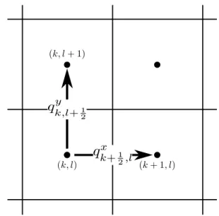
Two of the most widely used discretizations in ice sheet models are those referred to as “method 2” (abbr. M2) and “method 3” (abbr. M3) by Hindmarsh and Payne (1996) or as “type I” and “type II”1by Huybrechts and Payne (1996). All these schemes are appropriate for the primarily diffusive case of small bed slopes. Essentially, we can view these as finite volume discretizations on a regular mesh, with ice surface elevation piecewise constant on each cell. The location of cell centers are(xk, yl)on a grid with uniform spacing such that1x=xk+1−xk and1y=yl+1−yl. We label the cells by indices(k, l)and denote the normal component of flux on
1“type II” and “method 3” are actually not equivalent due to a
blunder in Huybrechts and Payne (1996).
Fig. 1.Basic grid setup and definition of fluxes.
cell boundaries such that the y-component of flux on the cell edge between cells(k, l)and(k, l+1)isqy
k,l+12 and the x-component of flux on the cell edge between cells(k, l)and (k+1, l)isqx
k+12,l(Fig. 1).
The M2 and M3 schemes both relate these fluxes to differ-ences in surface elevation through
qy,i+1 k,l+12 = −D
i k,l+12
˜
sk,li++11− ˜sk,li+1
1y (12a)
qx,i+1 k+1
2,l
= −Di k+12,l
˜
ski++11,l− ˜sk,li+1
1x , (12b)
whereDi
k,l+12 andD i
k+12,l are the diffusivities evaluated on the cell boundaries. The fully discretized version of Eq. (1a) is then
˜
sik,l+1−sk,li
1t +
qx,i+1 k+12,l−q
x,i+1
k−12,l
1x +
qy,i+1 k,l+12−q
y,i+1
k,l−12
1y = ˙m
i
k,l, (13) and the projection step Eq. (7) is applied cell-wise.
Hindmarsh and Payne’s M2 and M3 schemes only differ in how they handle the diffusivitiesDi
k,l+12 andD i
k+12,l. We define the norm of the surface gradient at the cell boundary (k+12)2in accordance with Mahaffy (1976) as
|∇si|n−1
k+1 2,l
= "
sk,li +1−sk,li −1+ski+1,l+1−sik+1,l−1
41y
2 +
ski+1,l−sk,li 1x
2#
n−1
2 (14)
2Below we give the form of diffusivities only at the cell
and can now write M2, which uses an averaged ice thickness at the cell, as
Di
k+12,l=Ŵ
hik,l+hik+1,l 2
!n+2
|∇si|n−1
k+12,l. (15) M3 uses an average over the factorhn+2that appears in the definition ofD,
Di
k+12,l=Ŵ
hik,ln+2+hik+1,ln+2 2
|∇si|n−1
k+12,l. (16) With these discretizations, the projection step scheme (cf. Eq. 7) has performed well in many ice sheet models, and in particular, has reproduced a number of known exact solu-tions outlined in Bueler et al. (2005, 2007). However, these exact benchmarks all refer to the case of a flat bed, for which we haveh=s. Our aim here is to explore a number of com-plications that arise precisely when this is not the case. That is, we wish to study complications that are typically asso-ciated with bed undulations, and which become particularly relevant for modelling mountain glaciation.
3 Mass conservation problems in projection step schemes
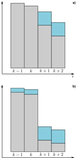
One simple yet problematic case is the one of a mountain glacier sitting in a u-shaped valley. The projection step with a M2 or M3 diffusivity can generate a spurious mass flux out of the bare rock sidewall of a u-shaped valley into a glacier in the bottom of that valley. Here, we have a cell in which hik,l=sk,li −bk,l=0 adjacent to a cell in which hik+1,l>0 and yet we also havesk,li > ski+1,l, as displayed in Fig. 2a3. That is, the ice-free cell has a higher surface elevation than the ice-covered cell. Consequently we expect thatqx
k+1 2,l
>0 and either an M2 or M3 scheme above predicts ice flowing from the ice-free into the ice-covered cell. If ice does flow out of the ice-free cell, then the time-stepping scheme (Eq. 13) will predict a negative ice thickness for the respective cell after a single time step. The projection step (Eq. 7) then sets the actual surface elevationsk,li+1 back to the bed elevation bk,l. In terms of mass conservation, we have just extracted mass from the ice-free cell(k, l)and transferred it to the ice-covered cell(k+1, l). In the projection step (Eq. 7), we have added that mass back into the cell (k, l) in a bid to avoid unphysical negative ice thickness. Formulated this way, the projection step scheme therefore creates mass.
This mass conservation issue was previously recognized by Plummer and Phillips (2003), who proposed a slightly modified scheme that prevents such a mass violation. In par-ticular, Plummer and Phillips (2003) setDi
k+12,lto either the
3Subsequently we focus on mass conservation problems along
the x-axis, but they can equally be generated in three dimensions.
M2 or M3 values suggested above except at cell boundaries that correspond to a glacier-rock wall boundary. These can be recognized as boundaries with indices(k+12, l)for which we have
(sk,li −ski+1,l)(hik,l−hik+1,l) <0 and hik,lhik+1,l=0. (17) The first of these statements says that ice thickness is greater in the cell that is at a lower elevation, while the second state-ment says that one of the cells has zero ice thickness (which must therefore be the one with the greater surface elevation). For these cell boundaries, Plummer and Phillips (2003) set Di
k+12,l=0 and they also apply an analogous scheme for Di
k,l+12 at cell boundaries parallel to the y-axis. A slightly different scheme with essentially the same properties was de-veloped independently by Haseloff (2009).
There is however another possible complication that is not captured by this adjustment of diffusivities. This can occur when a relatively thin glacier flows over a steep bedrock step, as in an icefall. Figure 2b shows the situation we have in mind. Here we can generate a significant ice flux out of the upstream grid cell(k, l)at the top of the ice fall, simply be-cause of the large surface slope between the upstream cell (k, l)and the downstream cell(k+1, l).This large flux can then lead to more ice flowing out of the grid cell (k, l) in a single time step fromti toti+1 than was present at time ti. The updated ice thickness values˜k,li+1−bk,lbecomes neg-ative after a single time step and the projection step (Eq. 7) sets itsk,li+1back to zero. Ice mass is created in the process. At timeti+2, the upstream cell is likely to acquire a non-zero ice thicknesssk,li+2again either from a positive mass balance,
˙
m >0, or through inflow from the cell(k−1, l). Such a situ-ation is possible in Plummer and Philips’ scheme. After time ti+2, we can therefore return to the same situation as timeti, with a thin ice cover in cell(k, l)and a steep surface slope into cell(k+1, l). Mass can therefore be created on alternat-ing time steps, causalternat-ing the resultalternat-ing error to grow over time. The main reason why the M2 and M3 schemes above are able to create mass in this way is that they do not limit the flux across a cell boundary as the ice thickness in the up-stream cell goes to zero. Consider a very small ice thickness hk,lin cell(k, l)whose bed elevation is greater than the sur-face elevation in the next cell downstream,bk,l> sk+1,l.
Us-inghk,l≪hk+1,landsk,l=bk,l+hk,l≈bk,l, an M2 scheme approximately gives the fluxqx
k+12,lacross the (k+
1 2, l) cell
boundary as
qx k+12,l≈Ŵ
h
k+1,l 2
n+2
sk+1,l−bk,l 1x
n−1b
k,l−sk+1,l
1x . (18)
y z
y
z a)
b)
Fig. 2.The valley glacier case in (a)and the icefall case in(b). Bedrock in grey and ice in light blue.
ice thickness in the downstream cell(k+1, l). An analogous observation applies to M3 schemes.
Below, we will illustrate this shortcoming of M2 and M3 discretizations further by showing that they fail to reproduce certain exact steady-state solutions to the shallow ice equa-tions. Before we do so, we propose an alternative scheme for computing diffusivities that restores the mass conservation.
4 A mass-conserving scheme
The difficulties of conserving mass with both M2 and M3 schemes are all rooted in the computation of the diffusivities Di
k+12,l andDk,l+12. These numerical artifacts stem from the evaluation of the ice thickness term hn+2 in the definition of diffusivity (Eq. 5). In both schemes,h on the(k+12, l) cell boundary is evaluated numerically as an average over the ice thicknesses in the adjacent cells. Consequently, the diffusivity on the cell boundary does not go to zero when the ice thickness in just one of these cells goes to zero.
When there is an advancing ice margin, it is important that the diffusivity should not go to zero at a cell boundary adjoin-ing the ice-free cell. Otherwise ice could never flow from an ice-covered cell into an ice-free cell, and the ice margin could never advance due to flow. However, we need to avoid the re-verse situation in which too much ice flows from a barely ice-covered cell into another cell with lower surface eleva-tion.
To do this, a flux-modification scheme is required. We adapt one of the flux-limiting schemes from the conservation law literature, namely a second-order Monotone Upstream-centered Schemes for Conservation Laws (MUSCL, e.g. van Leer, 1979; Gottlieb and Shu, 1998) for the ice flux dis-cretization. To do so we propose and use a new factorization of ice flux such that
q=ωhn+2 (19)
with
ω= −Ŵ|∇s|n−1∇s (20)
instead of
q= −D∇s (21)
as used in Eq. (4). This allows us to think of the shallow ice, mass continuity equation, Eq. (1), vaguely as a Burger’s equation in the form of
∂h
∂t + ∇ ·(ωh
n+2)= ˙m.
(22)
Note that Eq. (22) has the appearance of a hyperbolic conser-vation law, which is not actually the case as the gradient term
∇sthat appears in the definition ofωdepends on the
gradi-ent ofh, and the flux is at least in part diffusive. However, for steep terrain,∇smay be dominated by the bed slope∇b, and in this limiting case Eq. (22) does become hyperbolic as previously explored by Fowler and Larson (1978). Our main interest in applying a flux-limiting scheme to the shallow ice problem defined by Eq. (22) lies in the positivity-preserving property of such schemes. This prevents the spurious extrac-tion of excessive volumes of ice from grid cells in steep ter-rain that lies at the heart of the mass conservation problem identified in the previous section.
define hi
k+12−,l=h i k,l+
1
2φ (rk,l)(h i k+1,l−h
i
k,l) (23) hi
k+1 2
+
,l=h i k+1,l−
1
2φ (rk+1,l)(h i k+2,l−h
i
k+1,l) (24) hi
k−1 2
−
,l=h i k−1,l+
1
2φ (rk−1,l)(h i k,l−h
i
k−1,l) (25) hi
k−12+,l=h i k,l−
1
2φ (rk,l)(h i k+1,l−h
i
k,l) (26) with
rk,l=
hik,l−hik−1,l
hik+1,l−hik,l, (27)
the ratio of downstream to upstream ice thickness change and φ (rk,l)being the flux-limiting function. We investigate the usability of two flux limiters in our study, the minmod limiter φmm(r)and superbee limiterφsb(r)(Roe, 1986):
φmm(r)=max [0,min(1, r)] (28) φsb(r)=max [0,min(2r,1) ,min(r,2)]. (29)
Using the ice thickness estimates from Eqs. (23) and (24), we can define two flux terms at the cell boundary
Di k+1
2
+
,l=Ŵh i k+1
2
+
,l n+2
∇s
i
n−1
k+12,l (30) andDi
k+1 2
−
,l by using Eq. (23) instead of Eq. (24). To limit the flux at the cell boundary, one defines a minimum and maximum diffusivity such that
Di
k+12,l,min=min
Di
k+12−,l, D i k+12+,l
(31)
Di
k+12,l,max=max
Di
k+12−,l, D i k+12+,l
(32) and constructs a diffusivity for the(k+12, l)cell boundary as Di
k+12,l=
Di
k+12,l,min if s
i
k+1,l≤sk,li and hik+1 2
−
,l≤h i k+12+,l, Di
k+12,l,max if s
i
k+1,l≤sk,li and hik+1 2
−
,l> h i k+12+,l, Di
k+12,l,max if s
i
k+1,l> sk,li and hik+1 2
−
,l≤h i k+12+,l, Di
k+12,l,min if s
i
k+1,l> sk,li and hik+1 2
−
,l> h i k+12+,l.
(33)
The diffusivities Di k−12,l,D
i
k,l+12, and D i
k,l−12 can be con-structed in a similar manner. Note that the local surface slopes are used to identify the upstream direction, which is needed in a MUSCL scheme to assign the correct limited flux terms. We recall that our initial equation was
∂s
∂t + ∇ ·q= ˙m, (34)
which can be discretized in time, as a simpler alternative4to Eq. (6), explicitly using a forward Euler scheme
˜
si+1−si
1t − ∇ ·(D
i∇si)= ˙mi.
(35) All that is left to do is to define the gradient of the flux in its fully discretized form:
∇ ·(Di∇si)=
Di k+12,l
si k+1,l−sk,li
1x −D i k−12,l
si k,l−ski−1,l
1x
1x +
Di k,l+1
2
sk,li +1−sk,li 1y −D
i k,l−1
2
sik,l−sk,li −1 1y
1y . (36)
The value for the time step1t used is crucial in this forward scheme to provide numerically stable solutions. A stability condition can be used to automatically calculate a suitable value as
1t=cstab
min(1x2, 1y2) max(Di
k+12,l, D i k−12,l, D
i k,l+12, D
i k,l−12)
. (37)
Hindmarsh (2001) analysed time-stepping stability crite-ria and reports for explicit time-stepping schemescstab<21n
for one-dimensional andcstab<2(n1+1) for two-dimensional
configurations. In case ofn=3 this leads tocstab<0.1666˙
andcstab<0.125, respectively.
5 One-dimensional steady-states
A good way to test a shallow ice code is to compare results with exact solutions (Bueler et al., 2005, 2007). Below we construct such a steady-state solution which includes bed to-pography and a prescribed accumulation rate which is a func-tion of posifunc-tion only.
In one dimension with the assumption of steady-state, the shallow ice model (Eq. 1) can be written in the form
qx= ˙m, (38)
where the subscript “x” denotes an ordinary derivative, and q= −Ŵhn+2|sx|n−1sx. (39) To simplify matters, we assume that accumulation ratem˙ de-pends only on positionxand is such that there is a continuous ice region for the interval 0< x < xm. Herexmis the margin
position, which must be determined as part of the solution. Atx=xm,
h|x=xm=0 q|x=xm=0, (40)
4Our proposed flux-limiting scheme works well with implicit
and we have
h >0 for 0< x < xm. (41)
In addition, we assume that there is no inflow of ice at the fixed upstream boundaryx=0. In that case, ice fluxqcan be found explicitly as a function of position for any 0< x < xm:
q=
x
Z
0
˙
m(x′)dx′. (42)
To simplify our notation, we write Q(x)=Rx
0 m(x˙ ′)dx′. Givenm(x)˙ ,Q(x)is then a known function of position. The unknown margin position is then determined implicitly by the second condition in Eq. (40),
Q(xm)=0. (43)
Givenxm, ice thicknesshmust then be found as a function of
position through solving the differential equationq=Q(x), or
−Ŵhn+2|sx|n−1sx=Q(x), (44) subject to the first condition in Eq. (40),h(xm)=0.
There are no general methods for solving Eq. (44) ana-lytically. To get around this, we restrict our choice of bed topography to generate a tractable problem. Our objective is to develop a test for numerical shallow ice codes that incor-porate bed topography. Consequently, we do not wish to put b≡0. On the other hand, Eq. (44) is easiest to deal with for a flat bed, in which casesx=hx. To make use of this, we consider a bed for whichbis a step function,
b(x)=
b0 x < xs,
0 x > xs, (45)
whereb0andxs are constants, and we assume that 0< xs< xm.
In the interval 0< x < xs andxs< x < xm, this allows us
to write Eq. (44) as
−Ŵhn+2|hx|n−1hx=Q(x), (46) which we can re-write as
hn+n2hx= −
(n+
2) 2A(ρg)n
1n
|Q(x)|1n−1Q(x), (47)
where we have expandedŴaccording to Eq. (1c) for clar-ity. Integrating using the boundary conditionh(xm)=0, and
subsequently solving forh, we get h(x)=
(2n+2)(n+2)n1
2n1nA 1 nρg
xm
Z
x
|Q(x′)|1n−1Q(x′)dx′
n 2n+2
(48)
in the intervalxs< x < xm.
At the bedrock step atx=xs, we can therefore define an ice thickness just downstream of the step as
hs+= lim x→x+s
h(x)=
(2n+2) (n+2)n1
2n1nA1nρg
xm
Z
x
Q x′
1
n−1Q x′
dx′
n 2n+2
. (49)
In order to extend the solution to the interval 0< x < xs, we can then integrate Eq. (47) backwards fromx=xs:
h(x)2nn+2 =h 2n+2
n
s− + (2n+2)(n+2)1n
21nnA 1 nρg
xm
Z
x
|Q(x′)|n1−1Q(x′)dx′, (50)
wherehs−=limx→x−
s h(x). To close this solution, it remains
to determine the ice thicknesshs−at the top of the bedrock step.
In general, we expect the surface elevationsto be contin-uous. Buts=h+b, so this implies
hs−+b0=hs+ or hs−=hs+−b0. (51)
This must be substituted in Eq. (50) with hs+ given by Eq. (49).
It is, however, possible that hs− computed in this way is negative. Specifically, this occurs whenhs+computed in Eq. (49) is less thanb0. In that case, Eq. (51) cannot hold,
ashwill be negative just upstream of the bedrock step, and will therefore violate the condition given in Eq. (41). A more acceptable solution can instead be obtained in the case that hs+< b0if we puths−=0 in Eq. (50).
Allowing for this possibility, the required exact steady-state solution is given by Eqs. (50) and (48), withhs− de-termined by
hs−=max(hs+−b0,0). (52)
This solution, with a discontinuity in surface elevation, may seem an unnatural test for a shallow ice model. However, it can be shown that the solution we have given is in fact the correct limit of a solution with a continuous but steep bedrock step as the width of that bedrock step goes to zero. In numerical simulations with finite grid size, steep steps in bed topography may not be well resolved, and it is desirable to have a numerical scheme that remains robust when this is the case.
6 A specific, exact solution for a bedrock step
The solutions in Eqs. (48) and (50) are still given in terms of the general fluxQ(x)=Rx
0 m(x˙
′)dx′. Next, we give a choice Q(x) that allows us to compute h explicitly, and which is such that the corresponding accumulation rate function
˙
m=Qx(x)is sensible (in particular, which satisfies the ob-vious requirement thatQ(0)=0 and which is such thatm˙ is negative forx > xm, so that there is indeed a single ice body
in steady-state). This is given by Q(x)= m˙0
xm2n−1
xn|xm−x|n−1(xm−x) , (53)
with a corresponding accumulation rate function
˙
m(x)= nm˙0
xm2n−1
xn−1|xm−x|n−1(xm−2x) . (54) QsatisfiesQ(xm)=0, andxmcan indeed be identified with
the steady-state margin position. In additionm <˙ 0 ifx > xm,
so there is no ice outside the marginxm.
With this choice ofm˙ andQ, we have
Q x′
1
n−1Q(x′)= m˙ 1 n
0
x
2n−1 n
m
x (xm−x) , (55)
and hence the ice surface profile in Eqs. (48) and (50) can be computed as
h(x)=
(2n+2) (n+2)1nm˙ 1 n
0
21n6nA1nρgx 2n−1
n
m
(xm+2x) (xm−x)2
n 2n+2
(56) forxs < x < xm, and
h(x)=
h
2n+2 n
s− −h
2n+2 n
s+ +
(2n+2) (n+2)1nm˙ 1 n
0
21n6nA 1 nρgx
2n−1 n
m
(xm+2x) (xm−x)2
i2nn+2
(57) for 0< x < xs. Herehs+andhs−are given through the cal-culations
hs+(x) =
(2n+2) (n+2)1nm˙ 1 n
0
21n6nA 1 nρgx
2n−1 n
m
(xm+2xs) (xm−xs)2
n 2n+2
(58)
hs−(x)=max(hs+−b0,0) . (59)
7 Numerical benchmark experiments
7.1 Cliff benchmark
To demonstrate the performance of our newly introduced scheme and to showcase our exact solution as a benchmark
for numerical ice flow schemes in mountainous regions, we numerically implement Eqs. (12) and (13)5. We test three dif-ferent schemes. First, we use the diffusivity from Eq. (15) and refer to the corresponding solution as “M2” results. Sec-ondly, we compute results using the diffusivity from Eq. (30) along with the superbee flux limiter, Eq. (29). We label this solution “MUSCL superbee”. Using the minmod flux limiter, Eq. (28), gives slightly different results, which we will dis-cuss below. Thirdly, we use a simple upstream scheme based on writing the evolution Eq. (1a) in the form
∂h
∂t + ∇ ·(hu)= ˙m, (60)
whereu= −Ŵhn+1|∇s|n−1∇s. Applying a simple
upwind-ing tohin Eq. (60) leads to the following scheme (e.g. Aðal-geirsdóttir, 2003): define an upstream ice thickness through
hupi
k+1 2,l
= hi
k,l if s i k+1,l≤s
i k,l
hik+1,l if ski+1,l> sk,li , (61) and so the diffusivity becomes
Di
k+12,l=Ŵ
hik,l−hik+1,l 2
!n+1
hupi
k+12,l
sk,li +1−sk,li −1+ski+1,l+1−ski+1,l−1 41y
!2
+
ski+1,l−sk,li 1x
!2
n−1 2
. (62)
We refer to this case as “Upstream” in Fig. 3. For temporal evolution, we solve Eq. (35) with a sufficient stability condi-tion as mencondi-tioned earlier.
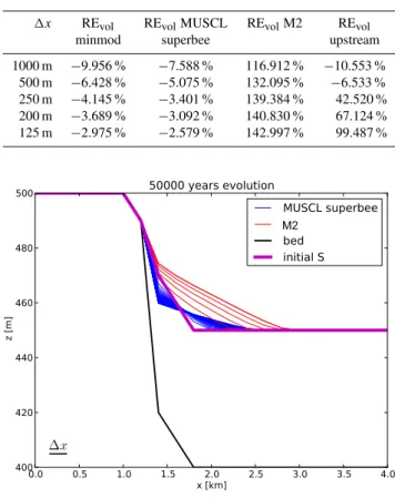
First let us define a set of parameters for the explicit solu-tion (Eqs. 56 and 57). We usexm=20 000 m,xs =7000 m, b0=500 m,m˙0=2 m yr−1,A=1×10⁻¹⁶yr−1Pa−3,n=3, ρ=910 kg m−3, andg=9.81 m s−2as well as a spatial res-olution of1x=200 m. The time-stepping stability parame-ter in Eq. (37) iscstab=0.165.
We start our numerical solutions with an initial condition of zero ice. We assume that the continuum solution should evolve toward the single steady-state solution which we have found exactly. The results of our numerical computations for the M2 scheme, the MUSCL superbee scheme, and the up-stream scheme are displayed in Fig. 3 in comparison with a result computed with Eqs. (56) and (57). We plot numeri-cal results in 1000 yr intervals for a 50 000 yr evolution of the models. The MUSCL superbee scheme (blue lines in Fig. 3) converges towards the steady-state solution (orange line in
5A Python version of the 1-D code is included in the
Fig. 3.Comparison of the “MUSCL superbee” scheme (blue lines) with a classical “M2” scheme (red lines), an upstream scheme (green lines), and a solution computed with Eqs. (56) and (57) (orange line). For all numerical schemes, solutions are plotted at 1000 yr intervals for a 50 000 yr evolution.
Fig. 3), whereas the classical M2 scheme and the upstream scheme fail to do so and create a large amount of spurious mass.
We compare volume estimates between the model outputs and the explicit solution. Integrating the steady-state solution results in a target 2-D volume of 4.539371×10⁶m2. After 50 000 yr of evolution, the “MUSCL superbee” scheme ends with a volume of 4.399017×10⁶m2, or a relative error of
−3.092 %. The classical M2 scheme leads to a volume of 10.93219×10⁶m2, or a relative error of 140.830 % and the upstream scheme to a volume of 7.586381×10⁶m2or a rel-ative error of 67.124 %. Convergence of the MUSCL scheme with both flux limiters as well as the M2 scheme and the up-stream scheme for different1xtowards the explicit solution is demonstrated in Table 1. Note that the relative error of the M2 scheme is increasing with decreasing1x. The upstream scheme displays a quite different behaviour. As long as the horizontal resolution,1x, is sufficiently larger than half the vertical bedrock step height, b0, the upstream scheme
per-forms reasonably well in the benchmark, even though not as well as either of the MUSCL schemes. As soon as1x≤b0/2
the relative volume error of the upstream scheme increases dramatically and the scheme fails the benchmark (cf. Ta-ble 1). Therefore we limit the remaining comparisons be-tween numerical schemes in the manuscript to the M2 and MUSCL schemes.
The mass conservation problem in the projection step scheme, described in Sect. 3, has been tested with our new scheme as well. We create a setup similar to the one dis-played in Fig. 2a, with as spatial resolution of1x=200 m and let it evolve for 50 000 yr withm˙ =0. The result is
dis-Table 1. Relative volume errors, REvol=(Vnumerical− Vexact)/Vexact·100, for our schemes, the M2 scheme, and the upstream scheme for different spatial resolutions. Vexact=4.546878×10⁶m2in the 2-D case described in Sect. 7 with results plotted in Fig. 3.
1x REvol REvolMUSCL REvolM2 REvol minmod superbee upstream
1000 m −9.956 % −7.588 % 116.912 % −10.553 % 500 m −6.428 % −5.075 % 132.095 % −6.533 % 250 m −4.145 % −3.401 % 139.384 % 42.520 % 200 m −3.689 % −3.092 % 140.830 % 67.124 % 125 m −2.975 % −2.579 % 142.997 % 99.487 %
M2
Fig. 4.Comparison of the “MUSCL superbee” (blue lines), with a classical “M2” scheme (red lines) for the mass conservation prob-lem described in Sect. 3. The initial surface is displayed as a ma-genta line. For both numerical schemes, solutions are plotted at 1000 yr intervals for a 50 000 yr evolution.
played in Fig. 4. We monitor the changes in ice volume, which should be zero asm˙ =0. After 50 000 yr, the solutions with the MUSCL superbee scheme (blue lines in Fig. 4) as well as the MUSCL minmod scheme (not shown) conserve mass whereas the M2 scheme has a relative volume error of
−9.5 % in comparison with the initial volume. The earlier described modification, Eq. (17), to the M2 scheme has not been applied in this comparison, which demonstrated that both of our schemes have no mass conservation difficulties in this test as well. Thus a correction step as described in Eq. (17) is not required when using our schemes.
7.2 Bueler C benchmark
50000 25000 12500 6250 3125 [m]
M2
M2
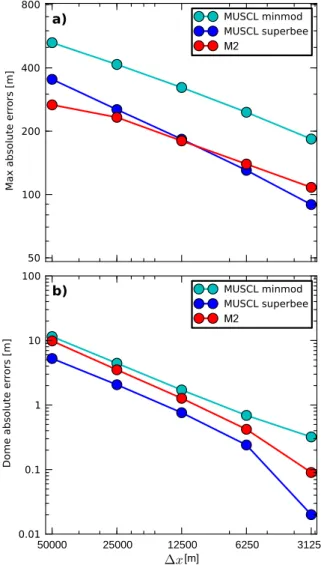
Fig. 5.Results of the Bueler C benchmark (cf. Sect. 7.2) for increas-ing spatial resolution on a log-log scale. The maximum error in the whole domain,emax, is displayed in(a), and(b)shows the central dome height erroredome.
grow an ice dome over 15 208 yr (as required by the bench-mark) after which the numerical solution is compared to the exact one. We take error in central dome ice thickness, edome=|hexact(0,0)−hnum(0,0)|, and maximum ice
thick-ness difference in the whole domain,emax=max(|hexact− hnum|), as our performance measures. Figure 5 displays the
decrease inedomeandemaxwith decreasing values of1x for
the same benchmark setup as displayed in Figs. 7 and 8 in Bueler et al. (2005).
In both cases we demonstrate that the MUSCL scheme performs better than the M2 scheme for smaller grid sizes (1x≤6250 m) if the right flux limiter is chosen, i.e. the su-perbee limiter (cf. Eq. 29). This is an anticipated result as the MUSCL scheme is second-order and thus more accurate than the M2 scheme, but it is surprising that an unfortunate choice of flux limiter, i.e. the minmod limiter (cf. Eq. 28),
makes the MUSCL scheme perform worse in comparison to the M2 scheme.
8 Conclusions
After revisiting a well-known mass conservation problem of finite difference models for glacier flow in mountainous re-gions, we have identified another complication which arises with very steep topography. In that case, several widely-used numerical schemes will extract excess mass from cells with thin ice cover, and subsequently add mass to these cells again to avoid negative ice thicknesses, thereby violating mass con-servation.
To overcome both problems, we propose using a second-order flux-limiting spatial discretization for the diffusion term in the standard shallow ice equation. In this contribution we have investigated the applicability of a MUSCL scheme with two different flux limiters, the minmod and the super-bee.
As a benchmark to evaluate the performance of the MUSCL scheme in comparison to M2 and upstream schemes in such steep topographies, we have derived an exact solu-tion to ice flow over a bedrock step for a given mass balance forcing. Using this newly derived exact solution in combina-tion with the well-established exact solucombina-tions of Bueler et al. (2005), we find the MUSCL scheme in combination with the superbee flux limiter a very suitable spatial discretization for mountain glacier flow models, which has no difficulties with the abovementioned mass conservation issues.
Our newly developed exact solution for ice flow over a bedrock step adds another exact solution-based benchmark to the existing ones (Bueler et al., 2005, 2007), against which numerical ice flow models should be evaluated. If shallow ice flow models are to be applied in mountainous regions with complex topography, we anticipate that our proposed scheme and benchmark will help significantly to improve and evalu-ate such models.
Appendix A
The failure of M2/M3 schemes in computing steady-states
With the exact solutions above in place, we can illustrate further why M2 and M3 schemes can fail. Consider the discretized steady-state shallow ice equation in one spatial dimension, discretized using a finite difference scheme as above. Using only one subscript label to indicate cells num-bered along the x-axis, we have
qk+1 2
−qk−1 2
1x = ˙mk (A1)
for an ice-covered cell, where qk+1
2
=Dk+1 2
sk+1−sk
Letqx1
2
=0, so the cell boundary to the left of the cell k=
1 is a domain boundary with no inflow, corresponding to x=0 in the continuum solutions above. Assuming that cells 1,2, . . . , kare ice covered, Eq. (A1) then shows that
qk+1 2 =
k
X
j=1
˙
mj1x, (A3)
which is analogous to the statement thatq(x)=Rx
0m(x˙ ′)dx′ in the continuum problem above.
Suppose that there is a single ice mass betweenx=0 and the marginx=xm, and that there is no ice forx > xm. Let
the discrete margin position be the cell boundary km+12,
so thathk>0 fork≤km buthk=0 fork > km, and
simi-larly qk+1
2 >0 fork≤km butqk+12 =0 for k > km.
Equa-tion (A3) of course holds only fork≤km. It can be shown
from the projection step (cf. Eq. 7) that the margin location kmin steady-state is then given by the value ofkmthat
satis-fies both of the following inequalities: km
X
j=1
˙
mj1x >0 and
km+1
X
j=1
˙
mj1x≤0, (A4)
which are equivalent to the statement thatRxm
0 m(x˙
′)dx′=0 in the continuum formulation above; it is easy to show that the margin location defined by these inequalities converges to the continuum solution ofRxm
0 m(x˙ ′)dx′.
Given a discrete margin locationkm, ice thicknesseshk fork≤km can then be computed recursively, starting with
ice thickness just upstream of the margin atk=km. For each k≤km, we have fluxqk+1
2 explicitly through Eq. (A3). To
take an example, consider a M2 discretization for diffusivity, though the argument below can also be applied in slightly modified form to a M3 discretization. Withsk=hk+bk, we then have
Ŵ
h
k+hk+1
2
n+2
hk+bk−hk+1−bk+1 1x
(n−1)
hk+bk−hk+1−bk+1
1x =qk+12 =
k
X
j=1
˙
mj1x. (A5)
This nonlinear equation must then be solved forhk, given ice thicknesshk+1at the next grid cell downstream, as well
as the bed elevationsbk andbk+1. This procedure is started
withk=km, for which we havehm+1=0.
Problems arise in this procedure if at some value ofkwe havebk> hk+1+bk+1. This occurs when surface elevation
in the(k+1)th cell is lower than bed elevation in thek-th cell. If we also demand thathk≥0, then one can show that the expression on the left-hand side of Eq. (A5) is bounded below by a quantityqminthat depends only on bed geometry
and on ice thickness downstream from the current cell, Ŵ
h
k+hk+1
2
n+2
hk+bk−hk+1−bk+1 1x
(n−1)
hk+bk−hk+1−bk+1
1x ≥Ŵ
h
k+1
2
n+2
bk−hk+1−bk+1 1x
(n−1)
bk−hk+1−bk+1 1x
=qmin(hk+1, bk, bk+1). (A6)
Hence no non-negative solution forhkcan be computed from Eq. (A5) if
qk+1
2 < qmin(hk+1, bk, bk+1).
In this situation, the assumption we have made in arriving at Eq. (A5) must break down. In particular, the assumption of a single connected ice mass in whichhk>0 fork≤kmmust
fail for the discrete solution even if it holds for the contin-uum problem, and the discrete solution will not approximate the continuous solution. Again, this occurs because the flux qk+1
2 does not go to zero even as the ice thicknesshk in the
upstream cell does.
Supplementary material related to this article is
available online at: http://www.the-cryosphere.net/7/229/ 2013/tc-7-229-2013-supplement.zip.
Acknowledgements. We would like to thank our reviewers, Ed Bueler and one anonymous reviewer, for their invaluable comments and suggestions. AHJ was supported by the Austrian Science Fund (FWF): P22443-N21. CGS was supported by a Canada Research Chair and NSERC Discovery Grant 357193. This paper is a contribution to the Western Canadian Cryospheric Network, funded by Canada Foundation for Climate and Atmospheric Sciences and a consortium of Canadian universities.
Edited by: G. H. Gudmundsson
References
Aðalgeirsdóttir, G.: Flow dynamics of Vatnajökull ice cap, Ice-land, Mitteilung 181, Versuchsantalt für Wasserbau, Hydrologie und Glaziologie der ETH Zürich-Zentrum, Ph.D. thesis, 178 pp., 2003.
Anslow, F. S., Clark, P. U., Kurz, M. D., and Hostetler, S. W.: Geochronology and paleoclimatic implications of the last deglaciation of the Mauna Kea Ice Cap, Hawaii, Earth Planet. Sc. Lett., 297, 234–248, doi:10.1016/j.epsl.2010.06.025, 2010. Bueler, E., Lingle, C. S., Kallen-Brown, J. A., Covey, D. N., and
Bueler, E., Brown, J., and Lingle, C.: Exact solutions to the thermomechanically coupled shallow-ice approximation: effective tools for verification, J. Glaciol., 53, 499–516, doi:10.3189/002214307783258396, 2007.
Calvo, N., Díaz, J., Durany, J., Schiavi, E., and Vázquez, C.: On a doubly nonlinear parabolic obstacle problem modelling ice sheet dynamics, SIAM J. Appl. Math., 63, 683–707, 2002.
Evans, L. C.: Partial Differential Equations, Graduate Studies in Mathematics, American Mathematical Society, Providence, 1998.
Fowler, A. C. and Larson, D. A.: On the flow of polythermal glaciers. I. Model and preliminary analysis, Proc. R. Soc. Lon. Ser. A, 363, 217–242, doi:10.1098/rspa.1978.0165, 1978. Glen, J. W.: The flow law of ice. A discussion of the assumptions
made in glacier theory, their experimental foundation and conse-quences, IASH, 47, 171–183, 1958.
Glowinski, R.: Numerical Methods for Nonlinear Variational Prob-lems, Springer Series in Computational Physics, Springer-Verlag, New York, 1984.
Gottlieb, S. and Shu, C.-W.: Total variation diminishing Runge-Kutta schemes, Math. Comput., 67, 73–86, doi:10.1090/S0025-5718-98-00913-2, 1998.
Haseloff, M.: Modelling the Transition between Ice Sheet and Ice Shelf with the Parallel Ice Sheet Model PISM-PIK, MSc. the-sis, Department of Physics, Humbold-Universität zu Berlin, Ger-many, 97 pp., 2009.
Hindmarsh, R. C. A.: Notes on basic glaciological computa-tional methods and algorithms, in: Continuum Mechanics and Applications in Geophysics and the Environment, edited by: Straughan, B., Greve, R., Ehrentraut, H., and Wang, Y., Springer Verlag, Berlin Heidelberg, Germany, 222–249, 2001.
Hindmarsh, R. C. A. and Payne, A. J.: Time-step limits for stable so-lutions of the ice-sheet equation, Ann. Glaciol., 23, 74–85, 1996.
Huybrechts, P. and Payne, T.: The EISMINT benchmarks for testing ice-sheet models, Ann. Glaciol., 23, 1–12, 1996.
Jouvet, G. and Bueler, E.: Steady, shallow ice sheets as obsta-cle problems: well-posedness and finite element approximation, SIAM J. Appl. Math., 72, 1292–1314, doi:10.1137/110856654, 2012.
Jouvet, G., Rappaz, J., Bueler, E., and Blatter, H.: Existence and sta-bility of steady-state solutions of the shallow-ice-sheet equation by an energy-minimization approach, J. Glaciol., 57, 345–354, 2011.
Kinderlehrer, D. and Stampacchia, G.: An Introduction to Vari-ational Inequalities and their Applications, Pure and Applied Mathematics, Academic Press, New York, 1980.
Mahaffy, M. W.: A three-dimensional numerical model of ice sheets: tests on the Barnes Ice Cap, Northwest Territories, J. Geo-phys. Res., 81, 1059–1066, 1976.
Marzeion, B., Jarosch, A. H., and Hofer, M.: Past and future sea-level change from the surface mass balance of glaciers, The Cryosphere, 6, 1295–1322, doi:10.5194/tc-6-1295-2012, 2012. Morland, L. W. and Johnson, I. R.: Steady motion of ice sheets, J.
Glaciol., 25, 229–246, 1980.
Plummer, M. A. and Phillips, F. M.: A 2-D numerical model of snow/ice energy balance and ice flow for paleoclimatic interpre-tation of glacial geomorphic features, Quaternary Sci. Rev., 22, 1389–1406, doi:10.1016/S0277-3791(03)00081-7, 2003. Radi´c, V. and Hock, R.: Regionally differentiated contribution of
mountain glaciers and ice caps to future sea-level rise, Nat. Geosci., 4, 91–94, doi:10.1038/ngeo1052, 2011.
Roe, P. L.: Characteristic-based schemes for the Eu-ler equations, Annu. Rev. Fluid Mech., 18, 337–365, doi:10.1146/annurev.fluid.18.1.337, 1986.