Geosci. Model Dev., 6, 1299–1318, 2013 www.geosci-model-dev.net/6/1299/2013/ doi:10.5194/gmd-6-1299-2013
© Author(s) 2013. CC Attribution 3.0 License.
Geoscientiic
Model Development
Open Access
Geoscientiic
Capabilities and performance of Elmer/Ice, a new-generation ice
sheet model
O. Gagliardini1,2, T. Zwinger3, F. Gillet-Chaulet1, G. Durand1, L. Favier1, B. de Fleurian1, R. Greve4, M. Malinen3, C. Martín5, P. Råback3, J. Ruokolainen3, M. Sacchettini1, M. Schäfer6, H. Seddik4, and J. Thies7
1Laboratoire de Glaciologie et Géophysique de l’Environnement, UJF-Grenoble, CNRS – UMR5183, Saint-Martin-d’Hères, France
2Institut Universitaire de France, Paris, France 3CSC-IT Center for Science Ltd., Espoo, Finland
4Institute of Low Temperature Science, Hokkaido University, Sapporo, Japan 5British Antarctic Survey, Cambridge, UK
6Arctic Centre, University of Lapland, Rovaniemi, Finland 7Uppsala University, Uppsala, Sweden
Correspondence to:O. Gagliardini ([email protected])
Received: 11 February 2013 – Published in Geosci. Model Dev. Discuss.: 4 March 2013 Revised: 8 June 2013 – Accepted: 12 July 2013 – Published: 22 August 2013
Abstract. The Fourth IPCC Assessment Report concluded that ice sheet flow models, in their current state, were un-able to provide accurate forecast for the increase of polar ice sheet discharge and the associated contribution to sea level rise. Since then, the glaciological community has un-dertaken a huge effort to develop and improve a new genera-tion of ice flow models, and as a result a significant number of new ice sheet models have emerged. Among them is the parallel finite-element model Elmer/Ice, based on the open-source multi-physics code Elmer. It was one of the first full-Stokes models used to make projections for the evolution of the whole Greenland ice sheet for the coming two cen-turies. Originally developed to solve local ice flow problems of high mechanical and physical complexity, Elmer/Ice has today reached the maturity to solve larger-scale problems, earning the status of an ice sheet model. Here, we summarise almost 10 yr of development performed by different groups. Elmer/Ice solves the full-Stokes equations, for isotropic but also anisotropic ice rheology, resolves the grounding line dynamics as a contact problem, and contains various basal friction laws. Derived fields, like the age of the ice, the strain rate or stress, can also be computed. Elmer/Ice in-cludes two recently proposed inverse methods to infer badly known parameters. Elmer is a highly parallelised code thanks to recent developments and the implementation of a block
preconditioned solver for the Stokes system. In this paper, all these components are presented in detail, as well as the nu-merical performance of the Stokes solver and developments planned for the future.
1 Introduction
As a first requisite, these models must be able to describe the ice flow heterogeneity, and particularly the major con-tribution of individual ice streams to the total ice discharge. This requires the use of an unstructured mesh in the horizon-tal plane (e.g. Gillet-Chaulet et al., 2012; Larour et al., 2012; Seddik et al., 2012) or of adaptive multi-grid methods (Corn-ford et al., 2013b). These mesh techniques are essential to produce hundred-metre-scale grid sizes in areas of interest, especially near the coast, while for the interior regions where variations in velocity gradients are small, classic grid sizes can be kept to save computing resources. Grid refinement is even more essential when considering the dynamics of the grounding line, i.e. the boundary between the grounded ice sheet and the floating ice shelf, because a grid size that is too large gives inconsistent grounding line dynamics (Du-rand et al., 2009; Pattyn et al., 2013).
The second important requisite is to have an accurate de-scription of the complex state of stress prevailing in ice streams to solve the full-Stokes system, or at least to adopt a higher-order asymptotic formulation. As shown by the ISMIP-HOM inter-comparison exercise (Pattyn et al., 2008), higher-order models are needed to describe the ice flow in ar-eas where the basal topography and slipperiness vary greatly, which are generally the most dynamic regions within ice sheets. Higher-order models are also necessary to properly describe the dynamics of the grounding line. The MISMIP inter-comparison (Pattyn et al., 2012) indicated the need to solve the full-Stokes equations near the grounding line to ob-tain fully accurate results.
The consequences of these first two requisites, i.e. high numerical resolution at places of interest and higher-order formulations, are a high computing cost and the necessity to develop parallel codes, able to run on hundreds of CPUs. Re-cent studies (Larour et al., 2012; Gillet-Chaulet et al., 2012; Seddik et al., 2012; Cornford et al., 2013b) have fulfilled these requirements and have shown that by deploying high-performance computing (HPC) techniques this challenge can be successfully taken on. In this context, Elmer/Ice takes ad-vantage of being backed by a large open-source community that also develops new numerical and HPC techniques for the code (e.g. Malinen, 2007).
The third requisite, and from the physical point of view the most challenging, is to implement physically founded bound-ary conditions. These improvements are far more complex and it will take more time to fully address them in the ice sheet flow models. The recently observed changes in coastal glacier dynamics (e.g. Moon et al., 2012) are certainly driven by changes in ice sheet and ice shelf boundary conditions, and consequently linked to changes in the ocean and atmo-sphere components of the climatic system. In the simplest cases, changes in the climatic components directly drive the changes at the boundaries of the ice mass. This is the case for surface air temperature or ocean temperature which directly drive the temperature boundary condition of the upper sur-face or the bottom ice/ocean intersur-face, respectively. In other
more complex cases, the link between changes in the ocean and/or atmosphere and changes in the ice flow is indirect. In-termediate processes (often not observable) are involved, as in the case for example of the link between surface runoff and basal sliding or ocean temperature and calving rate. Thus, a dedicated model is required to describe the processes re-sponsible for the transfer of these changes to the ice mass. Driving this dedicated transfer model might require coupling the ice sheet model with an atmosphere or an ocean model.
The last important requisite for a forecast model is to be able to simulate present-day observations with as much fi-delity as possible (Aschwanden et al., 2013). This point must be addressed clearly using data assimilation techniques and specific inverse methods to estimate the less well known pa-rameters of the model (e.g. Heimbach and Bugnion, 2009; Arthern and Gudmundsson, 2010; Morlighem et al., 2010).
only full-Stokes model able to run forecast simulations for the whole Greenland ice sheet for the coming AR5 IPPC re-port, in the framework of both SeaRISE (Seddik et al., 2012) and ice2sea (Gillet-Chaulet et al., 2012; Shannon et al., 2013; Edwards et al., 2013) programmes.
In this paper, we summarise ten years of consistent devel-opments and present the current state of the new-generation ice sheet model Elmer/Ice (Elmer library version 7.0 SVN revision 5955). We only focus on the past developments that are relevant for simulations of three-dimensional ice sheets. Specific developments regarding two-dimensional flow line or glacier applications are not presented here, but one can consult previous publications on these types of applications (the complete list of Elmer/Ice publications can be found on http://elmerice.elmerfem.org/). Section 2 presents the gov-erning equations implemented in Elmer/Ice. The associated boundary conditions are discussed in Sect. 3. Other useful equations, such as the equation to evaluate the age of the ice, are presented in Sect. 4. Section 5 is dedicated to the inverse methods implemented in Elmer/Ice. Some technical aspects related to the resolution of these equations in the framework of the FE method are discussed in Sect. 6. The efficiency of Elmer/Ice was verified by standard convergence and scal-ability tests described in Sect. 7. Finally, we provide some insights into the future planned developments in Sect. 8.
2 Governing equations
2.1 Ice flow equations
Ice is a fluid with an extremely high viscosity that flows very slowly so that inertia and acceleration terms entering the momentum equation can be neglected. Therefore, the three-dimensional velocity field and the pressure field of an ice mass flowing under gravity are obtained by solving the Stokes equations over the ice volume. The Stokes equa-tions express the conservation of linear momentum
divσ+ρg=divτ− gradp+ρg=0, (1) and the mass conservation
divu=trε˙=0. (2)
In these equations,ρ is the ice density,g=(0,0,−g) the gravity vector,u=(u, v, w)the ice velocity vector,σ=τ−
pIthe Cauchy stress tensor with p= −trσ/3 the isotropic pressure,τ the deviatoric stress tensor andIthe identity ma-trix. This system of equations of unknownsuandpis closed by adopting one of the rheological laws presented in the next section. The conditions that are applied on the boundaryŴof the volumeare discussed in Sect. 3.
2.2 Rheological laws for polar ice
Even if most ice sheet models assume an isotropic rheolog-ical law for ice, it is well known that the viscous response
of polar ice can be strongly anisotropic, and that this re-sponse depends on the crystal orientation distribution, i.e. the ice fabric (e.g. Gagliardini et al., 2009). Elmer/Ice in-cludes the classic isotropic Glen’s flow law as well as two anisotropic flow laws. As shown in various applications, the anisotropy of polar ice has a strong influence on the over-all flow (Zwinger et al., 2013) and will in turn modify the age–depth relationship (Gillet-Chaulet et al., 2006; Seddik et al., 2011). In central parts of ice sheets, ice anisotropy and the development of fabric can explain the observed hetero-geneity of the ice deformation along a drilling (Durand et al., 2007). On the coastal area, due to the large contrast of the stress regimes for the grounded part and for the ice shelf, the ice anisotropy induces an apparent hardening of the ice up to a factor 10 when ice moves from grounded to floating (Ma et al., 2010).
When ice is assumed to behave as an isotropic material, its rheology is given by a Norton–Hoff power law, known as Glen’s law in glaciology, which links the deviatoric stressτ
with the strain rateε˙:
τ=2ηε˙, (3)
where the effective viscosityηis defined as
η=1
2(EA)
−1/nε˙(1−n)/n
e . (4)
In Eq. (4),ε˙e2=tr(ε˙2)/2 is the square of the second in-variant of the strain rate andA=A(T′)is a rheological pa-rameter which depends on T′, the ice temperature relative to the pressure melting point, via an Arrhenius law. The en-hancement factorE in Eq. (4) is often used to account for anisotropy effects, by prescribing an ad hoc value depend-ing on the ice age and/or type of flow. Due to the state of stress,E is expected to be greater than 1 for grounded ice of polar ice sheets, whereas a value lower than 1 should be used for floating ice shelves (Ma et al., 2010). A compress-ible form of Glen’s law (Gagliardini and Meyssonnier, 1997), well adapted to describe the flow of firn, is also implemented in Elmer/Ice (Zwinger et al., 2007).
Both implemented anisotropic flow laws depend on the ice polycrystalline fabric, which is described by its second- and fourth-order orientation tensors a(2) and a(4), respectively,
defined as
aij(2)= hcicjiandaij kl(4) = hcicjckcli, (5)
et al., 2009). For randomcaxes distribution the non-zero en-tries ofa(2) area(2)
11 =a
(2)
22 =a
(2)
33 =1/3, for a single maxi-mum fabric with its maximaxi-mum in the third direction,a(332)>
1/3 and a(112)≈a22(2)<1/3, and for a girdle-type fabric in the plane(x1, x2),a33(2)<1/3 and a11(2)≈a(222)>1/3. In ad-dition to three eigenvalues, three Euler angles are necessary to uniquely definea(2) with respect to a general reference frame. It can be shown analytically with a linear flow that if the second- and fourth-order orientation tensors have the same eigenframe, the polycrystal behaviour will exhibit or-thotropic symmetries (Gillet-Chaulet et al., 2006). The equa-tions for the fabric evolution are presented in Sect. 2.5.
The first anisotropic flow law implemented in Elmer/Ice is the non-linear General Orthotropic Flow Law (GOLF, Gillet-Chaulet et al., 2005; Ma et al., 2010). The GOLF provides a non-collinear and non-linear relation between strain rate and stress, using the concept of structure tensors. In its initial form, the ice was assumed to behave as a linearly viscous or-thotropic material. In more recent works (Martín et al., 2009; Ma et al., 2010), the GOLF has been extended to a non-linear form by adding an invariant in the anisotropic non-linear law. The simplest choice is either to add the second invariant of the strain rateε˙e (Martín et al., 2009) or the second in-variant of the deviatoric stressτe (withτe2=tr(τ2)/2, Pettit et al., 2007; Ma et al., 2010). No theoretical or experimental results are available today to discard one of these two solu-tions, and other solutions based on anisotropic invariants of the deviatoric stress and/or the strain rate are also possible. In Elmer/Ice, both solutions are implemented. Using the sec-ond invariant of the deviatoric stress, for a given fabric and a given state of stress, the corresponding strain rate relative to the isotropic response is the same for the linear and non-linear cases. Using the strain-rate invariant in the same way as Martín et al. (2009) leads to an opposite definition of the anisotropy ratios: for a given strain rate, the corresponding stress relative to the isotropic response is the same for the linear and non-linear cases. When using the stress second in-variant, the GOLF reads
2Aτen−1τ= 3
X
r=1
h
ηrtr(Mr·ε˙)MDr +ηr+3(ε˙·Mr+Mr·ε˙)D
i
. (6)
The six dimensionless anisotropy viscositiesηr(a(2))and
ηr+3(a(2))(r=1, 2, 3) are functions of eigenvalues of the second-order orientation tensora(2), which represent a
mea-sure of the anisotropy strength. The three structure tensors
Mr are given by the dyadic products of the three
eigenvec-tors ofa(2), which then represent the material symmetry axes.
In the method proposed by Gillet-Chaulet et al. (2006), the six dimensionless viscositiesηr(a(2))are tabulated as a
func-tion of the fabric strength (i.e. thea(i2)) using a micro-macro model. Various micro-macro models, from the assumption of uniform stress within the ice polycrystal to the assumption of uniform strain rate, as well as different crystal anisotropy
can be used to tabulate the six viscositiesηr. The most
re-alistic polycrystalline response is obtained using the visco-plastic self-consistent model (VPSC, Castelnau et al., 1996, 1998), with the two crystal anisotropy parameters chosen so that the experimentally observed polycrystal anisotropy is re-produced (Gillet-Chaulet et al., 2006; Ma et al., 2010). When the ice is isotropic,ηr =0 andηr+3=1 (r=1, 2, 3), then the GOLF (6) reduces to Glen’s isotropic flow law (3) with
E=1.
The second anisotropic flow law implemented in Elmer/Ice is the Continuum-mechanical Anisotropic Flow model based on an anisotropic Flow Enhancement factor (CAFFE, Seddik et al., 2008; Placidi et al., 2010). The CAFFE model assumes collinearity between the strain rate and deviatoric stress tensors, so that the general form of Glen’s law (3) is not modified, but the enhancement factor
Eis a function of the polycrystalline deformabilityDsuch that
E(D)=
(
(1−Emin) Dt+Emin 1≥D≥0,
4D2(Emax−1)+25−4Emax
21 5/2≥D >1,
(7)
with
t= 8
21
E
max−1 1−Emin
, Emax≈10, Emin≈0.1. (8) The polycrystalline deformabilityDis a function of strain rate and fabric. WhenD=0, the minimal enhancement fac-torEminis reached, which corresponds to an uni-axial com-pression on a single maximum fabric. For an isotropic fab-ric,D=1 and the response is identical whatever the strain rate, whereas the maximal enhancementEmaxis obtained for
D=5/2, which corresponds to a single maximum fabric un-dergoing simple shearing. The adopted form for the poly-crystalline deformability, which verifies the above criteria, reads
D=5
˙
ε·a(2)−a(4):ε˙
:ε˙
˙
ε2 e
. (9)
2.3 Evolution of the surface boundaries
For transient simulations, the upper and lower boundaries of the domain are allowed to evolve, following an advec-tion equaadvec-tion. Evoluadvec-tion of the upper surfacez=zs(x, y, t ) is given by
∂zs
∂t +us ∂zs
∂x +vs ∂zs
∂y −ws=as, (10)
by Calov and Greve (2005) (Seddik et al., 2012). The accu-mulation/ablation distribution can also be inferred from a re-gional climate model either directly as in Gillet-Chaulet et al. (2012) and Shannon et al. (2013) or using a surface elevation parameterisation as in Edwards et al. (2013).
The lower surface of an ice sheet is either in contact with the bedrock or the ocean. The evolution of the lower surface
z=zb(x, y, t )is given as
∂zb
∂t +ub ∂zb
∂x +vb ∂zb
∂y −wb=ab⊥
"
1+
∂z
b
∂x
2
+
∂z
b
∂y
2#1/2
, (11)
where (ub, vb, wb) are the basal velocities and ab⊥= ab⊥(x, y, t )is the melting/accretion function, taken
perpen-dicular to the surface.
Assuming a rigid, impenetrable bedrockz=b(x, y), the following topological conditions must be fulfilled byzs and
zb:
zs(x, y, t )≥zb(x, y, t )≥b(x, y) ∀x, y, t. (12) The weak formulation of Eq. (10) or Eq. (11), in combina-tion with the constraints (12) forms a variacombina-tional inequality. Technically, it is solved using a method of imposed Dirichlet conditions that are released by a criterion based on the resid-ual, as described in Sect. 6.5. In Gagliardini et al. (2010), melting below the ice shelf was prescribed using a param-eterised expression following Walker et al. (2008). As dis-cussed in Sect. 8, a proper description of the basal melt-ing below ice shelves will certainly require the couplmelt-ing of Elmer/Ice with an ocean model or at least the implementa-tion of a plume-type model.
The margin boundary of an ice sheet is either land- or marine-terminated, depending on whether the bedrock ele-vation at the ice front is located above or below sea level, respectively. In both cases, the front position evolves with time and its evolution is governed by the imbalance be-tween ice flux and ablation/basal melting/calving processes. Land-terminated fronts can be treated classically by adopting a minimal ice thicknesshmin, so that the exact condition (12) is replaced by the less strict onezs(x, y, t )≥b(x, y)+hmin (andzb(x, y, t )=b(x, y)).
Where the ice sheet is marine-terminated, this type of treatment cannot be applied because the sea water pressure and lateral buttressing forces would not be correctly taken into account. The front boundary of a marine-terminated ice sheet must therefore be allowed to move over time, as a func-tion of the calving rate and ice flux at the margin.
Assuming that the calving front is a vertical surface, it can be described by the implicit function Fc(x, y, t )=
0 (Greve and Blatter, 2009). Denoting by grad Fc=
(∂Fc/∂x, ∂Fc/∂y,0)its gradient,Nc= | gradFc|the norm andnc= gradFc/Nc the unit normal vector (assumed to point out of the ice), the calving front evolves as follows
∂Fc
∂t +u ∂Fc
∂x +v ∂Fc
∂y =Ncc⊥, (13)
where c⊥ is the calving rate. The latter is defined as the
ice volume flux across the calving front,c⊥=(u−wc)·nc, where wc is the kinematic velocity of the calving front (Greve and Blatter, 2009). Implementation of calving laws to evaluate the calving ratec⊥is part of the developments
cur-rently ongoing in Elmer/Ice, as discussed more in details in Sect. 8. Moving the mesh both vertically (upper and lower surface) and horizontally (calving front) induces additional terms in the convection part of equations and in turn techni-cal issues that are discussed in Sect. 6.1.
2.4 Heat equation
The temperature within the ice is obtained from the general balance equation of internal energy and reads
ρcv
∂T
∂t +u· gradT
=div(κgradT )+D:σ, (14)
where κ=κ(T )and cv=cv(T ) are the heat conductivity and specific heat of ice, respectively. The last term in the heat equation represents the amount of energy produced by vis-cous deformation. The ice temperatureT is bounded by the pressure melting pointTm, so thatT ≤Tm, or equivalently
T′≤0, withT′=T−Tm being the homologous tempera-ture entering the Arrhenius law to estimate Glen’s parameter in Eqs. (4) and (6). This inequality, as well as temperature-dependent material properties, make the solution of the heat transfer equation a non-linear problem which is solved using an iterative method as presented in Sect. 6.5.
2.5 Fabric description and evolution
Assuming that recrystallisation processes do not occur and that the ice fabric is induced solely by deformation, the evo-lution of the second-order orientation tensora(2)defined by
Eq. (5) can be written as
∂a(2)
∂t + grada
(2)·u=W·a(2)−a(2)·W−ι(C·a(2)
+a(2)·C−2a(4):C), (15)
whereWis the spin tensor defined as the antisymmetric part of the velocity gradient. The tensorCis defined as
C=(1−α)ε˙+αksAτen−1τ. (16)
et al., 2006). Seddik et al. (2008, 2011) adopted insteadα=0 and a value ofιlower than 1. In Eq. (15), the fourth-order orientation tensor is evaluated assuming a closure approxi-mation givinga(4)as a tensorial function ofa(2)(Chung and
Kwon, 2002; Gillet-Chaulet et al., 2006). Theoretically, re-crystallisation processes, such as continuous and migration recrystallisation, can be included by adding terms in Eq. (15) to parameterise on the polycrystalline scale the phenomena occurring at the grain scale (Seddik et al., 2011). Because experimental data are currently missing, these parameterisa-tions have not yet been validated and are not presented here.
3 Boundary conditions
For all the equations presented above, classic Dirichlet, Neu-mann, Robin, symmetric and periodic boundary conditions can be applied on the boundary of the domain. In this sec-tion, we present the conditions to be applied on the different boundaries of an ice sheet for the main equations presented above, and we focus more specifically on the treatment of the basal boundary.
3.1 Ice/atmosphere boundary
The upper free surfacez=zs(x, y, t ), also denotedŴs, is in contact with the atmosphere and is therefore a stress-free sur-face, so that
σ ns= −patmns≈0forz=zs, (17)
wherens is the normal outward-pointing unit vector to the free surface. For the dating equation, fabric equations and all other transport equations, Dirichlet conditions are applied on the upper surface only where the ice velocity enters the do-main (do-mainly in the accumulation area). Wherez=zs and
u·ns≤0, the temperature is equal to the imposed surface temperature,T (x, y, zs, t )=Ts(x, y, t ), and the fabric is as-sumed to be isotropic, a(2)(x, y, z
s, t )=I/3. For the heat equation, a heat flux can be imposed at the upper surface to account for melt-water refreezing.
3.2 Ice/bedrock boundary
The lower interfacez=zb(x, y, t ), also denotedŴb, may be in contact with either the sea or the bedrock, so two kinds of boundary conditions coexist on a single surface. The condi-tions to be applied where the ice is in contact with the sea are presented in the next section. Where the ice is in contact with the bedrock (i.e.zb=b), the following conditions apply:
u·nb+ab⊥=0, (18)
σnti=ff(u, N )uti, i=1,2, (19)
whereσnti=ti·σ nb anduti=u·ti (i=1,2) are the basal
shear stresses and basal velocities, respectively, defined in terms of tangent vectors ti and normal outward-pointing
unit vector to the bedrocknb. Note that the boundary con-dition Eq. (18) for the Stokes problem is equivalent to the free-surface Eq. (11). The effective pressure N is defined as the difference between the ice normal stress and the wa-ter pressure, such as N= −σnn−pw with σnn=nb·σ nb. Equation (18) is the no-penetration condition accounting for basal melting (ab⊥<0) or basal accretion (a⊥b>0), whereas Eq. (19) stands for the general form of a friction law. Whenff =0, the ice slides perfectly over the bedrock,
whereas whenff → +∞basal sliding is null. The three
dif-ferent friction laws implemented in Elmer/Ice are presented below.
The first friction law linearly relates the basal shear stress to the basal velocity, such as
σnti+βuti=0, i=1,2, (20)
whereβ≥0 is the basal friction parameter. As shown later, this simple law is used for data assimilation and in this case
βis a control parameter.
The second law implemented in Elmer/Ice is a Weertman-type sliding law:
σnti+βmu
m−1
b uti=0, i=1,2, (21)
whereub is the norm of the sliding velocity ub=u−(u·
nb)nb,βm is a sliding parameter andman exponent. When
m=1, the Weertman-type friction law Eq. (21) reduces to the linear law Eq. (20). Theoretically, in the case of ice slid-ing without cavitation over an undulatslid-ing bed,mis equal to 1/n(Lliboutry, 1968), wherenis Glen’s law exponent.
The third friction was proposed by Schoof (2005) from mathematical expansions and by Gagliardini et al. (2007) from FE simulations. This law describes the flow of clean ice over a rigid bedrock when cavitation is likely to occur:
σnti
CN +
χ u1b−n
1+αq(χ ub)q
!1/n
uti=0 i=1,2, (22)
whereχ=1/(CnNnAs),αq=(q−1)q−1/qq,Asis the slid-ing parameter in the absence of cavitation and n Glen’s law exponent, resulting in a non-linear relation between the basal dragσnti and the basal sliding velocityuti. The
max-imal value ofσnti isC and the exponentq≥1 controls the
post-peak decrease. When the post-peak exponentqis equal to 1, the basal drag tends asymptotically to its maximum valueC (no post-peak decrease). Note that in the limit case whereN≫0, the sliding parameterAsand the friction pa-rameterβmare inversely proportional. As shown by Schoof
(2005), the coefficientCshould be chosen smaller than the maximum local positive slope of the bedrock topography at a decimetre to metre scale, so that the ratioσnti/N≤C
model and its implementation in Elmer/Ice are presented in de Fleurian et al. (2013).
For the heat equation, the geothermal heat fluxqgeois im-posed where the basal temperature is lower than the pres-sure melting point (T < Tm or T′<0), and the following Neumann-type boundary condition applies:
κ(T ) (gradT·nb)|Ŵb=qgeo+ |σntiuti|, (23)
where|σntiuti|is the heat energy induced by basal friction.
Where the temperature melting point is reached (T =Tm), the amount of melted water is estimated from the imbalance of heat fluxes and surface production:
ab=qgeo+ |σntiuti| −κgradT·nb
ρL , (24)
whereLis the latent heat of ice.
3.3 Ice/sea boundary
At the bottom surfacez=zb(x, y, t )where the ice is in con-tact with the ocean (i.e.zb> b) and at the front of the ice sheet, the normal stress is equal to the sea pressurepw(z, t ), which evolves vertically as follows:
pw(z, t )=
(
ρwg(lw(t )−z), z < lw(t )
0, z≥lw(t ),
(25)
whereρw is the sea water density andlw the sea level. The Neumann condition applied on these ice/ocean interfaces is thus
σ nc= −pwnc. (26)
3.4 Grounding line dynamics
The position of the grounding line is part of the solution and can evolve with time. Its position at each time step is deter-mined by solving a contact problem. The contact is tested by comparing at each node where zb=b the normal force
Rnexerted by the ice on the bedrock and the equivalent wa-ter force Fw.Rn is directly evaluated from the residual of the Stokes system, whereasFwis obtained by integrating the water pressure over the boundary elements using the bound-ary element shape functions. Then, ifRn> Fw andzb=b, the boundary conditions Eqs. (18) and (19) apply; whereas if Rn=Fw and zb=b, or zb> b, the boundary condition Eq. (26) applies instead.
4 Auxiliary equations
The goal of an ice sheet simulation, usually, is to obtain infor-mation on either the geometry, the age/depth relationship or simply the exerted stresses and forces on a particular surface in contact with the ice. This section introduces the methods needed to obtain such information.
4.1 Age equation
The ageAof the ice at each point of the ice sheet domain is obtained by solving the following equation:
∂A
∂t +u· gradA=1, (27)
wherez=zs andu·ns≤0, the age of the ice is zero, i.e. A(x, y, zs,t)=0 (Zwinger and Moore, 2009). By solving the age equation we can compute isochrones and determine dat-ing as a function of depth at an ice core (drilled or planned) location. Input parameters entering other equations might also be age-dependent, such as the enhancement factor for example.
4.2 Depth and elevation
It is often very useful to know the depth below the upper surface or the height above the bedrock at each point of the ice sheet domain. For example, it can be used to prescribe parameterisation of the temperature or the ice fabric fields as a function of depth. With the FE method, using unstruc-tured meshes, the depthd(x, y, z, t )=zs−zor the height
h(x, y, z, t )=z−zbat any pointM(x, y, z)cannot be esti-mated directly because nodes are not necessarily vertically aligned. Therefore, we compute the depthd (or equivalently heighth) field by solving the following equations:
∂d
∂z= −1 , or ∂h
∂z=1, (28)
with the boundary conditions d=0 onz=zs or h=0 on
z=zb.
Effectively, we solve, here for the heighth, the following system:
−ez· ∇(ez· ∇h)=0, (29)
ez· ∇h|∂=1, (30)
with the boundary condition h|Ŵb=0 and the unity
vec-torez in the vertical direction. The variational form is
ob-tained after integrating Eq. (29) by parts and accounting for the boundary condition Eq. (30), leading to a degenerated Laplace equation of the form
−
Z
∇(ez· ∇h)·ϕezd=
Z
(ez· ∇h)∇ϕ·ezd−
I
∂
ϕez·ndŴ. (31)
4.3 Stress and strain rate
In addition, calculating of the stress from the velocity and isotropic pressure fields is a matter of interest because dif-ferent methods can lead to noticeably difdif-ferent solutions. In Elmer/Ice, the components σij of the nodal Cauchy stress
field are obtained from an existing Stokes solution (u, p)
by writing the variational version of the constitutive law in a componentwise manner as
Z
σij8d=
Z
ei·σ ej8d
=
Z
ei·
ηgradu+ gradTu−pIej8d. (32)
This results in solving six independent equations, one for each of the six independent components of the stress tensor. In a similar manner, componentsε˙ij of the nodal strain rate
tensor are obtained from the following variational form:
Z
˙
εij8d=
Z
ei·
gradu+ gradTuej8d. (33)
5 Inverse methods within Elmer/Ice
The ice effective viscosityη(x, y, z)in Eq. (3) and the basal friction coefficient β(x, y)in Eq. (20) are two particularly important input fields when modelling the flow of real glacio-logical systems. However, these two parameters are used to represent complex processes, and their values in situ are poorly constrained and can vary by several orders of magni-tude with time and space. On the other hand, our knowledge of some of the outputs of the model (surface velocity, surface elevations) has considerably increased recently with data ac-quired by remote spatial observation.
Two variational inverse methods have been implemented within Elmer/Ice to constrainη(x, y, z)andβ(x, y)in diag-nostic simulations from topography and surface horizontal velocity data. Both methods are based on minimising a cost function that measures the mismatch between the model and the observations. The two methods are briefly described be-low and their implementation in Elmer/Ice is verified in Sect. 7.
5.1 Robin inverse method
This method, initially proposed by Arthern and Gudmunds-son (2010), consists in solving alternatively thenatural Neu-mann-type problem, defined by Eqs. (1) and (2) and the sur-face boundary conditions (17), and the associated Dirich-let-type problem, defined by the same equations except that the Neumann upper-surface condition Eq. (17) is replaced by a Dirichlet condition where observed surface horizontal ve-locities are imposed, such that
u=uobsandv=vobsforz=zs. (34)
The cost function that expresses the mismatch between the solutions of the two models is given by
Jo=
Z
zs
(uN−uD)·(σN−σD)·ndŴ, (35)
where superscripts N and D refer to the Neumann and Dirichlet problem solutions, respectively.
The Gâteaux derivatives of the cost functionJo with re-spect to the parametersηandβ for perturbationsη′andβ′, respectively, are given by
dηJo=
Z
4η′(ε˙De)2−(ε˙Ne)2d, (36)
dβJo=
Z
zb
β′|uD|2− |uN|2dŴ, (37)
where the symbolε˙2edenotes the square of the second invari-ant of the strain rate as defined for Eq. (4) and| · |defines the norm of the velocity vector. Note that this derivative is exact only for a linear rheology and thus is only an approximation of the true derivative of the cost function when using Glen’s flow law Eq. (3) withn >1 in Eq. (4).
5.2 Control inverse method
For a linear isotropic rheology (a scalar viscosityη indepen-dent of the velocity, i.e.n=1 in Eq. 4), the Stokes system of equations is self-adjoint. Denoting byλandqthe adjoint variables corresponding touandp, respectively, they are so-lutions of the following equations:
2divηε˙λ− gradq=0, (38)
trε˙λ=0, (39)
whereε˙λis the equivalent of the strain rate tensor constructed withλ. For a non-linear rheology, the operator used by the forward solver (Stokes operator) remains self-adjoint when equipped with the Newton linearisation (Petra et al., 2012).
The cost function is chosen to measure the mismatch be-tween the modelled and observed surface velocities
Jo=
Z
Ŵs
j (u−uobs)dŴ, (40)
wherej is the mismatch measure function anduobsare the observed surface velocities. The choice of j can be case-dependent and will affect the boundary condition terms of the adjoint system. For example, as the surface velocity di-rection is mainly governed by topography, we can discard the error on the velocity direction and expressjas
j (u−uobs)=1
2
|uH| − |uobsH |
2
where subscript H refers to the horizontal component of the velocity vectors (Gillet-Chaulet et al., 2012). The Gâteaux derivatives of Eq. (40) with respect toηandβ are obtained as follows:
dηJo=
Z
−2η′ε˙λ:ε˙d, (42)
dβJo=
Z
Ŵb
−β′u·λdŴ. (43)
5.3 Regularisation
When working with non-perfect (noisy) data, it is neces-sary to add a regularisation term in the cost function to im-prove the conditioning of the inverse problem and ensure the existence of a unique minimum. The regularisation term is based on a priori information on the solution either from measurements, from analytical solutions (Raymond Pralong and Gudmundsson, 2011), or from assumptions on the spa-tial variations of the variable. In Elmer/Ice, a smoothness constraint on a variableα can be imposed in the form of a Tikhonov regularisation penalising the first spatial deriva-tives ofαas in Morlighem et al. (2010), Jay-Allemand et al. (2011), and Gillet-Chaulet et al. (2012):
Jreg= 1 2
Z
Ŵb
∂α
∂x 2
+
∂α
∂y 2
+
∂α
∂z 2!
dŴ. (44)
The Gâteaux derivative ofJregwith respect toαfor a per-turbationα′is obtained by
dαJreg=
Z
Ŵb
∂α
∂x ∂α′
∂x
+
∂α
∂y ∂α′
∂y
+
∂α
∂z ∂α′
∂z
dŴ.(45)
The total cost function to minimise then reads
Jtot=Jo+λJreg, (46)
whereλ is a positive ad hoc parameter. The cost function minimum is therefore no longer the best possible fit to obser-vations, but a compromise (through the tuning ofλ) between fitting with observations and smoothness inα.
5.4 Minimisation
The Gâteaux derivatives of Jo are given by a continuous scalar product represented by the integral terms in Eqs. (37) and (42). When discretized on the FE mesh, these equations are transformed into a discrete Euclidean product as follows:
dγJo=
Z
∇γJoγ′≈
Np X
i=1
Wi∇γiJoγi′, (47)
whereγ representsηor β,∇γJo is the continuous Fréchet derivative ofJo, the expression of which is given by com-parison with Eqs. (37) and (42),∇γiJo is its value at mesh
nodei=(1, . . . , Np)andWi is the nodal weight associated
with nodeiand computed following the standard integration scheme. The sum of all weights is the volume (or area) of the FE mesh. The discrete gradients ofJoat each mesh node used for the minimisation are then given byWi∇γiJoand
ac-count for the volume or area surrounding each node. The minimisation of the cost functionJo with respect to
ηiorβiis done using the limited memory quasi-Newton
rou-tine M1QN3 (Gilbert and Lemaréchal, 1989) implemented in Elmer/Ice in reverse communication mode. This method uses an approximation of the second derivatives of the cost func-tion and is therefore more efficient than a fixed-step gradient descent.
How we define the inner product used to compute the Gâteaux derivatives affects the definition of the Fréchet derivatives, and could affect the convergence of the min-imisation, but does not affect the minimum we are seek-ing to achieve. As for glaciological applications, velocities and strain rates can vary by several orders of magnitude in-side the domain, and we have observed that including the nodal weights in the definition of the Fréchet derivatives leads to good convergence properties when using an unstruc-tured mesh where large elements correspond to low-velocity areas, and vice versa. Possible alternatives are, for the con-trol inverse method (Morlighem et al., 2010), to use a cost function that measures the logarithm of the misfit or, for the Robin inverse method (Arthern and Gudmundsson, 2010), to use a spatially varying step size rather than a fixed step in the gradient descent algorithm, as proposed in Schäfer et al. (2012).
6 Numerical implementation and specificities
6.1 Mesh and deforming geometry
Ice sheets and ice caps have a very small aspect ratio, hori-zontal dimensions being much larger than the vertical dimen-sions, and therefore meshing requires special care. The strat-egy commonly adopted in Elmer/Ice for meshing glaciers, ice sheets and ice caps is to mesh first the horizontal 2-D footprint and then extrude it vertically. These meshes are then vertically structured with the same number of layers over the whole domain, whereas the horizontal dimension can be meshed using an unstructured mesh. This is one of the main advantage of a FE ice flow model in comparison to the clas-sically used finite difference or volume methods for which the grid has the same size over all the domain, unless a mesh adaptive method is implemented (Cornford et al., 2013a).
Technically, optimising the mesh sizes according to this met-ric is done using the freely available anisotropic mesh adap-tation software YAMS (Frey and Alauzet, 2005). Because of the overall size of ice sheets, the mesh is then partitioned and all partitions are solved in parallel using the Message Passing Interface (MPI). In Elmer/Ice, the mesh can be generated ei-ther by extrusion as a preprocessing step or by a built-in mesh extrusion feature which operates on the parallel level. This internal procedure efficiently removes some of the possible bottlenecks in preprocessing as the maximum mesh size is no longer constrained by serial operations. Also, in the case of an extruded mesh, certain operations become trivial, as for example modifying the geometry or computing the depth or elevation, which efficiently becomes a one-dimensional problem.
For transient simulation, the geometry of the ice sheet is evolving with time and the mesh has to be deformed to follow these changes. The common approach to deform geometries in Elmer/Ice, if dealing with unstructured meshes, is to rear-range the nodes by solving a pseudo linear elasticity problem. Any mesh displacement,1x, in Elmer/Ice is relative to the initial mesh position,x0, i.e.x(t )=x0+1x(t ). A deforma-tion of the surface, for instance, can be induced by a chang-ing free-surface elevation,h. Hence, the prescribed vertical deformation here is1x(t )·ez=h(t )−h(t=0). Inside the
bulk mesh, the corresponding deformation is then obtained by solving
−∇ ·
2Y κ
(1−κ)(1−2κ)ǫ+λ Y
2(1+κ)∇ ·1xI
=0, (48)
whereY andκ are respectively a pseudo Young’s modulus and Poisson ratio, describing the resistance against the de-formation and its directional ratio. Further,ǫ describes the symmetric strain tensor
ǫ=1
2
∇1x+(∇1x)T. (49)
In consequence, the induced mesh velocity from the re-computation of1xby Eq. (48) from one discrete time-level
ttot+1t then is given by
um=
1x(t+1t )−1x(t )
1t . (50)
The continuum equations, as presented above, strictly, are valid only in a fixed reference frame. In ice sheets or glaciers, however, the geometry by nature is not fixed. In a fixed ref-erence frame, ifuis the fluid velocity, the total change of a scalar property,9,
d9
dt = ∂9
∂t +u· grad9, (51)
consists of the local change and of a convective part
u· grad9.
For instance, if we solve Eq. (14), we should take any in-duced mesh velocity Eq. (50) into account. This is done by the arbitrary Lagrangian–Eulerian (ALE) formulation, which is based on the Reynolds transport theorem (e.g. Greve and Blatter, 2009). Conservation simply demands that in the gen-eral reference frame of a moving mesh, Eq. (51) changes into
d9
dt = ∂9
∂t +(u−um)· grad9. (52)
A slight deviation from this is for the kinematic boundary condition Eq. (10), as the convection term is only in the hor-izontal plane, i.e.
∂zs
∂t +(us−um) ∂zs
∂x +(vs−vm) ∂zs
∂y −ws=as. (53)
The same is applied to Eq. (11) for the evolution ofzb. A special case of Eq. (52) is when the surface is considered to move horizontally (it does vertically by definition) at the speed of the fluid particles, i.e.um=us. This, for instance, is needed if dealing with advancing fronts in marine-terminated glaciers. In this case, the new position of the surface is deter-mined byx(t+1t )=x(t )+u(t ) 1t. In terms of the abso-lute mesh update1x, this means that1x(t+1t )=1x(t )+ u(t ) 1t, which simply reflects Eq. (50) underum=us and
as=0.
6.2 Variational formulations
Elmer/Ice relies on the FE method, and all the equations pre-sented above are solved using a discretised variational form, leading in turn to solving a linear system for which the un-knowns are the nodal value of the variable. The aim of this section is to present some technical details for the variational forms of both the Stokes and transport equations.
6.2.1 Stokes equations
The discrete variational form of the Stokes system Eqs. (1) and (2) is obtained by integration over the ice domain
using the vector-valued weight function 8 and the scalar weight function9,
Z
9divud=0, (54)
Z
τ: grad8d−
Z
pdiv8d−
I
∂
n·σ 8dŴ
=ρ
Z
g·8d. (55)
one over the closed boundary of the domain Ŵ, for which Neumann or Newton boundary conditions can be set (e.g. vanishing deviatoric surface stress components). The numer-ical solution of Eq. (54) is obtained by either using the sta-bilised method from Franca and Frey (1992) or the residual free bubbles method in Baiocchi et al. (1993).
For non-linear rheology, e.g.n=3 in Glen’s law (Eq. 4) and Eq. (54) is non-linear and needs to be solved iteratively. For the(k+1)-st iterations of the non-linear loop, the effec-tive viscosityηk+1is estimated from Eq. (4) using the pre-viously computed velocity field uk (fixed-point method or
Picard method) or a Newton linearisation such as
ηk+1=ηk+(uk+1−uk)·
∂η
∂u. (56)
Convergence is obtained much faster with the Newton iter-ation than with the Picard method, but the former algorithm is known to diverge when starting too far from the solution. In practice, the solution is initially approached by performing some Picard iterations, and then activating the Newton lin-earisation for the last iterations. Because the convergence is problem-dependent and depends on the initial solution, there is no general rule stating when to start the Newton iteration scheme. The efficiency of the Newton method is illustrated on a test case in Sect. 7.2.
6.2.2 Transport equations
AssumingA=(A)orA=(a(112), a22(2), a12(2), a23(2), a13(2)), equa-tions for the age of ice (Eq. 27) or the ice fabric evolution (Eq. 15) can be expressed using the generic form
∂Ai
∂t +div(Aiu)+KiAi=Fi, (57)
wherei=1, K=0 andF =1 for the dating equation and wherei=1, . . . ,5, andKandF are vector functions ofC,
W,a(2) anda(4) for the fabric evolution equations. For
in-compressible fluids (ice), div(Aiu)simplifies tou·grad(Ai).
Equation (57) is a first-order hyperbolic equation, and is non-linear when solving for the fabric evolution.
The variational formulation of the transport equations is obtained by multiplying Eq. (57) by the test function8and integrating over the ice volume. Because in the case of a vector solutionAthe set of equations is solved iteratively for each component independently, the variational formula-tion is presented for a scalarA, and reads
Z
∂A
∂t8d+
Z
div(Au)8d+ Z
KA8d=
Z
F 8d. (58)
The second term is then integrated by parts, so that
Z
∂A
∂t 8d− Z
A∂8 ∂xk
ukd+
Z
KA8d
=
Z
F 8d−
I
∂
Au·n8dŴ. (59)
Dirichlet conditions have to be applied on all the bound-aries ofwhere the flow velocity is directed inside the ice domain. Because of the missing diffusion terms in Eq. (59), the classic Galerkin method is unstable. This transport equa-tion is either solved using the discontinuous Galerkin method proposed by Brezzi et al. (2004) or a semi-Lagrangian method (Staniforth and Côté, 1991; Martín et al., 2009).
6.3 Preconditioned linear solvers
The discretisation and linearisation of the varying viscos-ity Stokes system lead to linear systems which cannot be solved efficiently by using standard linear solvers. A special preconditioned version of the generalised conjugate resid-ual (GCR) method has therefore been implemented recently into Elmer/Ice to obtain effective parallel solutions of these systems. This new preconditioner utilises the natural block structure of the associated linear algebra problem and is de-rived from approximating the associated pressure Schur com-plement matrixSas S≈(1/η)M, whereηdenotes the vis-cosity corresponding to the current non-linear iterate andM
is the mass matrix corresponding to the pressure approxi-mation (for similar solvers for varying viscosity flows see Grinevich and Olshanskii, 2009; Burstedde et al., 2009; Gee-nen et al., 2009; ur Rehman et al., 2011). Results of scal-ability tests done with this block preconditioned solver are presented in Sect. 7.3. Note that in conjunction with this Stokes solver version, we employ a bubble stabilisation strat-egy based on utilising bubble basis functions corresponding to the high-order version of the finite element method.
6.4 Normal consistency
All boundary conditions involving vector (velocities) or ten-sor values (stress) are in need of a consistent description of the surface normals. Nodal normals, by nature of the discreti-sation applied in the FE method, are not uniquely defined, es-pecially with linear elements. Thus, the representation of sur-faces has non-continuous derivatives at nodes. For ice sheet boundary conditions, this is a problem occurring typically at the bedrock interface in the presence of sliding where a Dirichlet-type non-penetration condition has to be applied, i.e.u·n=0. Depending on the nodal definition ofn, this con-dition can lead to artificial source and sinks for mass and mo-mentum in very uneven parts of the bedrock. Gillet-Chaulet et al. (2012) have shown that using the average of the nor-mal to the elements sharing the node to estimate the nodal normal can lead to anartificial mass loss of up to 10 % of total ice discharge at the margin of Greenland. Recently, the mass-conserving way of deducing the nodal surface (Walkley et al., 2004) has been implemented in Elmer. For a nodexj,
with an element-correlation numberNj, the surface normal
nj =
1/NjP Nj
i=1
R
kn(xj)ϕkdV
k1/NjP
Nj
i=1
R
kn(xj)ϕkdVk
. (60)
The relation above constructs the nodal surface normal,
nj, as a sum of the normals evaluated at the adjacent
ele-ments,k, using the same weighting functions,ϕk, as for the
momentum equation.
6.5 Accounting for inequality
As presented in Sect. 2, the ice temperatureT in Eq. (14) is bounded by the pressure melting pointTm, and the free sur-facezbandzsin Eqs. (10) and (11) must fulfil the inequali-tieszs(x, y, t )≥b(x, y)+hminandzb(x, y, t )≥b(x, y). The variational inequality is solved using a method of imposed Dirichlet condition that are released by a criterion based on the residual. Let
A·h=a (61)
be the matrix equation of the unconstrained system. In FE method terminology,Ais the system matrix,hthe solution vector andathe body force. We then have to solve Eq. (61) under a constraint vectorhmin. Here, we choose a minimum value, hence a lower constraint, but the same method works also with upper bounds, like it is applied in the case for constraining the temperature with the local pressure melting point. This lower constraint reads
h>hmin. (62)
In order to enforce Eq. (62) we apply the same method as in Zwinger et al. (2007):
– A nodeiviolatinghi > hmini is set as “active”.
– For each “active” node a Dirichlet conditionhi=hmini
is introduced into Eq. (61). This is achieved by setting theith row of the system matrix toAij =δij, whereδij
is the Kronecker symbol, and theith entry of the force vector toai=hmini. Doing so for all active nodes
re-sults in an altered, constrained system
A′·h′=a′. (63)
– Instead of Eq. (61) we are now solving Eq. (63), obtain-ing a solution vectorh′.
– h′ in turn is inserted into the unconstrained system Eq. (61), defining the residual
R=A·h′−a. (64)
– If an earlier “active” node is found to comply with Eq. (62), it is taken of the list if, and only if,Ri <0.
This algorithm is repeated as long as there is no change in the active node set and the convergence criteria imposed for the solver are met.
In a converged state, the physical meaning of the resid-ual can be interpreted. For the heat equation Eq. (14), the residual represents the additional cooling needed to comply with the inequalityT < Tm. For the free-surface equations Eqs. (10) and (11), the residual can be interpreted as the per-node additionally needed accumulation/ablation to meet the constraint Eq. (12).
7 Elmer/Ice efficiency
7.1 Convergence tests
Convergence of the Stokes solver is tested by running the same problem with an increased mesh resolution. The pur-pose of this exercise is to verify the model and compare the efficiency of the various elements and associated stabilisa-tion methods available within Elmer. For three-dimensional geometries, the Stokes equation can be solved using 8-node (linear) or 20-node (quadratic) hexahedron elements, or 6-node (linear) wedge elements. Stabilisation of the Stokes equations is done either using the stabilised method (Franca and Frey, 1992) or the residual free bubbles method (Baioc-chi et al., 1993).
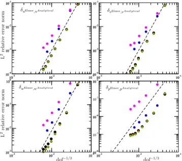
The Stokes solver is verified using the manufactured ana-lytical solution first proposed in Sargent and Fastook (2010) and subsequently modified and corrected in Leng et al. (2013). Here, we use exactly the same geometry and set of parameters as in Leng et al. (2013). All meshes are structured and defined by the number of elements inx,y andz direc-tions. The mesh discretisation is made to vary from a very coarse mesh (20×20×5, 10 584 degrees of freedom for the linear element) up to a fine mesh (160×160×40, 4 251 044 degrees of freedom). The modelled domain is the bumpy bed of ISMIP-HOM experiment A (Pattyn et al., 2008) with the 80 km length. For this geometry, the finer mesh does corre-spond to horizontal and mean vertical resolutions of 500 and 25 m, respectively. The convergence rate for the various el-ements and stabilisation methods is obtained as the slope of the L2 relative error norm function of the grid size refine-ment. TheL2relative error norm of two arbitrary vectorsu
andvis defined as
δu,v=
2|u−v|
|u+v|. (65)
10-3 10-2 10-1 10-4
10-3 10-2 10-1
10-3 10-2 10-1
10-4 10-3 10-2 10-1
10-3 10-2 10-1
10-4 10-3 10-2 10-1
10-3 10-2 10-1
10-4 10-3 10-2 10-1
10-3 10-2 10-1
10-3 10-2 10-1 100
10-3 10-2 10-1
10-3 10-2 10-1 100
10-3 10-2 10-1
10-6 10-5 10-4 10-3 10-2
10-3 10-2 10-1
10-6 10-4 10-2
L
2
re
la
t
iv
e
e
rro
r
n
o
rm
L
2
re
la
t
iv
e
e
rro
r
n
o
rm
dof−1/3
dof−1/3
δuElmer,uAnalytical δvElmer,vAnalytical
δwElmer,wAnalytical δpElmer,pAnalytical
Fig. 1.Results of the convergence tests:L2relative error norm
be-tween Elmer/Ice and analytical solutions for the 3 components of the velocity(u, v, w)and the pressure,p, as a function of the grid size (which is proportional to the inverse of the cubic root of the degrees of freedom) for Franca and Frey (1992) stabilisation with (black) 6-node wedge element, (red) 8-node hexahedron element and with (blue) 20-node hexahedron element; and for the residual free bubbles stabilisation (Baiocchi et al., 1993) with (green) 8-node hexahedron element and with (magenta) 20-node hexahedron ele-ment. The black dashed line indicates a rate of convergence of 3.
value expected (e.g. Ern and Guermond, 2004), especially for the linear element and pressure. Surprisingly, the same rate of convergence is obtained for linear and quadratic elements, and for a given discretisation the quality of the solution is even better using linear elements, so that the use of quadratic elements is not recommendable, at least in this particular ex-ample. For this application and the quadratic 20-node hexa-hedron element, the residual free bubbles method is found to be less accurate than the stabilisation method of Franca and Frey (1992).
7.2 Picard versus Newton linearisation
Picard and Newton schemes for the non-linear solution of the Stokes equations are compared by performing the ISMIP-HOM experiment A005 (Pattyn et al., 2008; Gagliardini and Zwinger, 2008) for two different initial conditions. The first one assumes null velocity and pressure, whereas the second initial condition is equal to the SIA solution for this problem. The switch from the Picard to the Newton iterative scheme is controlled by a criterion onδup,up+1, theL2relative error
norm, Eq. (65), between the previousp and currentp+1 velocity fields of the non-linear iteration loop. The same di-agnostic simulation is repeated for switch criteria of 10−6
0 10 20 30 40
10-7
10-6
10-5
10-4
10-3
10-2
10-1
100
L
2re
la
ti
ve
erro
r
n
orm
Iteration
Fig. 2.Evolution of theL2relative error norm between two
con-secutive solutions of the Stokes system,δup,up+1, as a function of
the non-linear iteration, for a switch criterion from the Picard to the Newton scheme of 10−6(Picard only, black curve), red 10−2, green 10−1, blue 1 and magenta 2 (Newton only), for the ISMIP-HOM experiment A005 with initial conditions (circle) assuming zero ve-locity and pressure and (triangle) estimated from the SIA solution. The colour of the dot-dashed lines indicates the value of the switch criterion of the corresponding colour curve.
(Picard only), 10−2, 10−1, 1 and 2 (Newton only). The non-linearity is assumed to be resolved whenδup,up+1<10
−6. The evolution ofδup,up+1as a function of the non-linear
it-eration indices is presented in Fig 2. As expected, the Newton scheme is quadratically convergent, while Picard converges only linearly (Paniconi and Putti, 1994). When the initial condition is null velocity and pressure, it takes 40 Picard it-erations to converge, whereas with Newton’s method alone, it requires only 10 iterations. Surprisingly, even if it takes less Picard iterations to converge for the SIA initial condi-tion, the convergence of the Newton solver is only obtained if Picard iterations are performed fromδup,up+1 <10
−1. This example shows that Newton’s method can diverge if the ini-tial condition is too far from the converged solution. A switch criterionδup,up+1 <10
−2is found to work in most cases and it reduces the non-linear iterations by a factor about 2. Be-cause the CPU consumption is almost proportional to the number of non-linear iterations performed within one time step, switching from Picard to Newton iterative schemes can reduce CPU time by the same factor.
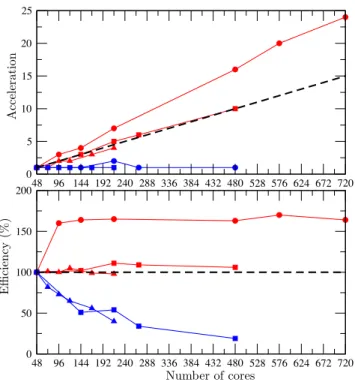
7.3 Elmer/Ice scalability
48 96 144 192 240 288 336 384 432 480 528 576 624 672 720 0
5 10 15 20 25
48 96 144 192 240 288 336 384 432 480 528 576 624 672 720 0
50 100 150 200
Ac
ce
le
ra
tio
n
Effi
ci
en
cy
(%
)
Number of cores
Fig. 3.Acceleration (top) and efficiency (bottom) for strong
scala-bility experiments using the block preconditioner for meshes with (red•) 2.400×10⁶nodes, (red) 1.142×10⁶nodes and (redN) 0.708×10⁶nodes, and the MUMPS solver for meshes with (blue ) 1.142×10⁶nodes and (blueN) 0.708×10⁶nodes. The dashed line indicates a theoretical efficiency of 100 %.
diagnostic Stokes solution is computed using the present-day Greenland geometry. The Greenland footprint is first meshed using regular triangle elements and then vertically extruded. Different meshes are constructed by varying the horizontal element size from 5 km to 10 km, but all have 20 vertical lay-ers. The size of the tested meshes varies from 708 000 up to 4 580 000 nodes. Temperature and basal drag are imposed using the same fields as in Gillet-Chaulet et al. (2012). New-ton iterations are used after the convergence criterion reaches 5×10⁻².
The results obtained for strong scalability, i.e. a constant problem size with different partitionings, and for weak scala-bility, i.e. a constant load per CPU using different mesh sizes, are presented in Figs. 3 and 4, respectively. If the elapsed time istnfor a number of partitionsn, then, for a strong
scal-ing test, the scalability of a solver can be characterised ei-ther by itsaccelerationtref/tnor itsefficiency(n/nref)tref/tn,
where ref stands for the reference simulation (often the one with the smallest mesh size). For a weak scaling test, the ac-celeration depicted in Fig. 4 is defined as(n/nref)tref/tn.
The weak scalability experiment uses a constant number of 4200 nodes per partition in combination with an increas-ing number of partitions from 168 up to 1092. Weak scala-bility is found to be greater than 60 % even for the largest test case. Efficiency greater than 100 % is obtained with the
0 200 400 600 800 1000
60 70 80 90 100
Effi
ci
en
cy
(%
)
Number of cores
Fig. 4.Efficiency for a weak scalability experiment using the block
preconditioner for an approximate number of nodes in all meshes of 4200 and meshes from 0.708×10⁶nodes up to 4.58×10⁶nodes.
new block preconditioned method for the strong scalability, whereas for a number of partitions greater than 100, MUMPS was always found to scale badly due to an increase of the re-quired memory. This new solution strategy using the block preconditioned solver clearly opens the door to applications one order of magnitude larger in mesh size than what we were able to achieve so far using a direct solver like MUMPS.
7.4 Inverse methods validation
We test the two inverse methods previously presented in a 2-D example resembling a calving glacier. As our objective is to validate the numerical implementation, we use a linear rheology for which the two inverse methods implemented are exact.
Our domain is 20 km long, the bed elevation is constant and equal to −900 m. The free-surface elevation decreases linearly from 200 m at x=0 km to 100 m at x=20 km. The free surface is stress-free, we prescribe an homogeneous Dirichlet condition of 50 m a−1for the horizontal velocity at
x=0 km, we apply a Neumann condition (hydrostatic sea pressure) atx=20 km, and we apply a linear sliding law and a non-penetration condition at the bedrock.
We generate a reference solution with
β=10−3(1.0+sin(2π x×2/L))MPa m−1a, (66)
η=10(1.5+sin(2π x×6/L))MPa a. (67) The surface velocities computed from this reference so-lution are then used as perfect synthetic observations (twin experiments).
10-10 10-8 10-6 10-4 10-2 100
0 100 200 300 400
10-6 10-4 10-2 100
|
dγ
Jo
|
/
|
dγ
Joi
n
i
|
Jo
/J
oin
i
Iterations
Fig. 5. Evolution as a function of the number of iterations of (top)
the cost function relative to the initial cost function and (bottom) the norm of the gradient vector relative to the initial gradient norm for the Robin (black curves) and control (red curves) inverse methods for the inversion ofβ(solid curve),Eη(x, y)(dashed curve) and
Eη(x, y, z)(dotted curve).
from the initial guessβi=10−3. The viscosityηis expressed
as η=Eηη0, and the optimisation is done on the viscos-ity enhancement factorEη with initial guessesEη=1 and
η0=15. It is possible a priori that several distributions ofEη,
especially in the vertical direction, can lead to the same sur-face velocities; therefore, we made it possible in the model to invertEη only in the horizontal plane(x, y)when using
vertically extruded meshes. The gradient ofJwith respect to
Eη at a given position(x, y)is then obtained as the vertical
sum of the nodal gradients at position(x, y).
To ensure thatβ andEη remain positive during the
opti-misation,βis expressed asβ=10α1 andE
ηis expressed as
Eη=α22. The optimisation is then done with respect to the
αi (i=1,2). The evolution of the cost function and norm of
the gradient obtained for each test is given in Fig. 5. Both the cost function and the gradient norm decrease and tend toward zero with the number of iterations.
The second step in the validation process is to verify the following approximation:
J (αi+hα′i)−J (αi)
h = ∇Jαi+o(1). (68)
For a given perturbationα′i, the left-hand-side term is eval-uated by computingJ (αi+hα′i)with the direct model for
several values of h, and the right-hand-side term is com-puted directly from the nodal gradients. This test is done
10-6 10-5 10-4 10-3 10-2 10-1 100 10-4
10-3 10-2 10-1 100
∆(
h
)
h
Fig. 6.Ratio1(h)obtained with the Robin (black curves) and
con-trol (red curves) inverse methods for perturbations of the enhance-ment factor to the viscosityEη(x, y).
for the initial conditions of the previous twin experiments. We also test the implementation of the Tikhonov regular-isation, Eq. (44), by choosing the cost function such as
J=R
Ŵb0.5(∂αi/∂x)
2dŴwhereα
i =1.0−9(1.0+sin(2.0π×
4x/L)).
For each solver, we use 10 random perturbation fieldsαi′
where each nodal value ofαi′ is a random number between
−50 % and 50 % of the mean value ofαi. The gradient
com-puted from the two inverse methods is verified using the ratio
1(h)defined as
1(h)=
(J (αi+hαi′)−J (αi))/ h− ∇Jαi
∇Jαi
. (69)
An example of the evolution of1(h)as a function of h is shown in Fig. 6 for the perturbation of the enhancement fac-tor to the viscosityEη(x, y). For both inverse methods and all
experiments, i.e. perturbation ofβ (not shown), Eη(x, y, z)
(not shown),Eη(x, y)(Fig. 6) and the Tikhonov
regularisa-tion (not shown), the ratio 1(h) is found to decrease as h
decreases and it reaches a value typically lower than 10 %. Such values are already satisfactory; nonetheless we could obtain even more accurate gradients by automatically deriv-ing the code itself.
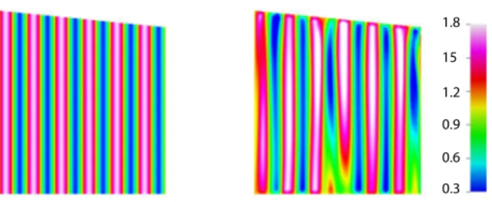
Figure 7 illustrates the difference of results obtained when inverting forEηonly in the horizontal plane or in the whole
ice volume. As can be seen, the two inferred fieldsEη(x, y)
andEη(x, y, z)are significantly different even if surface
1.8
0.3 0.6 0.9 1.2 15
Fig. 7. Comparison of the obtained inverted enhancement factor
field for the control method assuming only changes in a horizon-tal plane (Eη(x, y), left) or changes in all 3 directions (Eη(x, y, z),
right). The inverted fieldEη(x, y)in the left is virtually identical to
the one prescribed to obtain theobservedvelocities (Eq. 67).
8 Outlook
A number of the requisites for an ice sheet model as dis-cussed in the Introduction have already been implemented in Elmer/Ice, and especially those necessary to accurately de-scribe the flow of polar ice. Nevertheless, as for other ice sheet models, the physical processes at the boundaries and their coupling with the other components of the climate sys-tem can still be improved in the near future. This is the pre-requisite for running any forecast simulations of ice sheets, and not only sensitivity experiments based on more-or-less crude parameterisations that link changes in the atmosphere and the ocean to changes at the boundaries of the ice sheet. Our efforts in the near future will be dedicated to improv-ing the physical description of the ice/atmosphere, ice/ocean and ice/bedrock boundaries, as well as the models describing how the pertinent variables at these interfaces are distributed. For the basal boundary condition, numerical modelling (Schoof, 2010) or direct measurements (Sole et al., 2011) seem to indicate a very complex relation, most certainly non-linear, between changes in surface runoff and modulation of basal sliding. Two ingredients would then be required to fully account for the complexity of basal processes in rela-tion with changes in surface runoff: (i) a proper basal fricrela-tion law depending on the effective basal pressure (i.e. Eq. 22), and (ii) an associated hydrological model to describe the basal water pressure distribution. This hydrological model is currently under development and will be presented in de Fleurian et al. (2013).
Changes in the front position of marine-terminated glaciers seem to have a great influence on the upstream ice flow by modulating the buttressing force (Vieli and Nick, 2011). Determining the rate at which icebergs are calved for many different configurations remains an open question in glaciology. Submarine melting acting at the calving front of glaciers certainly increases calving rate by undercutting the ice (Rignot et al., 2010; O’Leary and Christoffersen, 2013). A general calving law, especially for 3-D configurations, still needs to be formulated (Benn et al., 2007). Better knowledge
of the stress distribution at the front of glaciers and of the submarine melting distribution, as well as a reliable ice dam-age model (e.g. Pralong, 2005; Jouvet et al., 2011), are the re-quired ingredients to describe calving at the front of marine-terminated glaciers. In Elmer/Ice, the already implemented ALE formulation for the free surface accounts for moving ice sheet margin boundaries. Because Elmer/Ice solves the full-Stokes system, all components of the stress field are known and can therefore be used to evaluate ice damage. Work is in progress to implement an ice damage rheological law follow-ing Pralong (2005) with the aim of usfollow-ing damage iso-surface to locate the calving surface and move accordingly the front surface.
Melting from beneath the ice shelves is certainly one the most important triggers of the observed recent ice stream ac-celerations (e.g. Payne et al., 2004; Dupont and Alley, 2005). Not only is the total amount of basal melting important, but also its spatial distribution (Gagliardini et al., 2010). For nu-merical and technical reasons, coupling an ocean model with an ice sheet model is still a challenging issue. An interme-diate approach we would like to explore as a preliminary step towards a complete coupling with an ocean model is the implementation within Elmer/Ice of a plume-type model (Holland and Feltham, 2006).
9 Conclusions