A Competitive Facility Location Problem on a
Network with Fuzzy Random Weights
Takeshi Uno, Hideki Katagiri,
Member, IAENG,
and Kosuke Kato
Abstract—This paper focuses on a new Stackelberg location problem on a network with demands whose weights are given uncertainly and vaguely. By representing them as fuzzy random variables, the optimal location problem can be formulated as a fuzzy random programming problem for finding Stackelberg equilibrium. By using both their�-level sets for fuzziness and
their satisfaction level for a given probability for randomness, it can be reformulated as a version of conventional Stackelberg location problem on the network. Theorems for its complexity are shown based upon the characteristics of the facility location.
Index Terms—facility location, competitiveness, Stackelberg equilibrium, fuzzy random variables.
I. INTRODUCTION
A. Former Studies of Stackelberg Location Problems
C
OMPETITIVE facility location problem (CFLP) is one of optimal location problems for commercial facilities, e.g. shops and stores, and an objective of most CFLPs is to obtain as many buying powers (BPs) from customers as possible. Mathematical studies on the CFLPs were origi-nated by Hotelling [7]. He considered the CFLP under the conditions that (i) customers are uniformly distributed on a line segment, (ii) each of decision makers (DMs) will locate her/his own facility on the line segment that there are no facilities, and (iii) all customers only use the nearest facility. Then, his CFLP can be represented as an optimal location problem for finding Nash equilibrium, called Nash location problem (NLP). As an extension of Hotelling’s NLP, Wendell and McKelvey [23] assumed that there exist customers on a finite number of points, called demand points (DPs), and considered an NLP on a network whose vertices are DPs.On the other hand, based upon the NLP by Wendell and McKelvey [23], Hakimi [5] considered the CFLP with two types of DMs; the upper DM, who first locates her/his facil-ities, and the lower DM, who next locates her/his facilities. Then, his CFLP for the upper DM can be represented as an optimal location problem for finding Stackelberg equilib-rium, called Stackelberg location problem (SLP). For details of Hakimi’s SLP and their applications, the readers can refer to the book of Miller et al. [11]. As an extension of Hakimi’s SLP, SLPs on a plane are considered by Drezner [3], Uno et al. [17], [18], etc. Another type of SLP based on maximal covering is considered by Plastria and Vanhaverbeke [13].
In the above studies of CFLPs, weights of demands for facilities are represented as definite values. We consider some
Manuscript received May 14, 2011; revised May 14, 2011.
T. Uno is with Institute of Socio-Arts and Sciences, the University of Tokushima, 1-1, Minamijosanjima-cho, Tokushima-shi, Tokushima, 770-8502 JAPAN. e-mail: [email protected]
H. Katagiri is with Hiroshima University. e-mail: [email protected]
K. Kato is with Hiroshima Institute of Technology. e-mail: [email protected]
uncertainty and vagueness included in the weights. For the uncertainty, facility location model with random weights in a noncompetitive environment is considered by Wagnera et al. [21]; for the details of location models with random weights, the reader can refer to the study of Berman and Krass [2]. For CFLPs with random weights, Shiode and Drezner [15] considered an SLP on a tree network, and Uno et al. [17] considered a CFLP on a plane. On the other hand, for the vagueness, facility location model with fuzziness in a noncompetitive environment is considered by Moreno P´erez et al. [12], which represented the weights as fuzzy numbers proposed by Dubois and Prade [4]. Recently, the decision-making problems in environments including both uncertainty and vagueness are studied. Kwakernaak [10] proposed the fuzzy random variable representing both fuzziness and ran-domness. For the details of fuzzy random variable, the reader can refer to the book of Kruse and Meyer [9]. Fuzzy random programming and its distribution problems are considered by Wang and Qiao [22] and Qiao and Wang [14]. For the recent studies of fuzzy random programming problems, Katagiri et al. [8] considered multiobjective fuzzy random linear programming, and Ammar [1] considered fuzzy random multiobjective quadratic programming. Uno et al. [18], [20] considered CFLPs with weights represented as fuzzy random numbers, and Uno et al. [19] considered SLPs with demands on a tree network, whose sites are represented as fuzzy random variables.
B. An Outline of Our study
In this paper, we propose a new SLP on a network by introducing fuzzy random weights. Then, we can formulate the SLP by representing the randomness as scenarios for each weight. For solving the SLP, we first transform it to an SLP with random weights by using the definition of �-level sets for fuzziness. Next, we use the satisfaction level for a given probability for randomness. Then, we can reformulate it to a version of conventional SLP on a network with nonfuzzy and nonrandom weights, and can show theorems for its complexity based upon the characteristics of the facility location.
The remaining structure of this article is organized as fol-lows: The next section devotes to introducing the definition of fuzzy random variables. In Section 3, we formulate the SLP on a tree network with weights including uncertainly and vaguely as an SLP with fuzzy random variables. By using
�-level sets and satisfaction level for a given probability, we reformulate it the problem to a version of conventional SLP on a tree network in Section 4. Section 5 shows theorems for its complexity based upon the characteristics of the facility location on tree networks. We extend the results of SLP on tree networks to that on general networks in Section 6.
Engineering Letters, 19:2, EL_19_2_08
(Advance online publication: 24 May 2011)
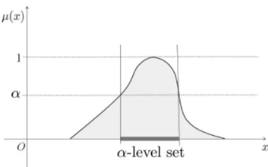
Fig. 1. An Example of Fuzzy Numbers and its�-Level Set
Fig. 2. An Example of Fuzzy Random Variables
Finally, conclusions and future studies are summarized in Section 7.
II. FUZZYRANDOMVARIABLE
Let �˜ be fuzzy number and ��˜ : R → [0,1] be membership function of �˜, where R is the set of real
numbers. For �∈(0,1], the �-level set of�˜ is represented as the following equation:
˜
��≡ {�∣��˜(�)≥�} (1) Fig. 1 illustrates an example of fuzzy numbers and its�-level set.
In this paper, we use the following definition of fuzzy random variable, suggested by Kruse and Meyer [9]:
Definition 2.1: Let (Ω, �, �) be a probability space, where Ω, �, and � are a sample space, �-algebra, and a probability measure function, respectively. Let ℱ(R) be
the set of fuzzy numbers with compact supports, and Ξ a measurable mappingΩ→ ℱ(R). ThenΞis a fuzzy random
variable if and only if given�∈Ω, its�-level setΞ�(�)is a random interval for any �∈(0,1].
Fig. 2 illustrates an example of fuzzy random variables for representing BP per day for weather, whose randomness is represented by weather and whose fuzziness is included in the BP for each case of weather.
III. FORMULATION OFSLPWITHFUZZYRANDOM QUANTITYDEMANDED
We consider the SLP on a weighted tree � = (�, �), which is a simple graph, where � and � are the sets of
Fig. 3. An Example of Tree Networks of the SLP
vertices and edges, respectively. For each vertex � ∈ �
and edge � ∈ �, we associate weights �(�), �(�) ≥ 0, respectively, where �(�) means the BP of the weight on
� for facilities and�(�)the length of�. Fig. 3 illustrates an example of tree networks of the SLP.
In the tree�, we consider the case that each�(�),�∈�
is given as the following fuzzy random variable:
∙ Its randomness is given by � scenarios, whose
proba-bilities are denoted by�1, �2, . . . , �� >0.
∙ For each scenario�= 1,2, . . . , �, its fuzziness is given
as fuzzy number ��(�) ∈ ℱ(R) whose membership function is denoted by���(�)(�), where���(�)(�) = 0
for any � < 0 and its �-level set is closed for any
�∈(0,1].
An example of fuzzy random weights is shown in Fig. 2. Let�and� be the given numbers of facilities located by the upper and lower DMs, respectively. Let�1, �2, . . . , ��∈
� be the sites of the upper DM’s facilities and �� = {�1, �2, . . . , ��}. Similarly, let �1, �2, . . . , �� ∈ � be the sites of the lower DM’s facilities and��={�1, �2, . . . , ��}. We assume that each of customers only use the nearest facility, and the facility providing some service to customers on�can obtains�(�)from�∈�. If two or more facilities are the same distances to a customer, one of the upper DM’s facilities can obtain her/his BP.
Let �� �(��, ��) be the sum of obtaining BPs of the upper DM’s facilities from the customers. Note that
�� �(��, ��) is represented as a fuzzy random number. The objective of each DM is defined to maximize her/his obtaining BPs. Since the sum of obtaining BPs of all facilities is constant, the objective of the lower DM can be represented as minimizing the sum of the upper DM’s obtaining BPs. For given location �� ∈ �� = � × ⋅ ⋅ ⋅ ×�, the optimal location problem for the lower DM, called(��∣�)-medianoid problem, can be formulated as follows:
minimize �� �(��, ��) subject to ��∈��.
}
(2)
Let �∗
�(��) be the optimal solution of (��∣�)-medianoid problem. Then, the proposed SLP, called(�∣�)-centroid prob-lem, can be formulated as follows:
maximize �� �(��, ��∗(��)) subject to �� ∈��.
}
(3)
Engineering Letters, 19:2, EL_19_2_08
(Advance online publication: 24 May 2011)
IV. REFORMULATION TO A VERSION OF CONVENTIONAL SLP
For (2) and (3), their objective functions values are repre-sented as fuzzy random numbers. Then, we need to define an order between fuzzy random numbers. In this paper, we reformulate (2) and (3) to a version of conventional medianoid and centroid problems, respectively.
We first transform (2) and (3) to the following stochastic programming problems by using the �-level set (1). For a given�∈(0,1], we assume that the lower DM can decide the variable in each of�-level sets for minimizing the upper DM’s objective function value. Then, we can represent the lower DM’s objective function value as
��
�(��, ��) = min{(�� �(��, ��))�} (4) Because ��
�(��, ��) is a random value, (2) can be trans-formed as the following stochastic programming problem:
minimize ��
�(��, ��) subject to ��∈��.
}
(5)
Let��
� (��)be the optimal solution of (5). Then, (3) can be reformulated as follows:
maximize ��
�(��, ���(��)) subject to �� ∈��.
}
(6)
Next, by using the satisfaction level for a given probability for their randomness, we reformulate (5) and (6) to determin-istic programming problems. For probability 1/2 < � <1 given by the upper DM, we use the following constraint for the lower DM suggested by Shiode and Drezner [15]:
� �{���(��, ��)≤�} ≥�, (7) where �means a satisfaction level for the upper DM. Then, (5) can be reformulated as follows:
minimize �
subject to � �{��
�(��, ��)≤�} ≥�,
��∈��.
⎫ ⎬
⎭
(8)
Let ��(�,�)(��) be the optimal solution of (8). Contrary to (7), the upper DM would like to increase her/his satisfaction level for a given probability �. Then, the constraint for the upper DM can be represented as
� �{��
�(��, ��(�,�)(��))≥�} ≥�. (9) Hence (6) can be reformulated as follows:
maximize �
subject to � �{��
�(��, ��(�,�)(��))≥�} ≥�,
�� ∈��.
⎫ ⎬
⎭
(10)
Because (10) include constraint (9), (10) is not a conven-tional SLP but a version of convenconven-tional SLP.
V. COMPLEXITY AND SOLUTION METHOD OF THESLP For cases that the tree network does not include any fuzzy random weights, (2) and (3) can be reduced to conventional medianoid and centroid problems, respectively, which are NP-hard if �≥2 proven by Hakimi [6] and Spoerhase and Wirth [16]. Therefore, the following theorems are apparently satisfied:
Lemma 5.1: For any��∈�� with�≥2, (8) is NP-hard.
Theorem 5.2: For any�≥2, (10) is NP-hard.
Then, we consider (8) and (10) for the case � = 1. We first show the following two lemmas for solving (8).
Lemma 5.3: If �1 is on any vertex � ∈�, then one of
��(�,�)(�1) can be given by locating all � facilities on the opposite vertices of the edges adjacent to�.
Proof:Note that any tree can be cut to several trees by removing any one non-leaf vertex or edge. A lower DM’s facility can obtain all BPs on the tree that is cut at a point between her/his facility and the upper DM’s facility and includes her/his facility. The best location of the lower DM is clearly so as not to put any nodes between her/his facilities and�. This means that one of��(�,�)(�1)can be represented by locating her/his�facilities on the set of the above points.
Similarly to the above proof, the following lemma can be shown.
Lemma 5.4: If�1 is on point� in any edge�∈�, then one of ��(�,�)(�1) is to locate facilities on both vertices adjacent to�if�≥2, or either vertex if�= 1.
Next we consider (10) for the case�= 1.
Theorem 5.5: The optimal solution for (10) with�= 1is to locate it on one of the vertices.
Proof: We show the proof of the theorem by the reduction to absurdity. We assume the upper DM locates on any edge � ∈ �. If � ≤ 2, the lower DM can reduce the objective function value of (10) to zero by locating her/his two facilities at both points adjacent to�. On the other hand, if � = 1, the optimal location of the lower DM can be found by Lemma 5.4 and its candidates are only two points. Whichever is optimal for the lower DM, the upper DM can obtain more BPs by locating at the vertex than that on �. These contradict the optimality of (10).
Note that we can show the proofs of Lemmas 5.3, 5.4, and Theorem 5.5 in a similar way of those of the conventional medianoid and centroid problems.
Finally, we consider the complexity for (10) for the case
�= 1. From Theorem 5.5, we can find an optimal solution of (10) by examining all vertices. For the case that the upper DM locates her/his one facility on each vertex � ∈ �, we need to solve (8). From Lemma 5.3, (8) for each location can be solved by examining all the opposite vertices of the edges adjacent to �. Let ∣�∣ denote the number of edges. Then, for all locations of the upper DM, the total number of the examination is2∣�∣. This means that (10) can be solved in polynomial time.
VI. EXTENSION OF THESLPTO THAT ON A GENERAL NETWORK
In this section, we consider the SLP on a general network
�, that is, the following problems: minimize �
subject to � �{��
�(��, ��)≤�} ≥�,
��∈��,
⎫ ⎬
⎭
(11)
Engineering Letters, 19:2, EL_19_2_08
(Advance online publication: 24 May 2011)
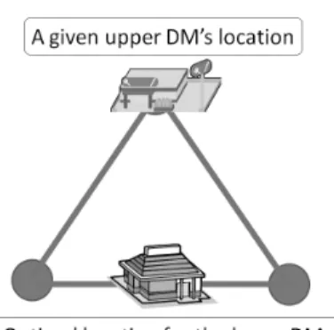
Fig. 4. A Difficulty of the SLP on the general network
and
maximize �
subject to � �{�� �(��, �
(�,�)
� (��))≥�} ≥�,
�� ∈��,
⎫ ⎬
⎭
(12)
where ��(�,�)(��)is an optimal solution of (11). Note that (11) and (12) are usually difficult to solve than (8) and (10). We show such a difficulty by illustrating a simple example of the SLP.
In Fig. 4, we consider the SLP that each of both DMs locates only one facility on the triangle network, three of whose nodes has the same BPs, and three of whose edges has the same length. We consider the case that the upper DM locates her/his facility on one of the nodes. If the lower DM also locates her/his facility on another node, she/he only obtain BPs from one node. However, if she/he locates it on the edge not adjacent to the node with the upper DM’s facility, she/he can obtain BPs from two nodes. This means that Lemmas 5.3 and 5.4 are not satisfied, and then Theorem 5.5 is not satisfied for the SLP on the general network.
However, for cases that the general network does not include any fuzzy random weights, (11) and (12) can be reduced to conventional medianoid and centroid problems, respectively, both of whose complexities are shown by Hakimi [5]. From the discussion of the previous section, the following theorems of (11) and (12) can be shown in a similar way of those of conventional medianoid and centroid problems.
Lemma 6.1: For any �� ∈ �� with � ≥ 2, (11) is NP-hard.
Theorem 6.2: For any�≥2, (12) is NP-hard.
Lemma 6.3: For any �� ∈ �� with � = 2, (11) can be solved in polynomial time.
Theorem 6.4: For any � = 1, (12) can be solved in polynomial time.
VII. CONCLUSIONS AND FUTURE STUDIES In this paper, we have proposed a new Stackelberg location problem on a network with weights including uncertainly and vaguely. For formulating the Stackelberg location problem with the fuzzy random variables, by using their�-level sets and satisfaction level, we have reformulated as a version of
conventional Stackelberg location problem on a network. Its complexity have been shown based upon the characteristics of the facility location.
This paper shows that (8), (10), (11), and (12) with�≥2 are NP-hard. To propose an efficient solution method for these problems are an important future study.
REFERENCES
[1] E. E. Ammar, “On Fuzzy Random Multiobjective Quadratic Program-ming,”European Journal of Operational Research, vol.193, pp. 329-340, Mar. 2009.
[2] O. Berman, K. Krass, “Facility Location with Stochastic Demands and Congestion,” inZ. Drezner, H. W. Hamacher (eds.) Facility Location: Application and Theory, pp. 329-372, Springer, Berlin, 2001. [3] Z. Drezner, “Competitive Location Strategies for Two Facilities,”
Re-gional Science and Urban Economics, vol. 12, pp. 485-493, Nov. 1982. [4] D. Dubois, H. Prade, “Operations on Fuzzy Numbers,”Int. Journal
Systems Science, vol. 9, pp. 613-626, Jun. 1978.
[5] S. L. Hakimi, “On Locating New Facilities in a Competitive Environ-ment,”European Journal of Operational Research, vol. 12, pp. 29-35, Jan. 1983.
[6] S. L. Hakimi, “Locations with Spatial Interactions: Competitive Loca-tions and Games,” inP. B. Mirchandani, R. L. Francis (eds.), Discrete Location Theory, Series in Discrete Mathematics and Optimization, pp. 439-478. Wiley-Interscience, 1990.
[7] H. Hotelling, “Stability in Competition,”The Economic Journal, vol. 30, pp. 41-57, Mar. 1929.
[8] H. Katagiri, M. Sakawa, K. Kato, I. Nishizaki, “Interactive Multiobjec-tive Fuzzy Random Linear Programming: Maximization of Possibility and Probability,”European Journal of Operational Research, vol. 188, pp. 530-539, Jul. 2008.
[9] R. Kruse, K. D. Meyer, Statistics with Vague Data, D. Riedel Publishing Company, Dordrecht, 1987.
[10] H. Kwakernaak, “Fuzzy Random Variables-I. Definitions and Theo-rems,”Information Sciences, vol. 15, pp. 1-29, Jul. 1978.
[11] T. C. Miller, T. L. Friesz, R. L. Tobin,Equilibrium Facility Location on Networks, Springer Verlag, Berlin, 1996.
[12] J. A. Moreno P´erez, , L. Marcos Moreno Vega, J. L. Verdegay, “Fuzzy Location Problems on Networks,”Fuzzy Sets and Systems, vol. 142, pp. 393-405, Mar. 2004.
[13] F. Plastria, L. Vanhaverbeke, “Discrete Models for Competitive Loca-tion with Foresight,”Computers & Operations Research, vol. 35, pp. 683-700, Feb. 2008.
[14] Z. Qiao, G. Wang, “On Solutions and Distribution Problems of the Linear Programming with Fuzzy Random Variable Coefficients,”Fuzzy Sets and Systems, vol. 58, pp. 120-155, Sep. 1993.
[15] S. Shiode, Z. Drezner, “A Competitive Facility Location Problem on a Tree Network with Stochastic Weights,” European Journal of Operational Research, vol. 149, pp. 47-52, Aug. 2003.
[16] J. Spoerhase, H. C. Wirth, “(�, �)-Centroid Problems on Paths and
Trees,”Theoretical Computer Science, vol. 410, pp. 5128-5137, Nov. 2003.
[17] T. Uno, H. Katagiri, K. Kato, “Competitive Facility Location with Random Demands,”IAENG Transactions on Engineering Technologies, vol. 3, pp. 83-93, America Institute of Physics, 2009.
[18] T. Uno, H. Katagiri, K. Kato, “A Facility Location for Fuzzy Random Demands in a Competitive Environment,”IAENG International Journal of Applied Mathematics, vol. 40, no. 3, pp. 172-177, Aug. 2010. [19] T. Uno, H. Katagiri, K. Kato, “Competitive Facility Location with
Fuzzy Random Demands,”IAENG Transactions on Engineering Tech-nologies, vol. 5, pp. 99-108, America Institute of Physics, 2010. [20] T. Uno, H. Katagiri, K. Kato, “Stackelberg Location on a Tree
Network with Fuzzy Random Quantities Demanded,” Lecture Notes in Engineering and Computer Science: Proceedings of The International MultiConference of Engineers and Computer Scientists 2011, IMECS 2011, 16-18 March, 2011, Hong Kong, pp. 1395-1398.
[21] M. R. Wagnera, J. Bhaduryb, S. Penga, “Risk Management in Unca-pacitated Facility Location Models with Random Demands,”Computers & Operations Research, vol. 36, pp. 1002-1011, Apr. 2009.
[22] G. Y. Wang, Z. Qiao, “Linear Programming with Fuzzy Random Variable Coefficients,”Fuzzy Sets and Systems, vol. 57, pp. 295-311, Aug. 1993.
[23] R. E. Wendell, R. D. McKelvey, “New Perspective in Competitive Location Theory,”European Journal of Operational Research, vol. 6, pp. 174-182, Feb. 1981.