Evaluation of MERIS products from Baltic Sea coastal waters rich in CDOM

www.ocean-sci.net/10/377/2014/ doi:10.5194/os-10-377-2014

© Author(s) 2014. CC Attribution 3.0 License.

Evaluation of MERIS products from Baltic Sea coastal waters rich

in CDOM

J. M. Beltrán-Abaunza1, S. Kratzer1, and C. Brockmann2

1_{Department of Ecology, Environment and Plant Sciences, Stockholm University 106 91, Stockholm, Sweden} 2_{Brockmann Consult GmbH, Max-Planck-Str. 2, 21502 Geesthacht, Germany}

Correspondence to:J. M. Beltrán-Abaunza (jose.beltran@su.se)

Received: 26 September 2013 – Published in Ocean Sci. Discuss.: 28 November 2013 Revised: 20 March 2014 – Accepted: 2 April 2014 – Published: 23 May 2014

Abstract. In this study, retrievals of the medium resolu-tion imaging spectrometer (MERIS) reflectances and water quality products using four different coastal processing algo-rithms freely available are assessed by comparison against sea-truthing data. The study is based on a pair-wise com-parison using processor-dependent quality flags for the trieval of valid common macro-pixels. This assessment is re-quired in order to ensure the reliability of monitoring sys-tems based on MERIS data, such as the Swedish coastal and lake monitoring system (http://vattenkvalitet.se). The results show that the pre-processing with the Improved Contrast be-tween Ocean and Land (ICOL) processor, correcting for ad-jacency effects, improves the retrieval of spectral reflectance for all processors. Therefore, it is recommended that the ICOL processor should be applied when Baltic coastal wa-ters are investigated. Chlorophyll was retrieved best using the FUB (Free University of Berlin) processing algorithm, although overestimations in the range 18–26.5 %, dependent on the compared pairs, were obtained. At low chlorophyll concentrations (<2.5 mg m−3), data dispersion dominated in the retrievals with the MEGS (MERIS ground segment pro-cessor) processor. The lowest bias and data dispersion were obtained with MEGS for suspended particulate matter, for which overestimations in the range of 8–16 % were found. Only the FUB retrieved CDOM (coloured dissolved organic matter) correlate with in situ values. However, a large sys-tematic underestimation appears in the estimates that nev-ertheless may be corrected for by using a local correction factor. The MEGS has the potential to be used as an opera-tional processing algorithm for the Himmerfjärden bay and adjacent areas, but it requires further improvement of the

atmospheric correction for the blue bands and better defini-tion at relatively low chlorophyll concentradefini-tions in the pres-ence of high CDOM attenuation.

1 Introduction

specifically from MERIS measurement.The dominance of aCDOM in the attenuation of light continues to be a chal-lenge for chlorophylla retrieval algorithms in ocean colour remote sensing (Carder et al., 1991; Nelson and Siegel, 2013).

In coastal waters, suspended sediment and dissolved or-ganic matter usually do not co-vary with the chlorophyll a concentration (Morel and Prieur, 1977). Different combina-tions and concentracombina-tions of optical constituents may result in the same spectral reflectance signature measured by the sen-sors, making it difficult to interpret. This, in turn, may hinder accurate retrieval of absorption and scattering properties (i.e. inherent optical properties, IOPs) and subsequent retrieval of concentrations of optical water constituents.

Elaborate methods are required to derive the concentra-tions of optical variables accurately from space, e.g. matrix or neural network inversion (IOCCG, 2010). Different algo-rithms have been developed for this task which have been validated against in situ measurements and inter-compared. Of those, the most common coastal processors that are dis-tributed freely were used in this study: the standard MEGS processor (Case-2 water processing branch), the FUB/WeW processor developed by the Free University Berlin, here ferred to as FUB (Schroeder et al., 2007a, b), the Case-2 re-gional processor C2R (Doerffer and Schiller, 2007) and the boreal water processor (BOREAL) (Doerffer and Schiller, 2008). Each of the above processors (including the Case-2 branch of MEGS) use a multiple nonlinear regression method, i.e. a neural network, that includes simulations of radiative transfer models to derive the light propagation through the water and the atmosphere linked with bio-optical models. It must be noted that the FUB processor resolves the water products directly from top-of-atmosphere radiance, whereas the other three processors first derive the level 2 re-flectance. The latter is then used to derive IOPs (absorption and scattering), which are subsequently used to derive the level 2 water products.

The combined use of satellites and in situ observations can maximize the benefits of ocean colour observations (Gregg and Conkright, 2001). Currently, only three satellite ocean colour sensors have about 10 years of global coverage of data, i.e. SeaWiFS (1997–2011, NASA), MODIS (1999– ongoing, NASA) and MERIS (2002–2012, ESA). MERIS was especially adapted for coastal applications. It had high spatial resolution (290 m×260 m) and spectral resolution (15 spectral channels in the visible and near-infrared region), compared to the other sensors (Doerffer et al., 1999; Euro-pean Space Agency, 2011). However, contact with the EN-VISAT spacecraft was lost in April 2012, and hence trans-mission of MERIS data was no longer possible. The cur-rent focus of the ENVISAT mission is to encourage data exploitation of the 10-year satellite data archive and to up-grade and validate image processing algorithms in order to derive the geophysical products (level 2 processing) accu-rately (Laur, 2012). This will lead to improved algorithms

for the operational follow-up mission of MERIS, Sentinel-3 (the launch is planned in November 2014), which will carry the Ocean Land Colour Instrument (OLCI) that has improved characteristics compared to MERIS; e.g. a spectral resolution of 21 wavelength bands in the range 400–1020 nm.

The small number of in situ data available in optically complex waters to train “global” algorithms, supports the requirement for “regional” algorithms as a complement (Kajiyama et al., 2013). In the study of Zibordi et al. (2013), the standard products of 3rd reprocessing MERIS data sets were evaluated for European seas. Their study reinforces the need to substantially increase the number of highly accurate and globally distributed in situ measurements to adequately address regional uncertainties that affect ocean colour data products. On a regional level, Kratzer et al. (2008) showed that the FUB processor was best for retrieving level 2 prod-ucts from the Himmerfjärden area, including the NW Baltic Proper. The FUB has also been applied successfully in other areas of the Baltic Sea (Ohde et al., 2007; Vaiˇci¯ut˙e et al., 2012). Kratzer and Vinterhav (2010) showed that the retrieval of level 2 products over Swedish coastal waters was im-proved by using a combination of the Imim-proved Contrast be-tween Ocean and Land (ICOL) processor (Santer and Zagol-ski, 2007, 2009), correcting for adjacency effects, and the FUB processor. An independent end-user survey also tested the results of different processing schemes in coastal and lake areas (Philipson et al., 2009). All end-users confirmed that the images that had been processed with ICOL and FUB represented best the ranges of water quality parameters for the respective water body (Swedish great lakes and Himmer-fjärden area) and season. The processing chain ICOL-FUB was therefore applied to the operational monitoring system (http://vattenkvalitet.se) for the Swedish great lakes and the coastal areas.

processing recommendations for the current monitoring sys-tem, based on MERIS data 3rd reprocessing, to identify the advantage of the different MERIS processors for the retrieval of water quality parameters in the Baltic Sea and, further-more, to make recommendations for future satellite missions such as Sentinel-3, which is planned to be launched by ESA at the end of 2014.

2 Data and methods 2.1 Study area

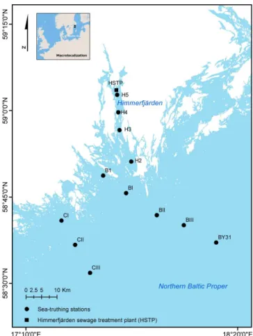
The region of interest is on the northwestern coast of the Northern Baltic Proper (Fig. 1), south of Stockholm Archipelago, including Himmerfjärden bay and its adja-cent areas, top-left latitude and longitude (60◦_{N, 17}◦_E)

and bottom-right coordinates (58◦_{N, 19}◦_{E). This region is}

a brackish marine ecosystem (Elmgren, 2001). The influ-ence of tides is negligible in most of the Baltic Sea, therefore the main circulation is driven by the surface wind speed and changes in atmospheric pressure (Leppèaranta and Myrberg, 2009). The Baltic Sea and Himmerfjärden are optically dom-inated by CDOM absorption (Kutser et al., 2009; Kratzer and Tett, 2009).

Himmerfjärden bay follows a regular phenology of phy-toplankton blooms that occur in the Baltic Sea during spring and summer. The summer blooms are of special environmental and health interest because they are domi-nated by the potentially toxic nitrogen-fixing filamentous Cyanobacteria,Nodularia spumigenaand non-toxic Aphani-zomenom sp. The chlorophylla (Chla) concentrations that can be observed within Himmerfjärden range from 1 up to 18 mg m−3_{, with higher values during the spring bloom. The} suspended particulate matter (SPM) load ranges from 0.5 up to 2.7 g m−3 with decreasing values towards the open sea (Kratzer and Tett, 2009). The absorption of CDOM (g440) in Himmerfjärden ranges from 0.39 up to 1.27 m−1, and in the open sea from about 0.3 to 0.5 m−1. The Himmerfjärden region has a local catchment area of 536 km2receiving a mi-nor freshwater outflow from Lake Mälaren (Franzén et al., 2011). Located within the Himmerfjärden bay (Fig. 1) is the third largest sewage treatment plant in the Stockholm region. From 2007 to 2010 an adaptive management experiment was carried out in the Himmerfjärden sewage treatment plant (HSTP) to study the effects of nitrogen release on eutrophica-tion and the development of cyanobacterial blooms. The ex-periment entailed effluent release without nitrogen treatment during 2007–2008, and with full-capacity nitrogen treatment during 2009–2010.

Figure 1. Himmerfjärden is the region of interest, where sea-truthing campaigns were performed in 2008 and 2010. See Table 1 for campaign dates and time of the satellite overpasses.

2.2 Sea-truthing data 2.2.1 Water samples

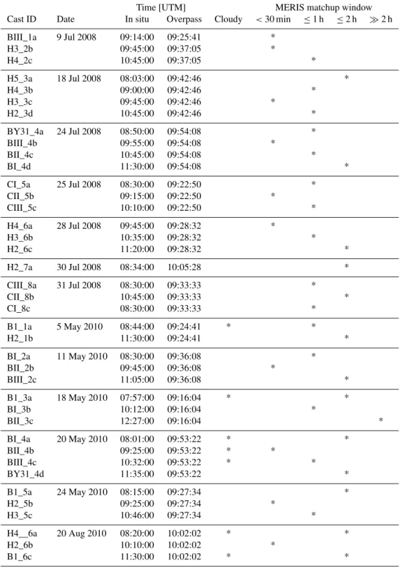
Table 1.Matchup timetable. Note: Cast ID refers to the site, number of transect, and sampling ID.

Time [UTM] MERIS matchup window

Cast ID Date In situ Overpass Cloudy <30 min ≤1 h ≤2 h ≫2 h

BIII_1a 9 Jul 2008 09:14:00 09:25:41 *

H3_2b 09:45:00 09:37:05 *

H4_2c 10:45:00 09:37:05 *

H5_3a 18 Jul 2008 08:03:00 09:42:46 *

H4_3b 09:00:00 09:42:46 *

H3_3c 09:45:00 09:42:46 *

H2_3d 10:45:00 09:42:46 *

BY31_4a 24 Jul 2008 08:50:00 09:54:08 *

BIII_4b 09:55:00 09:54:08 *

BII_4c 10:45:00 09:54:08 *

BI_4d 11:30:00 09:54:08 *

CI_5a 25 Jul 2008 08:30:00 09:22:50 *

CII_5b 09:15:00 09:22:50 *

CIII_5c 10:10:00 09:22:50 *

H4_6a 28 Jul 2008 09:45:00 09:28:32 *

H3_6b 10:35:00 09:28:32 *

H2_6c 11:20:00 09:28:32 *

H2_7a 30 Jul 2008 08:34:00 10:05:28 *

CIII_8a 31 Jul 2008 08:30:00 09:33:33 *

CII_8b 10:45:00 09:33:33 *

CI_8c 08:30:00 09:33:33 *

B1_1a 5 May 2010 08:44:00 09:24:41 * *

H2_1b 11:30:00 09:24:41 *

BI_2a 11 May 2010 08:30:00 09:36:08 *

BII_2b 09:45:00 09:36:08 *

BIII_2c 11:05:00 09:36:08 *

B1_3a 18 May 2010 07:57:00 09:16:04 * *

BI_3b 10:12:00 09:16:04 *

BII_3c 12:27:00 09:16:04 *

BI_4a 20 May 2010 08:01:00 09:53:22 * *

BII_4b 09:25:00 09:53:22 * *

BIII_4c 10:32:00 09:53:22 * *

BY31_4d 11:35:00 09:53:22 *

B1_5a 24 May 2010 08:15:00 09:27:34 *

H2_5b 09:25:00 09:27:34 *

H3_5c 10:46:00 09:27:34 *

H4__6a 20 Aug 2010 08:20:00 10:02:02 * *

H2_6b 10:10:00 10:02:02 *

B1_6c 11:30:00 10:02:02 * *

Concentrations of organic and inorganic SPM were mea-sured by the gravimetric method (Strickland and Parsons, 1972). This method has an error of 10 % to derive total SPM in summer from surface water samples in the Baltic Sea (Kratzer, 2000). For the determination of aCDOM, the water was filtered through 0.2 µm membrane filters and measured

(Chl a), the trichromatic method was applied (Jeffrey and Humphrey, 1975; Parsons et al., 1984). The samples were filtered through GF/F filters and kept in liquid nitrogen un-til they were analysed. They were then extracted into 90 % acetone using sonication. The trichromatic method has an error of 7 % when deriving Chla from the Baltic Sea. The percentage error of the in situ values (i.e. SPM, Chla) cor-respond to the coefficient of variation (i.e. standard devia-tion/mean), using all the available samples from different bottles (Kratzer, 2000). During 2002, an international chloro-phyll inter-calibration exercise was coordinated by the Nor-wegian Institute of Water Research (NIVA) for the European MERIS Validation Team (MVT) (Sørensen et al., 2007). The results of the MVT inter-calibration showed that the spec-trophotometric Chlameasurements of natural water samples by the marine remote sensing group from Stockholm Uni-versity were within 8.6 % of the median value of the interna-tional group. In previous tests the method to derive aCDOM had shown much less variability between replicates from dif-ferent bottles (Kratzer, 2000), than for SPM and Chla, and in this study it is assumed to be well below 5 %.

2.2.2 Field radiometry

The Tethered Attenuation Coefficient Chain-Sensor (TACCS, manufactured by Satlantic Inc., Canada) is an in-water radiometer deployed on a floating buoy. The TACCS has an in-water up-welling radiance sensor Lu (λ) with a full-angle field of view (FAFOV) of 20◦ _{at nominal}

depth 0.5 m. The Lu sensor has seven channels matching the MERIS bands centred at 412, 443, 490, 510, 560, 620 and 665 nm. The TACCS includes an in-air downward irradiance sensor Ed centred at 443, 490 and 670 nm. The TACCS also includes an in-water chain of Ed (λ=490 nm) at the nominal depths of 2, 4, 6 and 8 m. All sensors have a 10 nm bandwidth. TACCS measurements were logged in 3 min intervals at an acquisition rate of 0.5 Hz and approximately at 20 m distance from the ship to avoid ship shading.

Coincident optical profiles were taken with the TACCS us-ing an AC9+ from WET Labs, measurus-ing spectral absorp-tionaand beam attenuationcat 412, 440, 488, 510, 532, 555, 630, 676 and 715 nm as described in Kratzer et al. (2008). By using the TACCS and AC9+ data, the sea surface reflectance ρwis derived by following Eq. (1) (Kratzer et al., 2008; Zi-bordi et al., 2012), and used for the validation of the MERIS reflectance data:

ρw(λ)=

π×Lu(0+, λ) Es(λ)

, (1)

whereLuis the spectral upwelling radiance interpolated just above the surface (0+) andEs is the downwelling incident spectral irradiance.

The uncertainties for the TACCS processor used in the study is within 7 % in the blue-green bands, and 8 % in the

red (Zibordi et al., 2012). The TACCS processor is described in the MERIS optical measurements protocols Barker (2011). During each field campaign, quick looks of the Advanced Very High Resolution Radiometer (AVHRR) data from the Swedish Meteorological and Hydrological Institute (SMHI) were used to specifically avoid surface accumulations of Cyanobacteria in order to assure minimum horizontal optical heterogeneity of the water body. Furthermore, daily meteo-rological forecasts were used for planning the sea-truthing campaigns and for avoiding transect days with high wind speeds and/or cloudy conditions. Here, it is assumed that the natural spatial and temporal variability of the sea surface re-flectance remains without significant changes for the selected time window of the matchup with the satellite.

A prototype processor to derive reflectance from TACCS data was described in Kratzer et al. (2008) and used for the validation of reflectance data in Kratzer and Vinterhav (2010). During 2010–2012, a new TACCS processor was de-veloped in order to improve the retrieval of reflectance and to describe the uncertainties involved (Moore et al., 2010; Zibordi et al., 2012), which allows an improved assessment of MERIS data against sea-truthing measurements. In this study, the latest processor as described in Zibordi et al. (2012) and the respective calibration files were used to pro-cess the TACCS data from both years 2008 and 2010. 2.3 Satellite data processing considerations 2.3.1 Level 1b processing

Prior to field campaigns, the overpass times of ENVISAT were predicted by using the Earth observation swath and orbit visualization tool next-generation software (ESOV-NG version 2.0). These dates were then used for the booking of ship time for validation against in situ measurements. A data set consisting of 14 MERIS full-resolution (FR) level 1b scenes (3rd reprocessing) was acquired for the study area that coincided with the field measurements of two sea-truthing campaigns (Table 1). The time difference between in situ measurements and the MERIS overpass was less than 2 h for most of the stations investigated here.

as required by the ODESA CFI software (ACRI-ST, 2012), and (2) it facilitates the application of the ICOL processor to correct for adjacency effects (Santer and Zagolski, 2009) by using a smaller image size, and also preserves the ENVISAT file format.

The MERIS FSG data sets were then batch processed us-ing the graph-processus-ing framework (GPF) of the Earth Ob-servation Toolbox and Development Platform (BEAM, ver-sion 4.10.3) software. A cloud mask was generated for the MERIS FSG data set using BEAM with the cloud probabil-ity processor version 1.5.203 including the advanced land– water mask. The cloud probability processor uses two artifi-cial neural nets that provide a cloud probability value in the range of 0–1. The pixel value is set as cloudy when the proba-bility value>80 %, cloud free (probability<20 %) or where it is uncertain (20 %<probability<80 %).

The level 1b data set, using standard procedures, was also corrected for systematic radiometric differences within the detector of the five cameras that cover the swath of the MERIS FRS images to reduce the “vertical striping” by radiometric equalization of coherent noise (Bouvet and Ramino, 2010). The satellite data were also corrected for the variations of the spectral wavelength of each pixel along the image, the so-called “smile effect” correction, resulting in a reduction of disturbances at camera borders (MERIS_ESL, 2008). The smile correction (SC) and the equalization of co-herent noise (EQ) are implemented in the MERIS level 1b ra-diometry correction operator version 1.1 available in BEAM. The land adjacency effects in the study area were corrected for by using the ICOL 2.9.1 processor. Two MERIS level 1b processed data sets were then produced. Both data sets in-cluded the SCEQ corrections as default, but only one data set was ICOL corrected. This study will use the acronym “L1N” to indicate that ICOL has been applied. Furthermore, a sep-arate MERIS level 1b data set was kept for further process-ing with the MERIS Ground Segment Development Platform (MEGS) standard level 2 processor version 8.1. This data set includes only EQ correction with and without ICOL. The smile correction was not applied to the input data for MEGS, because MEGS includes the smile correction as a default. Table 2 shows the level 1b processing schemes used for the MERIS data sets comparison.

2.3.2 Level 2 processing

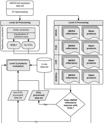
The standard MEGS processor (Case-2 water processing branch, Doerffer and Schiller, 1997; Doerffer, 2011) and three coastal processors that are provided as source-free plug-ins for the BEAM software, were used to derive the geophysical products (level 2 processing): the FUB proces-sor (Schroeder et al., 2007a, b), the Case-2 regional procesproces-sor C2R (Doerffer and Schiller, 2007) and the boreal lakes water processor BOREAL (Doerffer and Schiller, 2008). The gen-eral processing work flow can be seen in Fig. 2. The proces-sors assume environmental conditions of infinite deep water

Figure 2.Flow chart of the data processing work flow.

with vertical homogeneous distribution of water constituents, and no inelastic scattering or polarization effects are con-sidered. The derived geophysical products for each proces-sor used for the evaluation included algal pigments consid-ering chlorophylla as a proxy for biomass, here referred to as CHL, suspended particular matter and aCDOM (yellow substances). The yellow substances product (yellow_subs) of MEGS, C2R, BOREAL is the sum of yellow substance at 443 nm (YS) and the bleached particulate absorption (BPA) (Doerffer and Schiller, 1997; Doerffer, 2002; Doerffer and Schiller, 2007). In FUB this is referred to as yellow substance (Schroeder et al., 2007b). However, due to the relatively high aCDOM in the Baltic Sea in relation to non-pigmented par-ticles (Babin, 2000; Kowalczuk et al., 2006), in this study it is assumed that yellow substance mostly refers to the absorp-tion of CDOM, and that aCDOM≫BPA.

Table 2.Level 1b processing schemes applied.

Acronym Description

SC Smile correction

EQ Equalization of coherent noise

SCEQ_L1N Data set with both SCEQ corrections where ICOL has been applied SCEQ_X Data set with both SCEQ corrections where ICOL has not been applied

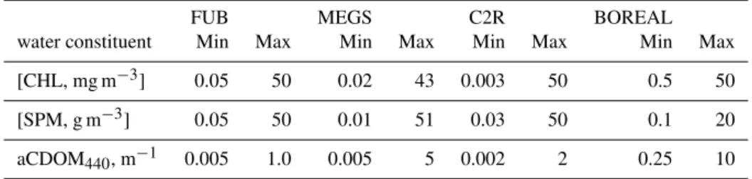
Table 3.Ranges of optical water constituent concentrations that define the training range of level 2 processors used here.

FUB MEGS C2R BOREAL

water constituent Min Max Min Max Min Max Min Max

[CHL, mg m−3] 0.05 50 0.02 43 0.003 50 0.5 50

[SPM, g m−3] 0.05 50 0.01 51 0.03 50 0.1 20 aCDOM₄₄₀, m−1 0.005 1.0 0.005 5 0.002 2 0.25 10

2.4 Macro pixel quality and exclusion criteria

Along the Swedish coast the typical current velocity in the Baltic Sea ranges from 2 to 5 cm s−1 (Maslowski and Walczowski, 2002). Considering 5 cm s−1 to be a fast-moving current in the study area, the water mass may move a maximum of 180 m in 1 hour, and in 2 hours the water mass may thus move about one MERIS pixel. A matrix of 3×3 pixels centred at the field sample location has been used to cover the natural variability of water displacement. There-fore, only those casts that were sampled during a matchup time window within the satellite overpass of 2 h or less (Ta-ble 1) have been selected for validation.

Each processor can raise flags at different stages of pro-cessing. These flags provide additional information regard-ing surface type (i.e. land, water, cloud); they also provide confidence information when the algorithm input or output is outside the expected range. Therefore, the macro pixels that represent water were filtered by flags, and pixels within the macro pixel were excluded if a flag was raised accord-ing to Table 4 (note that for geophysical products different terms are used by different authors and here the nomencla-ture is standardized for consistency throughout the paper, i.e. CHL for algal_2 and chl_conc; SPM for total_susp and tsm; aCDOM for yellow_subs and a_y_443). Only macro pixels with five or more non-flagged pixels were kept for further analysis and their pixel values were averaged (Kratzer and Vinterhav, 2010). The value of each macro pixel was as-sumed to represent the local conditions of the station cast for a given date. Due to the horizontal heterogeneity caused by the cyanobacterial blooms, a certain degree of variability within macro pixels is to be expected. Furthermore, coastal processes, fronts and natural gradients that may occur in the water body also add to this natural variability in the coastal zone. Nevertheless, after applying the exclusion criteria, the

macro pixels were considered to have minimum horizontal heterogeneity for coastal conditions and obviously do not represent oligotrophic conditions. Therefore, the homogene-ity test proposed by Bailey and Werdell (2006) to minimize the impact of geophysical variability within the macro pixels was modified to derive only those pixels after being filtered by the quality flags and minimum required pixels. The bias was calculated by using the standard deviation of the remain-ing “viable” pixels. This represents the minimum error that relates to the natural variability within the 3×3 pixel window. Each processor may result in a different set of viable macro pixels. In order to ensure that all water quality esti-mates from the different processors compare the same pix-els only those pixpix-els that are common within a viable macro pixel for each processor were used to derive the macro pixel averaged value for comparison. For the radiometry only com-mon macro pixels between all processors were used to assess the differences. For water products common macro pixels for each product among the pair of processors being compared are used for the analysis. This maximizes the number of vi-able macro pixels availvi-able for the differences estimates and ensures a fair comparison between the processors, i.e. the processors deal with the same pixels and observing condi-tions to derive the respective geophysical products.

For each processor the derived MERIS reflectanceρw(λ) from the ICOL-based processing scheme (SCEQ_L1N) and non-ICOL processing (SCEQ_X) were compared by calcu-lating the percentage differences:

δ[%] =ρw(λ)ICOL−ρw(λ)noICOL

ρw(λ)ICOL+ρw(λ)noICOL

Table 4.Quality flags used for pixel exclusion criteria within a 3×3 pixel matrix.

L2 processor Geophysical product Raised flags

MEGS algal_2, yellow_subs, total_susp land, suspect, pcd_1_13, pcd_17

radiometry land, suspect, pcd_1_13

FUB algal_2 LEVEL1b_masked, CHL_IN, CHL_OUT

yellow_subs LEVEL1b_masked, YEL_IN, YEL_OUT

total_susp LEVEL1b_masked, TSM_IN, TSM_OUT

radiometry LEVEL1b_masked, l1_flags>2, ATM_OUT

C2R chl_conc, a_ys_443, tsm case2_flags, agc_flags, l1_flags>2,

radiometry agc_flags, l1_flags>2

BOREAL chl_conc, a_ys_443, tsm case2_flags, agc_flags, l1_flags>2,

radiometry agc_flags, l1_flags>2

2.5 Comparison of MERIS-derived data products with in situ measurements

For each processor the derived MERIS reflectance ρw(λ) from the ICOL-based processing scheme (SCEQ_L1N) and non-ICOL processing (SCEQ_X) were compared against the in situ TACCS data. Note that in this study the radiometric standard products of MEGS were considered (Antoine and Morel, 2011) and not the intermediate products of the neural nets that refer to the Case-2 Branch. Common macro pix-els among the two processing schemes were selected and the sum of absolute differences against in situ data (SABS_D, Eq. 3) were calculated. These were then used to estimate the percentage of change between the two processing schemes (1ICOL, Eq. 4). Here, the SCEQ_X processing was used as a reference to evaluate the direction of change. A negative value of the1ICOLindicates a reduction of SABS_D for the SCEQ_L1N processing.:

SABS_D=

ncasts X

i=1 ρw(λ)

MERIS

i −ρw(λ)TACCSi

(3)

1ICOL=

(SABS_DSCEQ_L1N−SABS_DSCEQ_X) SABS_DSCEQ_X

×100 (4)

The validation was carried out over the data sets that had improved the MERIS reflectance for each processor. The ICOL-processed data sets (SCEQ_L1N) were the ba-sis of the water product (CHL, SPM and aCDOM) valida-tion, i.e. all level 2 products were smile corrected, equalized and a test on ICOL was performed. Based on the study of Kratzer and Vinterhav (2010) the ICOL-processed data were tested and worked as expected (i.e. reducing the land adja-cency effects for pixels within 15–20 km to coast), therefore their basis for further data processing and statistical evidence

was gathered to have substantially improved the MERIS re-flectance retrieval for each processor. The data sets derived from SCEQ_L1N were then used to assess the differences in ρw(λ)retrieval amongst processors compared to in situ data. Pair-wise comparison of the mean values of viable macro pixels to in situ data were then used for the analysis. Differ-ences were quantified statistically by using the mean normal-ized bias (MNB, Eq. 5) which is an estimate of systematic errors assuming that the in situ data are a “true” values; the root mean square of relative differences (RMSRD, Eq. 6) that indicates dispersion in the retrieval:

MNB=mean

"

yMERIS_i −x_iinsitu x_iinsitu

#

×100, (5)

RMSRD=SD "

y_iMERIS−x_iinsitu xinsitu_i

#

×100, (6)

wherei=1. . .is the number of averaged macro pixels, and “mean” and “SD” refer to the calculations of the mean (Eq. 7) and standard deviation value (Eq. 8), respectively:

mean=χ=1

n n X

i=1

χi, (7)

SD=

v u u t

1 n−1

n X

i=1

(χi−χ )2, (8)

Table 5.Range of concentrations of in situ water constituents.

In situ

Water constituent mean [median]±SD n Min Max

[CHL, mg m−3] 3.98[2.68] ±3.60 38 0.92 22.53

[SPM, g m−3] 1.46[1.34] ±0.69 38 0.30 3.25

aCDOM440, m−1 0.45[0.40] ±0.11 17 0.36 0.82

3 Results

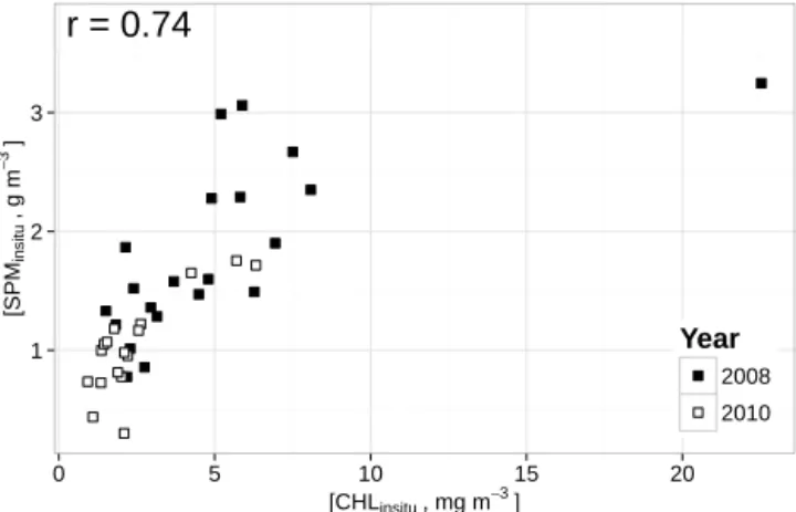
The observed ranges of in situ concentrations of Chl a, SPM and aCDOM for the two sea-truthing campaigns are presented in Table 5. The median chlorophyll concentra-tion measured in situ was about 2.7 mg m−3, the median SPM concentration was about 1.3 g m−3 and the median g440 (CDOM absorption at 440 nm) was 0.4 m−1. The sea-truthing data were found within the training ranges of the used level 2 processors (Tables 5 and 3) except for aCDOM during 2008. The in situ Chlaand SPM had a positive corre-lation,r=0.74 (data from 2008 and 2010, Fig. 3). Low cor-relation values were found for aCDOM vs. Chla(r=0.02) and aCDOM vs. SPM (r=0.18) when the cast ID H4_6a is excluded as this single value was identified as an outlier of normal conditions (data from 2010 only, as there were no aCDOM data for 2008).

The ranges of optical properties differed substantially for the two sea-truthing campaigns in 2008 and 2010. A higher range of concentrations for Chl a and SPM were observed in 2008. A smaller range of Chl a and SPM values were found for the sea-truthing data in 2010 (during full nitro-gen treatment), whilst data from 2008 (no nitronitro-gen treat-ment) generally had a greater range of values and were more variable. Station H5_3a in 2008 (Fig. 3) was found to be an outlier with the highest Chl a and SPM values. This was during a strong cyanobacterial bloom in which usually the relationship between satellite data and truthing data breaks down because of strong patchiness of the wa-ter body and strong horizontal hewa-terogeneity, making it dif-ficult to compare the satellite retrievals to truthing data. Wa-ter transparency as measured by Secchi depth showed less-transparent waters in 2008 with an average of 4.42±1.56 m compared to 6.45±1.65 m in 2010. In 2008, a Secchi depth minimum value of 1.9 m was observed at station H5, with Secchi depths increasing towards the outer Himmerfjärden stations. The Secchi depth was not found to be above 3 m in 2008 for the inner stations H5 and H4; Station H3 showed a Secchi depth range of 2.9–3.5 m and for H2 Secchi depth ranged between 3.4 and 4.1.

3.1 MERIS reflectance evaluation

For MEGS and FUB, the use of ICOL increased the number of viable macro pixels that previously had been flagged by

r = 0.74

1 2 3

0 5 10 15 20

[CHLinsitu, mg m− 3

]

[SPM

insitu

, g m

−

3]

Year 2008

2010

Figure 3.Correlation between [SPM] and [CHL]. The correlation coefficient,r, was calculated for both years.

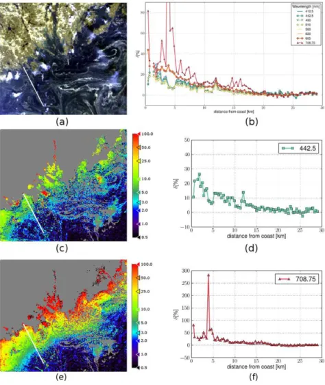
the macro pixel quality and exclusion criteria applied. Ra-diometric products derived after ICOL processing reduced the reflectance for previous overestimations and also reduced underestimations, especially in the blue-green region of the spectrum. The result is less flagging by each processor by correcting for atmospheric effects (in this case atmospheric scattering or stray light from land) prior to atmospheric cor-rection performed by each processor. An example of the spa-tial distribution of the percentage difference on MERIS re-flectance (image from 28 July 2008, during a cyanobacterial bloom) using FUB, when ICOL and no ICOL processing was applied (δ [%], Eq. 2) is shown for selected wavelengths, 443 nm (Fig. 4c) and 708 nm (Fig. 4e). The extracted pro-file ofδ[%] along a transect, from coast to open sea waters (representing the CI, CII, CIII stations), is given for all the available FUB bands and for the selected wavelengths (443 and 708 nm), see Fig. 4b, d, f, respectively.

The number of available macro pixels for the processor MEGS without using ICOL was 17, and after ICOL there were 24 macro pixels, i.e. an increase of 41 % of viable pix-els. The number of available macro pixels for FUB after ICOL processing were 19, an increase of 35 %. For the loca-tions H2 and H3, only FUB could retrieve the reflectance reli-ably. The number of available macro pixels for both C2R and BOREAL was 27 with no change on the available pixels af-ter ICOL processing. Based on these results, the ICOL-based data sets were used for the following comparison of level 2 products derived from all processors. Common macro pixels used to evaluate the retrieval ofρw(λ)resulted in 16 common macro pixels among the four processors after macro pixel quality control and exclusion criteria using the SCEQ_L1N data sets.

Figure 4.Example of spatial distribution and profile plots of the percentage difference in MERIS reflectance using FUB, when ICOL and no ICOL processing has been applied.(a)RGB composite;(b)reflectances in all channels show a logarithmic decline as expected;(cand d)percentage difference in the blue channel;(eandf)percentage difference in the NIR channel at 709 nm. The peak at about 4 km distance from land in the NIR is most likely caused by surface scum.

exponential decay of adjacency corrections when moving to-wards the open sea (Fig. 4b). The ICOL correction is no-table up to 20 km (Fig. 4b, c, d, e, f), with lowerδ towards the blue wavelengths. Higher δ values (>10 %) can be ob-served for the first 5 km in all bands. Beyond 15 km offshore δ are below 8 % for all selected bands, except for 708 nm. The red band at 708 nm, shows the highestδwith range val-ues 10–300 % within the first 10 km (Fig. 4b, f). After 10 km the differences found in this wavelength are similar to the other bands (Fig. 4b, d, f).

In general, FUB and MEGS estimates showed bias, thus an underestimation of ρw(λ) showed up in all bands com-pared to sea-truthing data (Table 6). The FUB processor underestimated ρw(λ) by between 22 % and 32 %, while MEGS underestimates by 7–16 % in the spectral bands above 443 nm. For MEGS ρw(λ) estimates the highest underesti-mations (35 %) were found at 413 nm. On the other hand,

an overestimation was found for C2R for the blue spectral bands, while the lowest bias occurs for the green spectral bands at 510 and 560 nm (1.1 and 8 %, respectively) for this processor. It may be pointed out that the highest uncertainty in the TACCS estimates occurs in the red channels (Zibordi et al., 2012), but the satellite retrieval amongst processors was most consistent in the red.

Table 6.Summary of error analysis forρ(λ)against sea-truthing data using common macro pixels (n=16). MERIS data set process-ing chainSCEQ_L1N-Smile Corrected and Equalized with ICOL.

Processor λ MNB [%] RMSRD[%] r

FUB 413 −23.38 35.91 0.11

443 −26.86 26.66 0.35 490 −22.18 18.47 0.66 510 −26.33 13.82 0.77 560 −29.28 11.76 0.84 620 −29.70 16.59 0.75 665 −32.58 16.19 0.77

MEGS 413 −35.23 65.87 0.33

443 −18.91 41.47 0.47 490 −12.67 21.52 0.77 510 −15.71 17.25 0.82 560 −12.84 13.39 0.91 620 −6.65 17.72 0.84 665 −10.04 19.47 0.78

C2R 413 28.10 81.60 0.52

443 20.38 61.70 0.56

490 17.64 43.92 0.69

510 −1.12 28.28 0.78 560 −8.01 17.99 0.87

620 4.55 20.46 0.81

665 −12.26 19.58 0.77

Figure 5.Correlation between MERIS and TACCSρw(λ)for each processor using common macro pixels. The solid black line repre-sents the 1:1 line. The correlation coefficient is given byr. The fig-ure columns represent selected wavelengths: blue (443 nm), green (560 nm) and red (665). The C2R and BOREAL had the same re-sults, so only the C2R is presented here.

Figure 6.Correlation for the pairwise [CHL] and [SPM] compari-son between FUB vs. MEGS(a, b)compared to sea-truthing mea-surements. Data correspond to common macro pixels. The error bars are the standard deviation of the macro pixel. The solid black line represents the 1:1 line.

3.2 CHL evaluation

In general, all processors overestimated the CHL concentra-tion. FUB was found to have the lowest bias and dispersion (Table 7). FUB showed an overestimation of chlorophyll of about 18–27 %, depending on the compared pairs after macro pixel exclusion criteria. MEGS showed an overestimation of 57–62 %. The dispersion of FUB were consistent among pairs with RMSRD values not higher than 55 %, while C2R dispersion varied among pairs and was above 104 %. MEGS dispersion was intermediate between 77 and 87 %. BOREAL presented the highest bias and dispersion in all pairs (Ta-ble 7). FUB showed less variability at lower CHL concen-trations (e.g.<4 mg m−3_{, Fig. 6a) than C2R and MEGS.} 3.3 SPM evaluation

The MEGS processor was the most accurate in retrieving SPM, while systematic overestimations were obtained with the MEGS, C2R and BOREAL processors. Only with the FUB processor were the SPM loads underestimated in all compared pairs (Table 8). When compared to FUB a MNB of only about 8 % was obtained by MEGS, whereas an underes-timation of 28 % was found for the FUB processor. The C2R retrievals were also satisfying when the processor was com-pared (pairwise with FUB and MEGS) to in situ measure-ments (5.5 and 25.21 %, respectively). Data scatter (noise) expressed by the RMSRDwas mainly found in the range of 40–50 % among all processors, with the exception for BO-REAL. The BOREAL estimates showed the highest noise with values above 60 %.

Table 7.Summary of error analysis for [CHL] compared to sea-truthing using common macro pixels by each pair of processors. MERIS data set processing chainSCEQ_L1N-Smile Corrected and Equalized with ICOL.

Pair Processor n MNB [%] RMSRD[%]

FUB_MEGS FUB 16 26.53 54.46

MEGS 62.23 86.93

C2R_FUB C2R 21 73.59 119.65

FUB 17.77 52.28

C2R_MEGS C2R 21 82.83 109.91

MEGS 56.76 77.38

BOREAL_MEGS BOREAL 11 241.39 169.70

MEGS 96.45 81.51

BOREAL_FUB BOREAL 11 266.79 211.02

FUB 45.79 53.48

BOREAL_C2R BOREAL 14 239.22 193.90

C2R 110.14 104.86

3.4 aCDOM evaluation

All processors underestimated aCDOM (Table 9). MEGS and C2R were not able to resolve the in situ aCDOM dis-tribution as all the retrieved macro pixels estimated similar aCDOM values (Fig. 7). FUB was able to resolve changes in aCDOM, albeit with a systematic underestimation when compared to in situ values. Figure 8 shows the regression equation obtained between FUB retrieved and in situ mea-sured aCDOM that can be used as local correction factor in order to improve the aCDOM retrieval. However, it must be noted that this regression will only be valid for the range of concentrations investigated here.

The results confirm the challenges to estimate aCDOM in the Baltic Sea accurately when a limited data set is applied to the present processors. In this study, 17 in situ aCDOM samples from 2010 were available for satellite validation. As mentioned before, the aCDOM field measurements for 2008 were not available. After applying the macro pixel quality control and exclusion criteria during the pairwise combina-tion, a reduced number of macro pixels were available to per-form the comparisons with in situ data. The pairwise combi-nation of C2R vs. FUB showed the maximum available pix-els, with only seven macro pixels left. The quality control of BOREAL when common macro pixels are used in the pair-wise comparison left only one or two viable pixels to make such comparisons, making it impossible to evaluate. 3.5 CHL and SPM evaluation by year

Using all available individual macro pixels for FUB (n=26, 16 and 10 observations in 2008 2010, respectively), the CHL retrievals (Table 10) showed lower bias for 2008 than 2010 (MNB = 16 and 24 %, respectively). The dispersion obtained

Table 8.Summary of error analysis for [SPM] compared to sea-truthing data using common macro pixels by each pair of pro-cessors. MERIS data set processing chainSCEQ_L1N-Smile Cor-rected and Equalized with ICOL.

Pair Processor n MNB [%] RMSRD[%]

FUB_MEGS FUB 16 −27.46 43.66

MEGS 7.85 39.87

C2R_FUB C2R 21 5.50 50.56

FUB −37.05 42.46

C2R_MEGS C2R 21 25.21 47.81

MEGS 16.16 42.42

BOREAL_MEGS BOREAL 11 76.95 61.82

MEGS 35.70 33.53

BOREAL_FUB BOREAL 11 47.52 78.52

FUB −25.90 42.64

BOREAL_C2R BOREAL 14 54.87 73.11

C2R 32.54 47.71

Table 9.Summary of error analysis for aCDOM compared to sea-truthing data using common macro pixels by each pair of pro-cessors. MERIS data set processing chainSCEQ_L1N-Smile Cor-rected and Equalized with ICOL.

Pair Processor n MNB [%] RMSRD[%]

FUB_MEGS FUB 5 −68.35 7.04

MEGS −89.89 2.56

C2R_FUB C2R 7 −88.71 2.68

FUB −68.64 5.16

C2R_MEGS C2R 6 −89.11 2.38

MEGS −90.08 2.34

with the FUB processor was higher for 2010 than 2008 (108 and 61 %, respectively). Biases of 57 % and 56 % were ob-tained with the MEGS processor for 2008 and 2010, respec-tively. Using MEGS, the total number of retrieved macro pix-els for CHL was 21 (15 observations in 2008 and 6 observa-tions in 2010). Data dispersion was above 69 % for both years (RMSRD70 % and 102 %, 2008 and 2010 respectively). Sus-pended particulate matter showed lower bias and data disper-sion in 2010 than in 2008 (MNB =−1 %, RMSRD=43 %) using MEGS (Table 10). FUB underestimated SPM in both years by 47 %. The C2R processor was the only processor retrieving the same number of macro pixels regardless of the water product (n=27). FUB and MEGS retrieved fewer in-dividual macro pixels for SPM than for CHL (macro pixel ratio SPM/CHL 19/26 FUB and 15/21 for MEGS).

Figure 7. Histogram showing the distribution of macro pixel CDOM absorption [m−1] for each level 2 processors.

Figure 8.Regression of aCDOM derived from FUB compared to sea-truthing data.

CHL vs. sea-truthing for 2008 and may add a clear bias to the results as this station was not retrieved by MEGS after the macro pixel quality and exclusion criteria were applied for the same year. Furthermore, the open-sea stations CI, CII and CIII, which are in a different sub-catchment and repre-sent a different water body than the stations within and close to the Himmerfjärden bay, were therefore also removed from the comparison.

Higher ranges of CHL values and variability was ob-served during 2008 than in 2010, for both processors (Table 11). MEGS had lower bias in 2008 (MNB=

23.1 %) and reduced dispersion (RMSRD=36.9) than FUB (MNB = 28.5; RMSRD=37.1). However, in 2010 the op-posite performance occurred for MEGS (MNB=55.8; RMSRD=102.0), FUB being more accurate (MNB = 24.1; RMSRD=108.2).

Suspended particulate matter bias and dispersion in FUB and MEGS remained without change after using the subset of individual macro pixels. The inner stations within Himmer-fjärden show a higher discrepancy to the sea-truthing data in 2008 for both processors.

Table 10.Summary of error analysis for [CHL] and [SPM] by year compared to sea-truthing data using individual best macro pixels. MERIS data set processing chainSCEQ_L1N-Smile Corrected and Equalized with ICOL.

Processor Water product Year n MNB [%] RMSRD[%]

FUB [CHL] 2008 16 15.5 60.9

2010 10 24.1 108.2 both 26 18.8 80.4

[SPM] 2008 9 −47.0 55.8

2010 10 −40.2 50.4 both 19 −43.4 51.6

MEGS [CHL] 2008 15 56.6 70.0

2010 6 55.8 102.0 both 21 56.4 77.6

[SPM] 2008 9 22.5 51.7

2010 6 −0.9 42.3 both 15 13.1 48.0

C2R [CHL] 2008 19 58.9 95.5

2010 8 88.9 134.3 both 27 67.7 106.6

[SPM] 2008 19 19.6 55.4

2010 8 3.8 46.6

both 27 14.9 52.6

Nevertheless, caution is advised in the interpretation of re-sults using individual macro pixels because they cannot be directly compared between FUB and MEGS; they represent their individual best, and they may not share the same ob-served macro pixels (as in the previous sections), thus they are likely to show discrepancies because the same pixels may not be compared. However, this comparison highlights the processor individual performance and its potential limi-tations within Himmerfjärden and adjacent areas.

4 Discussion

The results from the processors have shown less accurate ρw(λ)retrievals in the blue spectral region and better agree-ment in the green-red spectral region, similar to other opti-cally complex coastal water bodies (Park et al., 2004). Rela-tively lowρw(λ)in situ values in the blue bands 413 and 443 can be expected as the optical properties of the Baltic Sea are dominated by aCDOM (Schwarz et al., 2002; Darecki and Stramski, 2004; Reinart and Kutser, 2006) and SPM is low (Park et al., 2004).

Table 11. Summary of error analysis for [CHL] and [SPM] by year compared to a subset of sea-truthing data using individual best macro pixels. MERIS data set processing chainSCEQ_L1N-Smile Corrected and Equalized with ICOL.

Processor Water product Year n MNB [%] RMSRD[%]

FUB [CHL] 2008 9 −28.5 37.1

2010 10 24.1 108.2 both 19 −0.8 84.8

[SPM] 2008 9 −47.0 55.8

2010 10 −40.2 50.4 both 19 −43.4 51.6

MEGS [CHL] 2008 9 23.1 36.9

2010 6 55.8 102.0 both 15 36.2 69.0

[SPM] 2008 9 22.5 51.7

2010 6 −0.9 42.3 both 15 13.1 48.0

a further improvement of the standard radiometric products when ICOL is applied. However, Zibordi et al. (2013) rec-ommended that the resulting MERIS reflectances that result from the Case-2 water branch processing should be added to the MERIS standard data products. This would facilitate the assessment especially in relation with the creation of climate data records.

Surface accumulations of Cyanobacteria may increase the percentage difference of ICOL and no ICOL-based data sets. The observed higherδvalues at 708 nm (Fig. 4b, d) coincide with visible fronts caused by Cyanobacteria (Fig. 4a). These high peaks at 708 nm are also coincident with aδ decrease observed in the blue-green bands (Fig. 4b, d), that suggest strong chlorophyll absorption (Fig. 4d). This result may be used to the development of a cyanobacterial surface accumu-lation flags which requires further research.

Differences in CHL and SPM retrievals by MEGS and C2R were observed. However, the MEGS Case-2 branch and the C2R share not only the same architecture, but the water and atmospheric neural networks used in their bio-optical model are also the same (at least for processors ver-sions used here for MEGS 8.1 and C2R 1.5.3, C. Mazeran, personal communication, 2013). Therefore, these differences may arise in the implementation of pre-corrections of the top of atmosphere (TOA) signal (e.g. smile and gaseous correc-tions) and in the use of predefined physical constants (i.e. the solar flux at theoretical wavelengths) that may scale up in the level 2 water products.

At lower in situ chlorophyll concentrations (mainly<2.5 mg m−3, Fig. 6) relatively large data dis-persion dominates the retrievals. FUB is more stable and accurate especially in the open Baltic Sea, while MEGS and C2R showed greater variability. This higher variability is expressed in C2R and MEGS as an overestimation with higher noise in the retrieval which is in agreement with the

findings of Zibordi et al. (2013) for the Baltic Sea. Low performance of the neural network processors occurs for decreasing pigment concentrations in waters dominated by CDOM absorption, as aCDOM and SPM become the dominate optical signals (Doerffer and Schiller, 2007). At relatively high aCDOM, these differences may also be linked to the relatively small ranges of in situ SPM and Chla concentrations in comparison to the higher range of the processors (Table 5). As a consequence, in MEGS and C2R, low chlorophyll concentrations may be overestimated, while higher concentrations may not be overestimated. This may lead to a reduced difference between higher and lower pigment concentrations. An expression of this effect may be a reduced contrast of the image over the same range of values in comparison to FUB.

Furthermore, Heim et al. (2008) mentioned that by us-ing the C2R in optically complex waters the main attribution of the total absorption goes towards the pigment absorption, leading to an overestimation of CHL at low chlorophyll con-centrations and hence an underestimation of aCDOM. This is consistent with findings of Attila et al. (2013) and González Vilas et al. (2011). Attila et al. (2013) have also suggested that C2R retrievals in the Baltic Sea can be improved by modifying the mean conversion factors of the specific inher-ent optical properties, SIOPs (i.e. the chlorophyll conversion factor and exponent), used to derive the chlorophyll concen-tration from the absorption of phytoplankton pigments by us-ing appropriate regional factors.

The concentration of suspended particulate matter was more accurate with MEGS. Zibordi et al. (2013) reported a similar indication of accurate retrieval of SPM for MEGS across various European seas. In the presented study here, FUB showed lower accuracies for SPM retrievals than MEGS and C2R. These underestimations occurred mostly within Himmerfjärden, for the stations H3, H4 and H2 of the 18 July 2008 and 15 July 2008 data sets. During 2008, the inner stations of Himmerfjärden were highly influenced by the release of nitrogen from the Himmerfjärden sewage treatment plant. Higher SPM and aCDOM values observed in 2010 at the station H4 (cast ID: H4_6a, Table 1). This sug-gests that the location of H4 may optically be strongly influ-enced by the effluent outflow of the Himmerfjärden sewage treatment plant.

(Stramski et al., 2004; Roesler and Boss, 2008). As the par-ticle concentrations increase (including phytoplankton cells, organic particles, and detrital particulates) the backscattering and thus reflectance increases, but parallel to this, the ab-sorption may increase due to high aCDOM, hence reducing the reflectance. Different phytoplankton communities may also affect the size and shape of the backscattering signal. Cyanobacteria have highly reflective gas vacuoles for regu-lating their buoyancy. Furthermore, they form dense aggre-gations having a non-uniform distribution vertically and hor-izontally affecting both the absorption and scattering ratios (Kutser, 2004).

The individual macro pixel evaluation for FUB and MEGS showed some limitations in the performance of both pro-cessors. The truthing data showed that within Himmerfjär-den Secchi depth was reduced and highly variable in 2008. Higher dissolved and suspended matter may have been re-leased into the bay during lack of nitrogen treatment induc-ing the stimulation of primary production by increased re-lease of the nutrients from Himmerfjärden sewage plant. Wa-ter transparency was therefore decreased. CDOM absorption may also have been increased beyond the limit of the aC-DOM range for FUB as indicated by the high absorption measured by the AC9 and also by increasedKd(490)values which are highly correlated to aCDOM. Vaiˇci¯ut˙e et al. (2012) found Secchi depth strongly correlated to aCDOM and SPM, and being the most influential factors explaining the discrep-ancies between MERIS-derived products and in situ data for Lithuanian coastal waters. High values of organic SPM during summer indicate the occurrence of cyanobacterial blooms, which may also add to the decreased light trans-parency indicated by lower Secchi depths. In Baltic Sea wa-ters, it is usually aCDOM that is the dominant optical compo-nent influencing Secchi depth, but it is known to be less vari-able over space and time than SPM (Kratzer and Tett, 2009), SPM contributing more to the variability in Secchi depth.

FUB showed the highest discrepancies for the stations where Secchi values<3.5 m were measured for both CHL and SPM. Dispersion seems to dominate the retrieval of FUB CHL within Himmerfärden bay (Table 11). MEGS performed better in 2008 for CHL (i.e. at high chlorophyll ranges) and it seems to be able to retrieve higher CHL con-centrations with high attenuation background. Although the sample size is very small, these results are consistent with the findings of Vaiˇci¯ut˙e et al. (2012) for the offshore area and in the plume area of the Curonian lagoon where even more turbid waters and higher aCDOM can be found. The authors found that the MERIS standard processor provided the best fit when compared to sea-truthing data. However, FUB was shown to flag less data than the standard processor (only 10 % of data were removed by FUB flags, whereas the standard processor removed 60 % of the matchups). In this study, FUB also flagged less data than MEGS as can be seen from the number of observations in the subset data set for 2010 (FUBn=10, MEGSn=6, Table 11). FUB seems to

have better agreement with sea-truthing data at low CHL val-ues (e.g.<4 mg m−3_{) and with lower variability for open-sea} stations. FUB SPM retrievals were mostly underestimated (Table 11), which may be related primarily to atmospheric variability and clouds. The training data set in FUB may not be representative for the natural patterns of SPM occurring in the region of interest, as the data set used for training the neural nets was from the COASTLOOC project (Babin, 2000) representing more frequently waters with higher SPM. Furthermore, the inner stations remain underestimated for SPM and CHL using FUB, which may also suggest atmo-spheric correction failure (Cristina et al., 2009; Kratzer et al., 2008) not detected by the water flags in FUB, combined with adjacency effects that may limit the accuracy of SPM and CHL retrieval within Himmerfjärden. MEGS was able to re-trieve SPM at lower concentrations than FUB for 2010, but MEGS may also be strongly affected by failure of atmo-spheric and/or adjacency correction for the inner stations in the bay (Table 11).

Further, the study of Sørensen et al. (2007) showed uncer-tainty of 5–20 % for deriving CHL with the spectrophotomet-ric method in an international intercomparison between lab-oratories. Taking this into account, the overall accuracies ob-tained in this study using FUB and MEGS for retrieving CHL from natural phytoplankton in coastal waters can be consid-ered satisfying with regards to bias. In the pairwise retrieval, chlorophyll was retrieved best using FUB with an overesti-mation between 18 and 26.5 % (MNB) and with a MNB of

−29 % (2008) and 24 % (2010) in the individual FUB–sea-truthing comparison, which means that CHL can be derived within 30 % bias. The error of measuring SPM for the sea-truthing method used here is about 10 % in situ, and the pair-wise retrieval showed MNB errors of 8–16 % for MEGS and

−28 to −37 for FUB in this study. However, the previous study by Kratzer and Vinterhav (2010) showed better SPM retrieval for FUB using MERIS data from the 2nd reprocess-ing with MNB−4 % in the open sea, and−15 % inside Him-merfjärden. For MEGS MNB was−22 % in the open sea, and−12 % inside Himmerfjärden.

5 Conclusions

We have presented a processing chain for MERIS full-resolution products which is dedicated to CDOM-rich wa-ters. Including the ICOL adjacency correction in the chain improves the accuracy of the generated marine reflectances as well as the derived water products when compared to sea-truthing data. Therefore it is recommended to include ICOL in coastal Baltic Sea Waters.

which become evident when deriving the percentage dif-ference between ICOL and non-ICOL processed data sets (Fig. 4).

Overall, all investigated processors overestimate CHL val-ues. Suspended particulate matter is retrieved better by all processors than the other water constituents. In the inver-sion process aCDOM strongly competes with CHL absorp-tion causing aCDOM to be underestimated, and this may also affect CHL and SPM retrievals.

FUB is more accurate in the retrieval of CHL. In MEGS data dispersion dominates the retrievals at low chloro-phyll<2.5 mg m−3.

MEGS is more accurate for SPM retrieval. FUB showed the highest discrepancies in SPM concentrations for stations with high atmospheric variability and where high Secchi depth<3.5 m was measured.

The choice of whether to use FUB or MEGS for retrieval of SPM in a given area of the Baltic Sea must be assessed against local conditions and ranges of optical components.

For future algorithm development in waters affected by high CDOM absorption it is therefore recommended to de-couple the aCDOM retrieval from the retrieval of the CHL absorption at 443 nm (where high absorption of both aC-DOM and CHL coincide), and instead use other spectral fea-tures of phytoplankton pigments in the longer wavelengths for chlorophyll retrieval, e.g. the chlorophyll peak in the red at about 665 nm.

Appendix A

Table A1.Acronym list.

Abbreviation Description Unit/Version Category

CHL, Chla Phytoplankton pigments with chlorophyllaas proxy mg m−3 Water constituent

SPM Suspended particulate matter g m−3 Water constituent

CDOM, aCDOM Coloured dissolved organic matter and its absorption measured at 440 nm m−1 Water constituent YEL-BPA Yellow substances and bleached particle absorption m−1 Water constituent AMORGOS Accurate MERIS Ortho-Rectified Geo-location Operational Software Software BEAM Earth Observation Toolbox and Development Platform v.4.10.3 Software ODESA Optical data processor of the European Space Agency Software

TACCS Tethered attenuation coefficient chain-sensor Field radiometry instruments MERIS MEdium Resolution Imaging Spectrometer Satellites and Sensors

ENVISAT ENVIronment SATellite Satellites and Sensors

MEGS MERIS ground segment development platform v.8.1 Level-2 processors FUB Freie Universität Berlin Water processor v.1.2.10 Level-2 processors

C2R Case 2 Regional v.1.5.3 Level-2 processors

BOREAL Lakes Boreal processor v.1.5.3 Level-2 processors

ICOL Improved contrast between ocean and land v.2.9.1 Level 1B data processing

EQ Equalization of coherent noise Level 1B data processing

SC Smile correction Level 1B data processing

IOP Inherent optical properties Optics and radiometry

VIS Visible light of the electromagnetic spectrum [380–750 nm] nm Optics and radiometry

NIR Near-infrared nm Optics and radiometry

TOA Top of atmosphere Geolocation

MNB Mean normalized bias Statistics

The Supplement related to this article is available online at doi:10.5194/os-10-377-2014-supplement.

Acknowledgements. This research was funded by the Swedish

National Space Board (Dnr. 99/09) and the European Space Agency (ESA, contract no. 21524/08/I-OL). The authors would like to thank the staff at Askö Laboratory for support during field work. Great thanks are due to Gerald Moore for further developing the TACCS processor and advice on radiometric measurements and calibrations. Thanks are also due to the ODESA forum com-munity, especially to Constant Mazeran, for valuable discussions and clarifications regarding the MEGS processor and Thomas Schroeder for answering questions regarding the architecture of FUB. Acknowledgements go to Helena Höglander, Therese Harvey and Ragnar Elmgren from Stockholm University, Ecology, Envi-ronment and Plant Sciences, for valuable contributions regarding the Swedish National Monitoring Data and descriptions of the Himmerfjärden sewage treatment plant nitrogen experiments. Thanks also go to ESA and ACRI-ST for developing ODESA, available at http://earth.eo.esa.int/odesa.

Edited by: O. Zielinski

References

ACRI-ST: The AMORGOS MERIS CFI (Accurate MERIS Ortho-Rectified Geo-location Operational Software) Software User Manual & Interface Control Document, pO-ID-ACR-GS-0003, 2011.

ACRI-ST: ODESA software distribution, Quick start guide, oDESA-ACR-QSG, 2012.

Antoine, D. and Morel, A.: ATDB 2.7. Atmospheric Correction of the MERIS observations Over Ocean Case 1 waters, Tech. Rep. 5, Laboratoire D’Océanographie de Villefranche, 2011. Attila, J., Koponen, S., Kallio, K., Lindfors, A., Kaitala, S., and

Ylöstalo, P.: MERIS Case II water processor comparison on coastal sites of the northern Baltic Sea, Remote Sens. Environ., 128, 138–149, 2013.

Babin, M.: COAstal Surveillance Through Observation of Ocean Colour (COAST-LOOC), Final Report, Project ENV4-CT96-0310, 2000.

Bailey, S. W. and Werdell, P. J.: A multi-sensor approach for the on-orbit validation of ocean color satellite data products, Re-mote Sens. Environ., 102, 12–23, doi:10.1016/j.rse.2006.01.015, 2006.

Barker, K.: MERIS Optical Measurement Protocols. Part A: In situ water reflectance measurements, CO-SCI-ARG-TN-008, 2011. Borges, A. V.: Do we have enough pieces of the jigsaw to

in-tegrate CO2 fluxes in the coastal ocean?, Estuaries, 28, 3–27, doi:10.1007/BF02732750, 2005.

Bourg, L. and Members of the MERIS Quality Working Group: MERIS 3rd data reprocessing. Software and ADF updates, Re-port no. A879.NT.008.ACRI-ST, contract No. 21091/07/I-OL, 2011.

Bouvet, M. and Ramino, F.: Equalization of MERIS L1b prod-ucts from the 2nd reprocessing, Tech. Rep. ESA TN TEC-EEP/2009.521/MB, ESA, 2010.

Carder, K. L., Hawes, S. K., Baker, K. A., Smith, R. C., Stew-ard, R. G., and Mitchell, B. G.: Reflectance model for quan-tifying chlorophyll a in the presence of productivity degra-dation products, J. Geophys. Res.-Oceans, 96, 20599–20611, doi:10.1029/91JC02117, 1991.

Cristina, S. V., Goela, P., Icely, J. D., Newton, A., and Fragoso, B.: Assessment of the water-leaving reflectances of the oceanic and coastal waters using MERIS satellite products in Sagres off the southwest coast of Portugal, J. Coast. Res., available at: http: //hdl.handle.net/10400.1/1106, 1479–1483, 2009.

Darecki, M. and Stramski, D.: An evaluation of MODIS and SeaW-iFS bio-optical algorithms in the Baltic Sea, Remote Sens. Envi-ron., 89, 326–350, doi:10.1016/j.rse.2003.10.012, 2004. Doerffer, R.: Protocols for the validation of MERIS water products

– PO-TN-MEL-GS-0043, Tech. Rep. 1, GKSS Forschungszen-trum Geesthacht, available at: https://earth.esa.int/workshops/ mavt_2003/MAVT-2003_801_MERIS-protocols_issue1.3.5.pdf (last access: 19 March 2014), 2002.

Doerffer, R.: ATBD 2.255. Alternative Atmospheric Correction Procedure for Case 2 Water Remote Sensing using MERIS, Algorithm Theoretical Basis Document (ATBD) Version 1.0, Helmholtz-Zentrum Geesthacht, 21502 Geesthacht, 2011. Doerffer, R. and Schiller, H.: ATBD 2.12. Pigment index,

sedi-ment and gelbstoff retrieval from directional water leaving re-flectances using inverse modelling technique. Doc. No. PO-TN-MEL-GS-0005, Algorithm Theoretical Basis Document (ATBD) 4, GKSS Forschungszentrum Geesthacht, Institute of Hydrophysics, 21502 Geesthacht Germany, 1997.

Doerffer, R. and Schiller, H.: The MERIS Case 2 wa-ter algorithm, Int. J. Remote Sens., 28, 517–535, doi:10.1080/01431160600821127, 2007.

Doerffer, R. and Schiller, H.: MERIS Lake Water Algorithm for BEAM, Algorithm Theoretical Basis Document (ATBD) Version 1.0, GKSS GmbH, 21502 Geesthacht, 2008.

Doerffer, R., Sorensen, K., and Aiken, J.: MERIS potential for coastal zone applications, Int. J. Remote Sens., 20, 1809–1818, doi:10.1080/014311699212498, 1999.

Elmgren, R.: Understanding Human Impact on the Baltic Ecosys-tem: Changing Views in Recent Decades, AMBIO, 30, 222–231, doi:10.1579/0044-7447-30.4.222, 2001.

European Space Agency: MERIS Product Handbook, avail-able at: http://envisat.esa.int/handbooks/meris/ (last access: 3 June 2013), 2011.

Franzén, F., Kinell, G., Walve, J., Elmgren, R., and Söderqvist, T.: Participatory Social-Ecological Modeling in Eutrophication Management: the Case of Himmerfjärden, Sweden, Ecol. Soc., 16, 27, doi:10.5751/ES-04394-160427, 2011.

González Vilas, L., Spyrakos, E., and Torres Palenzuela, J. M.: Neural network estimation of chlorophyll a from MERIS full resolution data for the coastal waters of Galician rias (NW Spain), Remote Sens. Environ., 115, 524–535, doi:10.1016/j.rse.2010.09.021, 2011.

Heim, B., Overduin, P., Schirrmeister, L., and Doerffer, R.: OCOC -from Ocean Colour to Organic Carbon, Proc. of the 2nd MERIS/(A)ATSR User Workshop, Frascati, Italy 22–26 Septem-ber 2008 (ESA SP-666, NovemSeptem-ber 2008), 2008.

IOCCG: Report 10. Atmospheric correction for remotely-sensed ocean-colour products, IOCCG, International Ocean-Colour Co-ordinating Group, Canada, CA, 2010.

Jeffrey, S. W. and Humphrey, G. F.: New spectrophotometric equa-tions for determining chlorophylls a, b, c1 and c2 in higher plants, algae and natural phytoplankton, Biochemie und Physi-ologie der Pflanzen, 167, 191–194, 1975.

Kajiyama, T., D’Alimonte, D., and Zibordi, G.: Regional Algo-rithms for European Seas: A Case Study Based on MERIS Data, IEEE Geosci. Remote S., 10, 283–287, 2013.

Kirk, J. T. O.: Light and photosynthesis in aquatic environments, Cambridge University Press, 2nd Edn., 1994.

Koponen, S., Ruiz-Verdu, A., Heege, T., Heblinski, J., Sorensen, K., Kallio, K., Pyhälahti, T., Doerffer, R., Brockmann, C., and Peters, M.: Development of MERIS lake water algorithms. Vali-dation report, ESRIN Contract No. 20436/06/I-LG, 2008. Kowalczuk, P., Stedmon, C. A., and Markager, S.:

Model-ing absorption by CDOM in the Baltic Sea from sea-son, salinity and chlorophyll, Mar. Chem., 101, 1–11, doi:10.1016/j.marchem.2005.12.005, 2006.

Kratzer, S.: Bio-optical Studies of Coastal Waters, Ph.D. thesis, University of Wales, Bangor. School of Ocean Sciences, Menai Bridge, Anglesey, LL59 5EY, UK, 2000.

Kratzer, S. and Tett, P.: Using bio-optics to investigate the extent of coastal waters: A Swedish case study, Hydrobiologia, 629, 169– 186, doi:10.1007/s10750-009-9769-x, 2009.

Kratzer, S. and Vinterhav, C.: Improvement of MERIS level 2 prod-ucts in Baltic Sea coastal areas by applying the Improved Con-tracttrast between Ocean and Land processor (ICOL)-data anal-ysis and, Oceanologia, 32, 211–236, 2010.

Kratzer, S., Brockmann, C., and Moore, G.: Using MERIS full resolution data to monitor coastal waters – A case study from Himmerfjärden, a fjord-like bay in the north-western Baltic Sea, Remote Sens. Environ., 112, 2284–2300, doi:10.1016/j.rse.2007.10.006, 2008.

Kutser, T.: Quantitative detection of chlorophyll in cyanobacte-rial blooms by satellite remote sensing, Limnol. Oceanogr., 49, 2179–2189, 2004.

Kutser, T., Paavel, B., Metsamaa, L., and Vahtmäe, E.: Mapping coloured dissolved organic matter concentration in coastal wa-ters, Int. J. Remote Sens., 30, 5843–5849, 2009.

Laur, H.: ENVISAT and ERS missions, in ATMOS 2012, Advances in Atmospheric Science and Applications, 18– 22 June 2012, Bruges, Belgium, European Space Agency, available at: http://congrexprojects.com/docs/12m06_docs2/3_ laur--envisat-ers.pdf?sfvrsn=2 (last access: 1 June 2013), 2012. Leppèaranta, M. and Myrberg, K.: Physical Oceanography of the

Baltic Sea, Springer Praxis Books, Springer Berlin Heidelberg, doi:10.1007/978-3-540-79703-6, 2009.

Maslowski, W. and Walczowski, W.: Circulation of the Baltic Sea and its connection to the Pan-Arctic region – a large scale and high-resolution modeling approach, Boreal Environ. Res., 7, 319–325, 2002.

MERIS_ESL: MERIS smile effect characterisation and correction, Tech. rep., ESA, technical note, 2008.

Mobley, C. D.: Light and Water, Radiative Transfer in Natural Wa-ters, Vol. 592, Academic Press, 1994.

Moore, G., Icely, J., and Kratzer, S.: Field Inter-comparison and val-idation of in-water radiometer and sun photometers for MERIS validation, Proceedings of the ESA Living Planet Symposium, Special Publication SP-686, 2010.

Morel, A. and Prieur, L.: Analysis of variations in ocean color, Lim-nol. Oceanogr., 22, 709–722, doi:10.4319/lo.1977.22.4.0709, 1977.

Nelson, N. B. and Siegel, D. A.: The Global Distribution and Dy-namics of Chromophoric Dissolved Organic Matter, Annu. Rev. Mar. Sci., 5, 447–476, doi:10.1146/annurev-marine-120710-100751, 2013.

Ohde, T., Siegel, H., and Gerth, M.: Validation of MERIS Level-2 products in the Baltic Sea, the Namibian coastal area and the Atlantic Ocean, Int. J. Remote Sens., 28, 609–624, doi:10.1080/01431160600972961, 2007.

Park, Y., Van Mol, B., and Ruddick, K.: Validation of MERIS water products for Belgian coastal waters, in: Proceedings of MERIS and AATSR calibration and geographical validation validation workshop, 1, ESA, Frascati, 2004.

Parsons, T. R., Maita, Y., and Lalli, C. M.: A manual of chemi-cal and biologichemi-cal methods for seawater analysis, XIV, Pergamon Press, Oxford, UK, 1984.

Philipson, P., Kratzer, S., Krusper, A., and Strömbeck: Final report – Satellite products development for water quality monitoring in the great lakes and Himmerfjärden, 2009.

Prieur, L. and Sathyendranath, S.: An Optical Classification of Coastal and Oceanic Waters Based on the Specific Spectral Ab-sorption Curves of Phytoplankton Pigments, Dissolved Organic Matter, and Other Particulate Materials, Limnol. Oceanogr., 26, 671–689, 1981.

Reinart, A. and Kutser, T.: Comparison of different satellite sensors in detecting cyanobacterial bloom events in the Baltic Sea, Re-mote Sens. Environ., 102, 74–85, doi:10.1016/j.rse.2006.02.013, 2006.

Roesler, C. S. and Boss, E.: In Situ Measurement of the Inherent Optical Properties (IOPs) and Potential for Harmful Algal Bloom Detection and Coastal Ecosystem Observations, in: Real-time Coastal Observing Systems for Marine Ecosystem Dynamics and Harmful Algal Blooms. Theory, instrumentation and modelling, edited by: Babin, M., Roesler, C., and Cullen, J. J., UNESCO Publishing, Paris, 2008.

Santer, R. and Zagolski, F.: ICOL ATBD, Tech. Rep. version 0.1, Université du Littoral, Wimereux, France, 2007.

Santer, R. and Zagolski, F.: ICOL-Improve contrast between ocean & land, ATBD-The MERIS Level 1-C, Tech. Rep. version 1.1, Université du Littoral, Wimereux, France, 2009.

Schroeder, T., Behnert, I., Schaale, M., Fischer, J., and Do-erffer, R.: Atmospheric correction algorithm for MERIS above case-2 waters, Int. J. Remote Sens., 28, 1469–1486, doi:10.1080/01431160600962574, 2007a.

Schroeder, T., Schaale, M., and Fischer, J.: Retrieval of atmospheric and oceanic properties from MERIS measurements: A new Case-2 water processor for BEAM, Int. J. Remote Sens., Case-28, 56Case-27– 5632, doi:10.1080/01431160701601774, 2007b.

absorp-tion by coloured dissolved organic matter (CDOM), Oceanolo-gia, 44, 209–241, 2002.

Sørensen, K., Grung, M., and Röttgers, R.: An intercompar-ison of in vitro chlorophyll a determinations for MERIS level 2 data validation, Int. J. Remote Sens., 28, 537–554, doi:10.1080/01431160600815533, 2007.

Stramski, D., Boss, E., Bogucki, D., and Voss, K. J.: The role of seawater constituents in light backscattering in the ocean, Prog. Oceanogr., 61, 27–56, doi:10.1016/j.pocean.2004.07.001, 2004. Strickland, J. and Parsons, T.: A practical handbook of seawater

analysis, Fisheries Research Board of Canada Series, Fisheries Research Board of Canada, 1972.

Vaiˇci¯ut˙e, D., Bresciani, M., and Buˇcas, M.: Validation of MERIS bio-optical products with in situ data in the turbid Lithuanian Baltic Sea coastal waters, J. Appl. Remote Sens., 6, 063568.1– 063568.20, 2012.

Zhang, T.: Retrieval of oceanic constituents with artificial neural network based on radiative transfer simulation techniques, Ph.D. thesis, Freie Universität, Berlin, 2003.

Zibordi, G., Ruddick, K., Ansko, I., Moore, G., Kratzer, S., Icely, J., and Reinart, A.: In situ determination of the remote sens-ing reflectance: an inter-comparison, Ocean Sci., 8, 567–586, doi:10.5194/os-8-567-2012, 2012.