www.atmos-chem-phys.net/10/9657/2010/ doi:10.5194/acp-10-9657-2010
© Author(s) 2010. CC Attribution 3.0 License.
Chemistry
and Physics
The complex dynamics of the seasonal component of USA’s surface
temperature
A. Vecchio1,2, V. Capparelli2, and V. Carbone2,3
1Consorzio Nazionale Interuniversitario per le Scienze Fisiche della Materia (CNISM), unit`a di ricerca di Cosenza, Ponte P. Bucci cubo 31C, 87036 Rende (CS), Italy
2Dipartimento di Fisica, Universit`a della Calabria, Italy 3Liquid Crystal Laboratory, IPCF/CNR, Italy
Received: 8 April 2010 – Published in Atmos. Chem. Phys. Discuss.: 23 June 2010
Revised: 21 September 2010 – Accepted: 26 September 2010 – Published: 11 October 2010
Abstract. The dynamics of the climate system has been investigated by analyzing the complex seasonal oscillation of monthly averaged temperatures recorded at 1167 stations covering the whole USA. We found the presence of an orbit-climate relationship on time scales remarkably shorter than the Milankovitch period related to the nutational forcing. The relationship manifests itself through occasional destabiliza-tion of the phase of the seasonal component due to the local changing of balance between direct insolation and the net en-ergy received by the Earth. Quite surprisingly, we found that the local intermittent dynamics is modulated by a periodic component of about 18.6 yr due to the nutation of the Earth, which represents the main modulation of the Earth’s preces-sion. The global effect in the last century results in a cumu-lative phase-shift of about 1.74 days towards earlier seasons, in agreement with the phase shift expected from the Earth’s precession. The climate dynamics of the seasonal cycle can be described through a nonlinear circle-map, indicating that the destabilization process can be associated to intermittent transitions from quasi-periodicity to chaos.
1 Introduction
The annual rotation of the Earth around the Sun provides a quasi-periodic solar forcing that continuously synchronizes the terrestrial climate. The resulting seasons observed on Earth represent the complex nonlinear response of atmo-sphere, land and oceans to this forcing and are one of the most important source of variability for the climate system.
Correspondence to:A. Vecchio ([email protected])
In fact, even if climate changes are usually referred to trends in the average temperature records (Alley et al., 2003; Karl and Trenberth, 2003), many studies have shown that the anal-ysis on the seasonal cycle of the Earth temperature could improve our knowledge about climate changes (Thomson, 1995, 1997; Huybers and Curry, 2006; Pezzulli et al., 2005; Stine et al., 2009). Unlike the external solar forcing, which is almost constant from year to year, there is no guarantee that climatic seasons have to be the same each year. Actually seasonal variations cause more than 90% of the variance of a temperature record and represent one of the basic exam-ples of the complex atmospheric response to external forcing (Thomson, 1995, 1997; Mann and Park, 1996; Wallace and Osborn, 2002; Jones et al., 2003; Stine et al., 2009).
Previous studies about the phase of the global seasonal-ity have underlined the presence of a phase shift. Thompson showed that, after 1940, the phase behavior started to change at an unprecedented rate with respect to the past 300 years (Thomson, 1995). Other authors indicated a global phase-shift towards earlier seasons (Mann and Park, 1996; Wal-lace and Osborn, 2002; Jones et al., 2003). A recent esti-mate (Stine et al., 2009) yields a global phase shift of the annual cycle of surface temperatures, over extratropical land between 1954 and 2007, of about1≃1.7 days. Even in this case the result seems to be highly anomalous with respect to the phase-shift of earlier periods.
The phase shift phenomenon has been attributed either to an increased temperature sensitivity to the anomalistic year forcing relative to the tropical year forcing due to Earth’s pre-cession (Thomson, 1995), or changes in albedo, soil moisture and short-wave forcing, also involved in changing modes of atmospheric circulation (Stine et al., 2009). The anomalous phase shift recorded after 1940 has been attributed to the in-creasing presence of CO2 in atmosphere (Thomson, 1995; Stine et al., 2009). The phase shift is not predicted by the current Intergovernmental Panel on Climate Change models (Stine et al., 2009), thus representing a yet rather obscure physical effect of the climate system. The role and exact ex-tent of natural and anthropogenic forcing for the climate evo-lution has been under much debate (Thomson, 1997; Keel-ing et al., 1996; Hasselmann, 1997; Rind, 2002; Alley et al., 2003; Karl and Trenberth, 2003; Scafetta and West, 2008), and any attempt to point out hidden aspects of climate dy-namics is of considerable interest.
2 Data analysis
In the present paper we focused on the phase of the seasonal oscillation by using an ensemble of temperature time se-riesT (t )from the United State Historical Climatology Net-work1. The data set covers 110 yr from 1898 up to 2008 and is recorded byN=1167 different stations distributed on the whole USA. The seasonal component has been identi-fied through the Empirical Mode Decomposition (EMD), a technique developed to process non-stationary data (Huang et al., 1998) and successfully applied in many different fields (Cummings et al., 2004; McDonald et al., 2007; Terradas et al., 2004; Vecchio et al., 2010). EMD decomposes the variance of each temperature record into a finite number of intrinsic mode functions (IMFs) and a residue, describing the mean trend, by using an adaptive basis derived from each data set (Huang et al., 1998), namely:
T (t )=
m X
j=0
θj(t )+rm(t ). (1)
1The HCN data set is available at http://cdiac.ornl.gov/epubs/
ndp/ushcn/ushcn.html
For a given time series, each IMF θj(t )has its very own
timescale and represents an oscillation with both amplitude and frequency modulations. This kind of decomposition is local, complete and in fact orthogonal (Huang et al., 1998; Cummings et al., 2004). The intrinsic mode functions yield instantaneous phases8j(t )and, after a time derivative, the
instantaneous frequenciesωj(t ). For all records, the highest
frequency IMF (j=0) represents the inter-seasonal stochastic component of the signal. High-order modes describe modu-lations of increasingly long periods, while the residuerm(t ) represents the monotonically increasing local trend of tem-perature, commonly attributed to large scale warming since the urbanization contribution is smaller (see Peterson, 2003; Parker, 2006; Jones et al., 2008). The seasonal oscillation is described by the modej=1 with a typical timescale of about
1τ1≃1 year. The statistical significance of information con-tent for each IMF with respect to a white noise has been checked by applying the test developed by Wu and Huang (2004).
The 66% of the stations show an anomalous seasonal os-cillation characterized by intermittent local decreases of the amplitude of thej=1 mode. For these stations the seasonal oscillation is spread over two EMD modes, namely the regu-lar season is rediscovered whenθ1(t )andθ2(t )are summed up. The remaining 34% of the stations shows a regular sea-sonal oscillation just isolated in thej=1 mode. An exam-ple from Evanston WY and Smithfield NC stations, char-acterized by regular and anomalous seasonal oscillation, re-spectively, is shown in Fig. 1 where the temperature records (panel a, b), the dynamics ofθ1(t )(panels c, d), the instan-taneous81(panels e, f) and unwrapped (panels g, h) phase, and the instantaneous frequency (panel i, j) are reported in a time interval of 30 yr. Each anomaly is associated with a strong variation of the instantaneous frequency and with an increasing phase-shift of the seasons, originating a destabi-lization of the phase81of seasonal oscillation. This phase shift is marked by steps in the unwrapped phase plot (panel h). All these features are not observed for the “regular” sta-tion (left column of Fig. 1). We have to remark that the am-plitudes of the modesθ1are all above the 99% confidence level with respect to a white noise (Wu and Huang, 2004).
In Fig. 2 the time evolution of the EMD modesj=1 and
Fig. 1.Examples of EMD results from Evanston WY record (right column), characterized by regular seasonal oscillations, and from Smithfield NC (left column), showing season anomalies in a 30 yr time interval. (a, b)refer to the rough data sets. The anomaly is underlined, in the right column, by the time evolution of: the IMF modeθ1(t )(d), the phase81(t )(f), the unwrapped phase(h)and the instantaneous frequency(j). These quantities have been calcu-lated by using the first EMD modej=1.
used, thus reducing the chance of mode mixing. By using the EEMD Wu et al. (2008) showed that the seasonal com-ponent of the analyzed temperature record is also spread over two modes. Our analysis indicates a correspondence between phase anomalies and spreading of seasonal oscillations over two modes. Hence it seems very interesting to investigate the role of the phase intermittency in the temperature records and to relate it to the physics of the system. To this purpose the EEMD approach does not seem suitable, since it repre-sents an ad hoc mechanism to cancel the intermittency from IMFs. On the contrary, if the goal of the research is to study the intermittency phenomenon in the analyzed signals, then we need to analyze the IMFs as they are obtained by EMD. In this way an IMF, although affected by mode mixing, can be useful to identify when intermittency is present. More-over, because of their orthogonality, IMFs, differently from EEMD modes, can be given some more direct physical inter-pretation. The EMD is a technique developed to be highly sensitive to the local frequency (or phase, beingω=dφ/dt) fluctuations. For records showing irregular seasonal oscil-lations the frequency is slightly different form the expected
Fig. 2.Time evolution of the EMD modesj=1 andj=2(a, b)and their sum(c)for the temperature record in panel (b) of Fig. 1.
one during an anomaly. In these cases, the detection of two IMFs, necessary to describe the full contribution of the sea-son, results from the properties of the EMD decomposition for which each mode is associated to a well defined time scale. If a given time scale is present only during a small portion of the signal, namely 1t∗, the IMF describing this oscillation will be significantly different from zero only dur-ing1t∗. The modej=2 simply provides the value of the ”anomalous” frequency and the time intervals in which it oc-curs. The meaningful quantity is the sumθ1+θ2describing the full contribution of the seasonal cycle to the temperature record. In this application, the usefulness of EMD resides in its ability to highlight the periods in which the frequency of the season is anomalous. We have to remark that the EMD represents a powerful tool to deseasonalize the temperature record (see e.g. Vecchio and Carbone, 2010) by subtracting the reconstructed seasonality θ1+θ2 from the raw record. This kind of approach is more efficient than the classical deseasonalization procedured involving time averages, since the temperature records are far to be stationary.
Table 1. Main periodP of the anomalies occurrence calculated through a sinusoidal fit (first column) and from the dominant peak in the Fourier periodogram (second column).
sin fit Fourier
Method A 18.8±0.4 20±5 Method B 18.7±0.2 18.5±3.5
anomaly occurrence as a pointlike process, that is, each of them is supposed to occur at its starting timeti, we calculate
the waiting time distribution (WTD), namely the probability density of the time intervals between two consecutive events
P (1t ). Quite interestingly the detected phase-shift events are strongly correlated in time.
Two independent procedures have been developed to rec-ognize the time of occurrence of a season anomaly:
1. since an anomaly corresponds to a strong local varia-tion of the instantaneous frequency of the seasonal IMF, it can be identified with the formation of a spike in the local frequency (see Fig. 1 panel j). Since in princi-ple positive and negative excursions in frequency can occur, the time of occurrence of each season anomaly corresponds to the local maximum in the range where the absolute value of instantaneous frequency is greater than two standard deviations of its average
2. anomaly occurrence is detected from the j=2 IMF characterized by a temporal behavior like those shown in Fig. 2 panel b. For this mode, the amplitude increases in correspondence of the season anomalies. The points of each interval where the absolute value of the am-plitude exceeds two standard deviations of the chosen IMF are identified. For each interval the distance be-tween extreme points, satisfying the previous threshold, defines the duration of the anomaly and identifies it. The WTD calculated with the two different methods to identify anomalies, is shown in Fig. 3. An exponential shape of WTD corresponds to Poisson processes. In our case roughly equispaced peaks, superimposed to the exponential decay, can be recognized, thus indicating that the WTD is not associated to a stochastic process but there is a dominant periodicity. This is clear by looking at the binned occurrence of seasonal anomalies as a function of time (Fig. 4): phase-shift events show an oscillating behavior. The main period
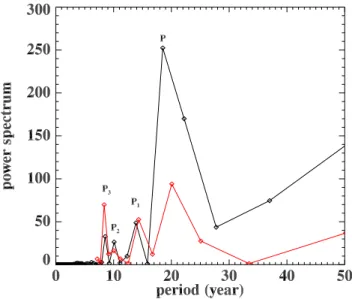
P of the anomaly occurrence has been calculated through a sinusoidal fit over the red and black curve of Fig. 4, and by identifying the dominant peak in the Fourier periodogram (Fig. 5). The results are shown in Table 1. The uncertainties have been calculated from the fitting procedure and from the Fourier period resolution at the found peak.
The value of the periodP is remarkably close to the 18.6-year period of the Earth’s nutation, which represents the
Fig. 3. Waiting time distribution for the anomalies of seasonality for all the 1167 stations. Red and black curves refer to the differ-ent methods 1. and 2., described in the text, used to iddiffer-entify the anomalies.
Fig. 4. Anomaly occurrence detected in our dataset. Red and black curves refer to the methods 1. and 2., described in the text, used to identify the anomalies. The period of modulation, cal-culated for both curves, is reported in Table 1. The blue curve refers to the cycle of the changing inclination of the Moon’s or-bit, with respect to the equatorial plane due to nutation, modeled byψ=23◦27′+5◦09′sin(Nt+π ), whereN=2π/18.6134 yr (cf.
Yndestad, 2006).
Fig. 5.Fourier power spectra for the anomaly occurrence detected in our dataset. Red and black curves refer to the methods 1. and 2.
between occurrence of seasonal anomalies (black curve in Fig. 4) and the inclination of the Moon’s orbit (blue curve) assumes the value 0.57.
Since the phase-shift anomalies cannot be considered as purely stochastic events, we are going to discuss the origin of the above periodicity. We think this is a strong evidence of nutational forcing on temperature records probably due to an influence of the anomalistic year variability on seasonal timing variability (see Thomson, 1995). The amplitude and phase variability of climate, which we call “season”, is de-termined by the competing action of the direct insolation, having its maximum at the perihelion, and the net radiation received by the Earth, having its maximum at the summer solstice. In the Northern Hemisphere, summer solstice and perihelion are about 180◦out of phase. Consequently, slight perturbation on either component can destabilize the system by changing the resultant proportionality. We can conjec-ture that the motion of the Earth’s axis due to the nutation, by affecting the insolation, can continuously perturb the cli-mate system. Due to strong nonlinearities in the atmospheric system, the climate response to the annual cycle of the so-lar forcing can be surprisingly abrupt, for example as it hap-pens in the case of the rapid onset of the Asian monsoon (Pezzulli et al., 2005). This coupling can generate impulsive destabilization of the phase which results in a global phase shift modulated by the nutation component. Being the tem-perature records strongly dependent on the local conditions, the nutation signal is detected only when a statistical analy-sis, over a significant number of stations, is performed. The above orbit-climate relation is amplified by the EMD, which is a technique extremely sensitive to the signal’s phase shifts. Three peaks, at low energy with respect to P, can be identified from the Fourier spectra of Fig. 5. They corre-spond to the periodsP1=13.9±0.6 yr,P2=10.1±0.8 yr,
P3=8.5±2.1 yr. Similar periodicities have been found in previous works. In detail,P1is consistent with the∼15 yr periodicity in coastal surface air temperature in the Gulf of Alaska (GOA) (Wilson et al., 2007) attributed to large-scale coherent Pacific climate variability. P2 could be related to the∼11 yr periodicity in ice core sequences (Royer, 1993) attributed to solar cycle effects. P3 might be attributed to changing tidal current speeds due to interannual variability of the lunar orbit, in particular to the 8.85 yr period of ro-tation of the lunar perigee around the Earth (McKinnell and Crawford, 2007). It must be remarked that a periodicity of about 7.8 yr has been also found in drought data (Cook et al., 1997).
3 A simple model that reproduces complex seasonality
To investigate the system response to the perturbation due to the nutation, the dynamics of the seasonal cycle has been described by the Phase Transition Curve (PTC), that is a ba-sic tool to investigate recurrent dynamics as the time evo-lution of an oscillating system (e.g. Arnold, 1965; Glass and Mackey, 1979; Croisier et al., 2009; Glass, 2001, and references therein). The PTC is a map describing the dy-namics of an angular variable αn, such that αn+1=f (αn)
wheref is a given function. In our case the variableαnis
identified with81(tn), namely the phase at a discrete time
tn (n=0,1,...). A regular season is described by a linear
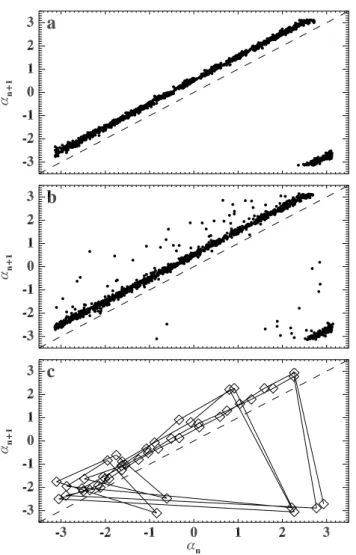
mapαn+1=(αn+ω0)mod(2π ), whereω0is the intrinsic fre-quency of the cycle. In Fig. 6 empirical PTCs are reported for the two stations of Fig. 1 (Evanston WY in panel a and Smithfield NC in panel b). In both cases, the dynamics of the PTC locally deviate from the linear behavior. For both maps the points are spread around the straight line, corre-sponding to the linear PTC, because of weak stochastic fluc-tuations due to random vagaries of the weather at monthly scales. Moreover, large excursions away from the linear dy-namics are observed in panel b) in correspondence of the anomalies. The graphic iteration of this PTC map around a detected anomaly, from 1972 to 1975, is shown in panel c). Nonlinearities of the climate system, that is the occurrence of fluctuations which occasionally destabilize the system, cause significant deviations from the linear dynamics.
The observed PTC, including the effect of anomalies, can be reproduced by a so-calledcircle map(Ott, 2002), that de-scribes the dynamics of a system characterized by two com-peting forcing with different frequencies. According to the general theory of dynamical systems (Ott, 2002), the cir-cle map, in presence of two forcing oscillations, can be ex-pressed in a linear form
φn+1=(φn+w)mod(2π ) (2)
Fig. 6.Phase Transition Curveαn+1=f (αn)calculated using the
data from Evanston WY(a)and from Smithfield NC(b)stations. An example of iteration of the panel (b) map around a given sea-sonal anomaly is reported in panel(c).
irrational the dynamics of the map is quasi-periodic, namely the orbit obtained from the iteration densely fills the circle as time goes to infinity (Ott, 2002). A nonlinear coupling between the external periodic forces is described by adding a functionf (φn)to the right hand side of Eq. (2). The most
fa-mous example is the sine-circle map investigated by Arnolds
φn+1=(φn+w+ksinφn)mod(2π ) (3)
wherekis a constant (Arnold, 1965; Ott, 2002). The pres-ence of the nonlinear term destroyes the quasi-periodicity in favor of the frequency locking because of the coupling thus generating an interesting transition to a chaotic state. Roughly speaking, the set of periodic points, which is of zero measure fork=0, increases ask6=0. For a fixed value ofk, the rotation number
r= 1 2πNlim→∞
N X
n=1
(w+ksinφn) (4)
as a function ofw is an intricate sequence of periodic and quasi-periodic regions (Ott, 2002). Since in our case w
changes because of the precession and nutation, the system moves into the net of periodic and quasi-periodic states and is continuously destabilized.
The empirical PTC (panel b in Fig. 6) indicates that during the seasonal anomalies the regular dynamics of the seasonal oscillation is destabilized. This can be described by conjec-turing that the frequency locking phenomenon depends on the nonlinear coupling with the atmosphere. In order to re-produce our result we modify the sine-circle map by adding a periodic perturbation of the winding number and a variable coupling parameterk,
φn+1= [φn+w+Rn+kn(Rn)sinφn]mod(2π ) (5)
where the periodic term related to the nutation is
Rn=R0cos(Ntn)and the parameterk(Rn)is not kept
con-stant and represents the response to this perturbation. In par-ticular, we conjecture that the response of climate to the orbit perturbation is a threshold phenomenon, so that the behavior ofkcan be described by the following map
kn+1=
kn if Rn≤Rth
znkn(1−kn)if Rn> Rth (6) whereRth is a threshold value. When the inclination of the Earth’s axis is greater than a critical value, the frequency locking of the seasonal cycle occurs abruptly. This can be re-produced for example by a simple on-off intermittent process (Platt et al., 1993). In this framework the parameterznis
suit-ably chosen to assume two values, sayzn=1/2 orzn=4 with
probabilitypand(1−p), respectively. When 1/3≤p≤0.47 the sequence ofknbehaves as a typical on-off intermittency
(Loreto et al., 1996). Results of the model Eqs. (5) and (6), reported in Fig. 7, reproduce the observed behavior.
4 Conclusions
Fig. 7.Results of the modified sine-circle map Eqs. (5) and (6) ob-tained with the following set of parameters (see text):R0=3×10⁻⁴, Rth=2.6×10⁻⁴, andp=0.43. In the upper panel we report the be-havior ofφnaround a given anomaly, while in the lower panel we
report the Phase Transition Curveφn+1=f (φn). Dashed line
cor-responds toφn+1=φn.
are remarkably close to the Earth’s nutation. The occurrence of local phase shifts causes significant deviations of the tem from the linear dynamics since the response of the sys-tem to this kind of perturbations is highly nonlinear. Our findings represent an indication that the phase of the sea-son is influenced by the Earth’s nutation. The global phase shift, underlined by different authors in the past (Thomson, 1995; Mann and Park, 1996; Wallace and Osborn, 2002; Jones et al., 2003; Stine et al., 2009), could be related to the global effect of the local dynamics of impulsive phase-shift events. EMD results indicate that each anomaly of the seasonal cycle of temperature corresponds to a local phase shift well identified by steps in the unwrapped phase plots. By making use of simple statistical arguments we investi-gate if the combined effect of the anomalies could result in a global phase shift of the temperatures as detected by some authors (Thomson, 1995; Mann and Park, 1996; Wallace and Osborn, 2002; Jones et al., 2003; Stine et al., 2009). This can be quantified by looking at the probability distributionP ()
of=w/ω0(Fig. 8), wherew=limn→∞[(φn−φ0)/2π n] is the theoretical winding number.represents the phase shift, with respect to the initial phase, detected for each station
Fig. 8. Probability of occurrence of the global phase-shift nor-malized to the yearly seasonal frequency, calculated for all 110 yr of our dataset.
from 1898 to 2008 and normalized to the intrinsic frequency
w0=25/12 months−1. values different from 1 indicate a phase shift toward earlier, if>1, or later, if<1, seasons. Thedistribution is asymmetrical towards values greater than one, thus indicating an average shift towards earlier sea-sons. The maximum is found around the value≃1.03 cor-responding to a phase shift of about1φ=|(1−)/ω0|≃1.74 days with a standard deviation of about 0.08 days. This result is in close agreement with the global shift estimated by Stine et al. (2009). Thus the combined effect of the single phase shift on each station gives rise to a weak global phase shift of the seasonal cycle of surface temperatures of 1.74 days towards earlier seasons over 110 yr in agreement with past results.
ocean-atmosphere model and without the need for any exter-nal forcing (Yasuda et al., 2006).
It must be remarked that our model represents just a simple example to explain the observed behavior of the USA’s tem-perature records, in terms of the variation of the insolation due to the nutation of the Earth. Previous papers, analyzing different climatic datasets, do not clearly indicate whether the bi-decadal periodicity is related to the variation of the in-solation due to the nutation of the Earth and/or lunar tidal forcing. This interesting topic will be the object of future investigations.
Acknowledgements. We acknowledge two anonymous referees for useful comments. We acknowledge M. Onofri, L. Sorriso-Valvo and A. Papa for useful discussions.
Edited by: A. Baumgaertner
References
Alley, R. B., Marotzke, J., Nordhaus, W. D., Overpeck, J. T., Peteet, D. M., Pielke, R. A., Pierrehumbert, R. T., Rhines, P. B., Stocker, T. F., Talley, L. D., and Wallace, J. M.: Abrupt Climate Change, Science, 299, 2005–2010, doi:10.1126/science.1081056, 2003. Arnold, V. I.: Small denominators. I. mappings of the
circumfer-ence onto itself., AMS Trans. Series 2(46), 213–284, 1965. Cook, E., Rosanne, D., Cole, J., Stable, D., and Villalba, R.:
Tree-ring records of past ENSO variability and forcing, in El Ni˜no and the Southern Oscillation: Multiscale Variability and Global and Regional Impacts, Cambridge Univ. Press, 2000.
Cook, E. R., Meko, D. M., and Stockton, C. W.: A New Assessment of Possible Solar and Lunar Forcing of the Bidecadal Drought Rhythm in the Western United States., J. Climate, 10, 1343– 1356, doi:10.1175/1520-0442(1997)010, 1997.
Croisier, H., Guevara, M. R., and Dauby, P. C.: Bifurcation analysis of a periodically forced relaxation oscillator: Differential model versus phase-resetting map, Phys. Rev. E, 79, 016209, doi:10. 1103/PhysRevE.79.016209, 2009.
Cummings, D. A. T., Irizarry, R. A., Huang, N. E., Endy, T. P., Nisalak, A., Ungchusak, K., and Burke, D. S.: Travelling waves in the occurrence of dengue haemorrhagic fever in Thailand, Na-ture, 427, 344–347, doi:10.1038/nature02225, 2004.
Currie, R. G.: Evidence for 18.6-year lunar nodal drought in West-ern North America during the past millennium, J. Geophys. Res. Ocean., 89, 1295–1308, doi:10.1029/JD089iD01p01295, 1984. Glass, L.: Synchronization and rhythmic processes in physiology,
Nature, 410, 277–284, doi:10.1038/35065745, 2001.
Glass, L. and Mackey, M. C.: A simple model for phase locking of biological oscillators, J. Math. Biol., 7, 339–352, doi:10.1007/ BF00275153, 1979.
Hasselmann, K.: Climate Change: Are We Seeing Global Warm-ing?, Science, 276, 914–915, doi:10.1126/science.276.5314.914, 1997.
Huang, N. E., Shen, Z., Long, S. R., Wu, M. C., Shih, H. H., Zheng, Q., Yen, N., Tung, C. C., and Liu, H. H.: The empirical mode decomposition and the Hilbert spectrum for nonlinear and non-stationary time series analysis, Royal Soc. Ldn. Proc. Ser. A, 454, 903–995, 1998.
Huybers, P. and Curry, W.: Links between annual, Milankovitch and continuum temperature variability, Nature, 441, 329–332, doi:10.1038/nature04745, 2006.
Imbrie, J. and Imbrie, J. Z.: Modeling the climatic response to orbital variations, Science, 207, 943–953, doi:10.1126/science. 207.4434.943, 1980.
Jiang, N., Neelin, J. D., and Ghil, M.: Quasi-quadrennial and quasi-biennial variability in the equatorial Pacific, Clim. Dynam., 12, 101–112, doi:10.1007/s003820050097, 1995.
Jin, F., Neelin, J. D., and Ghil, M.: El Nino on the Devil’s Staircase: Annual Subharmonic Steps to Chaos, Science, 264, 70–72, doi: 10.1126/science.264.5155.70, 1994.
Jones, P. D., Briffa, K. R., and Osborn, T. J.: Changes in the Northern Hemisphere annual cycle: Implications for paleocli-matology?, J. Geophys. Res., 108, 4588–4594, doi:10.1029/ 2003JD003695, 2003.
Jones, P. D., Lister, D. H., and Li, Q.: Urbanization effects in large-scale temperature records, with an emphasis on China, (Atmo-spheres), 113, 16122–16133, doi:10.1029/2008JD009916, 2008. Karl, T. R. and Trenberth, K. E.: Modern Global Climate Change, Science, 302, 1719–1723, doi:10.1126/science.1090228, 2003. Keeling, C. D., Chin, J. F. S., and Whorf, T. P.: Increased activity
of northern vegetation inferred from atmospheric CO2 measure-ments, Nature, 382, 146–149, doi:10.1038/382146a0, 1996. Loreto, V., Paladin, G., Pasquini, M., and Vulpiani, A.:
Characteri-zation of chaos in random maps, Physica A Statistical Mechanics and its Applications, 232, 189–200, 1996.
Mann, M. E. and Park, J.: Greenhouse warming and changes in the seasonal cycle of temperature: Model versus observations, Geophys. Res. Lett., 23, 1111–1114, doi:10.1029/96GL01066, 1996.
McDonald, A. J., Baumgaertner, A. J. G., Fraser, G. J., George, S. E., and Marsh, S.: Empirical Mode Decomposition of the at-mospheric wave field, Ann. Geophys., 25, 375–384, 2007, http://www.ann-geophys.net/25/375/2007/.
McKinnell, S. M. and Crawford, W. R.: The 18.6-year lunar nodal cycle and surface temperature variability in the northeast Pa-cific, J. Geophys. Res. Ocean., 112, 2002–2016, doi:10.1029/ 2006JC003671, 2007.
Ott, E.: Chaos in Dynamical Systems, Cambridge Univ. Press, New York, 2002.
Parker, D. E.: A Demonstration That Large-Scale Warming Is Not Urban, J. Climate, 19, 2882–2895, doi:10.1175/JCLI3730.1, 2006.
Peterson, T. C.: Assessment of Urban Versus Rural In Situ Surface Temperatures in the Contiguous United States: No Difference Found, J. Climate, 16, 2941–2959, doi:10.1175/ 1520-0442(2003)016h2941:AOUVRIi2.0.CO;2, 2003.
Pezzulli, S., Stephenson, D., and Hannachi, A.: The variability of seasonality, J. Clim., 18, 71–88, 2005.
Platt, N., Spiegel, E. A., and Tresser, C.: Onoff intermittency -A mechanism for bursting, Phys. Rev. Lett., 70, 279–282, doi: 10.1103/PhysRevLett.70.279, 1993.
Rind, D.: The Sun’s Role in Climate Variations, Science, 296, 673– 678, doi:10.1126/science.1069562, 2002.
Royer, T. C.: High-latitude oceanic variability associated with the 18.6-year nodal tide, J. Geophys. Res., 98, 4639–4644, doi:10. 1029/92JC02750, 1993.
Phys. Today, 61, 030 000, doi:10.1063/1.2897951, 2008. Stine, A. R., Huybers, P., and Fung, I. Y.: Changes in the phase of
the annual cycle of surface temperature, Nature, 457, 435–440, doi:10.1038/nature07675, 2009.
Terradas, J., Oliver, R., and Ballester, J. L.: Application of Statis-tical Techniques to the Analysis of Solar Coronal Oscillations, Astrophys. J., 614, 435–447, doi:10.1086/423332, 2004. Thomson, D. J.: The Seasons, Global Temperature, and Precession,
Science, 268, 59–68, doi:10.1126/science.268.5207.59, 1995. Thomson, D. J.: Dependence of Global Temperatures on
Atmo-spheric CO2and Solar Irradiance, Proc. Natl. Acad. Sci., 94, 8370–8377, 1997.
Vecchio, A. and Carbone, V.: Amplitude-frequency fluctuations of the seasonal cycle,temperature anomalies, and long-range persis-tence of climate records, Phys. Rev. E, accepted for publication, 2010.
Vecchio, A., Laurenza, M., Carbone, V., and Storini, M.: Quasi-biennial Modulation of Solar Neutrino Flux and Solar and Galac-tic Cosmic Rays by Solar Cyclic Activity, Astrophys. J. Lett., 709, L1–L5, doi:10.1088/2041-8205/709/1/L1, 2010.
Wallace, C. J. and Osborn, T. J.: Recent and future modulation of the annual cycle , Clim. Res., 22, 1–11, doi:10.3354/cr022001, 2002.
Wilson, R., Wiles, G., D’Arrigo, R., and Zweck, C.: Cycles and shifts: 1,300 years of multi-decadal temperature variability in the Gulf of Alaska, Clim. Dynam., 28, 425–440, doi:10.1007/ s00382-006-0194-9, 2007.
Wu, Z. and Huang, N. E.: A study of the characteristics of white noise using the empirical mode decomposition method, Royal Soc. Ldn. Proceed. Ser. A, 460, 1597–1611, 2004.
Wu, Z. and Huang, N. E.: Ensemble Empirical Mode Decomposi-tion: a Noise-Assisted Data Analysis Method, Adv. Adapt. Data Anal., 1, 1–41, 2009.
Wu, Z., Schneider, E., Kirtman, B., Sarachik, E., Huang, N., and Tucker, C.: The modulated annual cycle: an alternative reference frame for climate anomalies, Clim. Dynam., 31, 823–841, doi: 10.1007/s00382-008-0437-z, 2008.
Yasuda, I., Osafune, S., and Tatebe, H.: Possible explanation link-ing 18.6-year period nodal tidal cycle with bi-decadal variations of ocean and climate in the North Pacific, Geophys. Res. Lett., 33, L8606–L8609, doi:10.1029/2005GL025237, 2006.