Braz. J. Phys. vol.35 número2B

(1)

A General Creation-Annihilation Model with Absorbing States

Wellington G. Dantas, Armando Ticona,∗ and J¨urgen F. Stilck Instituto de F´ısica, Universidade Federal Fluminense,

Campus da Praia Vermelha, Niter´oi, RJ, 24.210-340, Brazil.

Received on 28 February, 2005

A one dimensional non-equilibrium stochastic model is proposed where each site of the lattice is occupied by a particle, which may be of type A or B. The time evolution of the model occurs through three processes:

autocatalytic generation of A and B particles and spontaneous conversion A→B. The two-parameter phase

diagram of the model is obtained in one- and two-site mean field approximations, as well as through numerical simulations and exact solution of finite systems extrapolated to the thermodynamic limit. A continuous line of transitions between an active and an absorbing phase is found. This critical line starts at a point where the model is equivalent to the contact process and ends at a point which corresponds to the voter model, where two absorbing states coexist. Thus, the critical line ends at a point where the transition is discontinuous. Estimates of critical exponents are obtained through the simulations and finite-size-scaling extrapolations, and the crossover between universality classes as the voter model transition is approached is studied.

I. INTRODUCTION

The phase transitions exhibited by stochastic models with absorbing states have attracted much attention in recent years, particularly in order to identify and understand the aspects which determine the universality classes in those models. Most of these models have not been solved exactly, but a va-riety of approximations allow quite conclusive results regard-ing their critical properties. Stochastic models are, of course, well fitted for simulations, but closed form approximations and other analytical approaches have also been useful in in-vestigating their behavior [1].

One of the simplest and most studied model of this type is the contact process (CP), which was conceived as a simple model for the spreading of an epidemic and proven to display a continuous transition between the absorbing and an active state, even in one dimension [2]. Actually, it was found that the CP is equivalent to other models such as Schl¨ogl’s lattice model for autocatalytic chemical reactions [3] and Reggeon Field Theory (RFT) [4]. The CP belongs to the direct percola-tion (DP) universality class, together with others models such as the Ziff-Gulari-Barshad model of catalysis [5] and branch-ing and annihilatbranch-ing walks with an odd offsprbranch-ing [6]. TheDP conjecturestates that all phase transitions between an active and an absorbing state in models with a scalar order parame-ter, short range interactions and no conservation laws belong to this class [7]. This conjecture was verified in all cases stud-ied so far [8].

Here we study a generalization of the CP, with an additional parameter, so that the CP transition point becomes a critical line. This model is similar to the model proposed by Hin-richsen [9] in the particular case where his parameterqis set equal to one. Since the symmetry properties of this general-ized model are the same of the CP, it is expected that this

crit-∗_{Present address: Instituto de Investigaciones Fisicas} Universidad Mayor de San Andres

Casilla 8635, La Paz, Bolivia

ical line should belong to the DP universality class. However, at one point of this line the model is equivalent to the zero tem-perature Glauber model [10], also called the voter model [11], which displays a spin inversion (or particle-hole) symmetry and therefore belongs to another universality class (the com-pact directed percolation (CDP) class). Thus the critical line in the phase diagram of the generalized model starts at the CP model and ends at the voter model, a crossover between the two universality classes being observed.

In section II we define the model and show its equivalence to the CP and the voter model in the appropriate limits. The phase diagram of the model is obtained in one- and two-site approximations in section III. In section IV, results of simula-tions are shown which lead to numerical estimates of the crit-ical line and of dynamic critcrit-ical exponents. Other estimates of the critical line and static critical exponents are obtained through the exact diagonalization of the time evolution oper-ator of the model for finite lattices, extrapolated to the ther-modynamic limit using finite size scaling in section V. Final comments and the conclusion may be found in section VI.

II. DEFINITION OF THE MODEL

Each one of theN sites of a one-dimensional lattice with periodic boundary conditions are occupied by particles A or B. No holes are allowed. Thus, the state of the system at a given time t is described by the occupation variables η= (η1,η2, ...,ηN), whereηi=0 or 1 if site i is occupied

by particles B or A, respectively.

The time evolution of the system is defined by the following Markovian rules:

1. A siteiof the lattice is chosen randomly.

2. If the site is occupied by a particle B, it becomes oc-cupied with a particle A with a transition rate equal to pana/2, wherenais the number of A particles in first

(2)

pa/2

chosen site

FIG. 1: Autocatalytic creation of a particle A at sitei. Full circles

represent A particles and empty circles denote B particles.

3. If site iis occupied by a particle A, it may become a particle B through two processes

• Spontaneously, with a transition ratepc

chosen site pc

FIG. 2: Example of spontaneous creation of particle B.

• Through an autocatalytic reaction, with a rate pbnb/2, wherenbis the number of B particles in

the first neighbors of sitei.

chosen site pb/2

FIG. 3: Example of autocatalytic creation of a particle B.

We define the time step in such a way that the parameterspa,

pb, and pc, which are non-negative, obey the normalization

pa+pb+pc=1, so that only two of them are independent.

For convenience, we will discuss the behavior of the model in the(pa,pc)plane without loss of generality.

The probabilityP(η,t)to find the system in stateηat time tobeys the master equation

∂P(η,t)

∂t =

∑

_m{wi(η

i₎_P₍_ηi_,_t₎_,₋_w

i(η)P(η,t)} (1)

whereηi_{corresponds to the following configuration}

ηi_≡₍_η

1, ...,1−ηi, ...,ηN) (2)

andwi(η)is the transition rate of the model, given by

wi(η) =

λ

2(1−γηi)

∑

_δ ηi+δ+ηi, (3) whereλ=pa/(1−pa),γ= (1−pc)/pa, and the sum is over

first neighbors of sitei.

The equation for the time evolution of the mean number of A particles at sitei,hηii, may be obtained from equations (1)

and (3), being given by dhηii

dt =

λ

2

∑

_δ hηi+δ[1−(2−γ)ηi]i − hηii (4)

and a homogeneous solution, that is, ρ ≡ hηii and φ ≡ hηiηi+δi ∀i, is given by equation

dρ

dt =λ[ρ−(2−γ)φ]−ρ. (5) In principle, we are not able to solve equation (5) because the functionφ(t)is not known. We may write a differential equation forφ(t), but in this equation three variable terms such ashηiηjηkiwill appear, so that a infinite hierarchy of

equa-tions will be obtained. A systematic approximate solution is given below. Although it does not provide precise results, it still furnishes a qualitative picture of the behavior of the sys-tem.

This model, similarly to what happens in other out of equi-librium systems, displays absorbingstates, which are such that once they are reached, they will never be left. The evo-lution rules of the model define the state where all sites are occupied by B particles (ρ=0) as absorbing. Besides this stationary state, others may exist such thatρ=limt→∞ρ(t)is

nonzero. Such states are calledactive.

It may be useful to remark that this model may be mapped to a spin system if we describe sites occupied by A and B particles by an Ising spin variablesσi=1 andσi=−1,

re-spectively. In these variables, the transition rate will be given by

w↑↓_i (σ) =α

2

"

1+βσi−

1

2(εσi+ξ)

∑

_δ σi+δ

#

, (6)

whereα= (pa+pb+2pc)/2,β= (pa−pb−2pc)/(pa+pb+

2pc),ε= (pa+pb)/(pa+pb+2pc), andξ= (pa−pb)/(pa+

pb+2pc).

Finally, this model corresponds to two known models in particular limits. If we makepb=0 orγ=1 the well known

contact process is recovered [2],

w(_iCP)(η) =λ

2(1−ηi)

∑

_δ ηi+δ+ηi. (7) If now we take pa=pb and pc=0 in the spin formulation

of the model, the zero temperature linear Glauber model is recovered, also known as the voter model,

w(_iLGM)(σ) =α

2

"

1−1

2σi

∑

_δ σi+δ

#

. (8)

III. MEAN FIELD SOLUTION

An approximate solution of equation (5) is obtained if we writeφas a function ofρ. This approximation does not ac-count for correlations and is known as the one site mean field approximation, assuminghηiηji=hηiihηji, that is φ=ρ2.

Within this approximation, equation (5) may be written as dρ

dt = (λ−1)ρ−(2−γ)λρ 2_,

(3)

and the stationary solution in terms of the parameterspaand

pcis

ρ=

½₀ _if_p

a≤1/2

2pa−1

2pa+pc−1 otherwise.

(10)

Therefore, in the one-site approximation the absorbing state is separated from the active state by a continuous transition line located atpa=1/2 and the behavior ofρas a function of

pafor some values of pcis shown in Fig. (4). As expected,

0 0.1 0.2 0.3 0.4 0.5 0.6 0.7

p_a

0 0.2 0.4 0.6 0.8 1

ρ

pc = 0.05

pc = 0.1

pc = 0.2

FIG. 4: Density in the steady state as a function ofpafor some fixed

values ofpc.

aspcis increased, the density of A sites decreases, since

anni-hilation of A particles is favored. It may be shown that close to the transition line the order parameter behaves asρ∼∆β, ∆= (pa−1/2)>0, withβ=1 and, at the critical line, the

density decays asρ∼t−ϕ, withϕ=1. These exponents are identical to the mean field results for the contact process.

A somewhat better approximation is obtained if the set of equations forρandφis simultaneously solved. As remarked above, an equation forφ=hηiηjishows mean values of

prod-ucts of threeηvariables. Therefore, in order to get a closed set of two equations, these mean values should be approximated as functions ofφandρ. In doing so, we are neglecting higher order correlations and this is known as the two-site mean field approximation.

The following notation is helpful to obtain the second dif-ferential equation of the two-site approximation. We call ρ=P(•), where P(•)is the probability that a site is occu-pied by an A particle and the probability to find a B particle isP(◦) =1−P(•). We also define the three probabilities of the configurations of two neighboring sites, and using the re-lations

P(◦) = P(•◦) +P(◦◦), (11) P(•) = P(•◦) +P(••), (12) together with the evolution rules stated above, the following

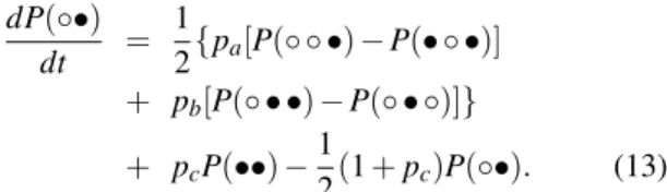
equation forP(•◦)is found dP(◦•)

dt =

1

2{pa[P(◦ ◦ •)−P(• ◦ •)]

+ pb[P(◦ • •)−P(◦ • ◦)]}

+ pcP(••)−

1

2(1+pc)P(◦•). (13) As already mentioned the probabilities of three site clusters appear in the equation. These will be written in terms of two-site probabilities through the so called pair approximation

P(n1n2n3)≈

P(n1n2)P(n2n3) P(n2)

. (14)

Within this approximation, a closed system of two equa-tions is found

dρ

dt = (pa−pb)u−pcρ (15)

du dt =

1 2

·

pa

ru−u2 1−ρ +pb

su−u2 ρ

¸

+ pcs−

1

2(1+pc)u, (16)

whereu≡P(•◦),r≡P(◦◦) =1−ρ−uands≡P(••) =ρ−u. The first equation above corresponds to equation (5), whereas the second is obtained from equation (13) using the pair ap-proximation (14).

The stationary solutions for the densities are ρ=

  

 

0 ifpa<pca

4p2a−4pa+papc+1−pc

4p2

a−4pa+2papc+1−pc otherwise,

(17)

where pc_a= 1

8(4−pc+

p

8pc+p2c). In this approximation

the critical value of pais a function of pc. The critical

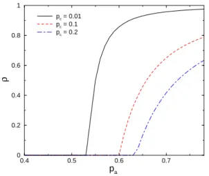
ex-ponents, as expected, have still their mean-field values, only non-universal parameters are different in the two-site approx-imation as compared to the one-site calculation above. Figure (5) showsρas a function of pafor some values of pc in the

two-site approximation.

It may be remarked that in the limitpc→0 both

approxima-tions show a discontinuous transition between two absorbing states, which happens atpa=1/2. In this limit the model

cor-responds to a spin model where a given spin is reversed with a probability proportional to the number of spins in first neigh-bor sites which are in the opposite direction. This might be called a biased voter model whenpais different frompb.

IV. SIMULATIONS

(4)

0.4 0.5 0.6 0.7

p_a

0 0.2 0.4 0.6 0.8 1

ρ

pc = 0.01

pc = 0.1

pc = 0.2

FIG. 5: Density as a function ofpafor some values ofpc, results of

the two-site approximation.

available, and therefore no systematic proof of the existence of the active state may be given, although this was accomplished using probabilistic arguments by Harris in his original work on the contact process [2].

The simulation is done for discrete time, and may be de-scribed by the following steps:

1. Initially, the system ofN sites with periodic boundary conditions is in a state with just one A particle. 2. A list of all sites occupied by A particles is stored, and

at each time step one of them is chosen randomly. 3. Once the site is chosen, a random numberpuniformly

distributed in the interval[0,1]is generated, if p<pa

a B particle is replaced by an A particle in one of the first neighbors, if possible. Otherwise, the A particle at the chosen site will be turned into a B particle either through the spontaneous or through the autocatalytic process.

4. To define the process switching A to B, another random numberqis generated. Ifq<pc/(pb+pc)the change

is spontaneous, otherwise it will happen with a proba-bility proportional to the number of B particles in first neighbors of the chosen site.

5. The time interval associated with the steps above is∆t=

1/NA, whereNAis the number of the sites occupied by

A particles before the step. The process is repeated until either a maximum timetmaxis attained or the absorbing

stateNA=0 is reached.

6. Several runs are done and mean values are calculated as a function of time.

The mean number of A particles, hNAi, as a function of

time for simulations withN=10000 sites,tmax=100000 and

10000 repetitions is displayed in Fig. (6). The number of sites is sufficiently high to ensure that in the simulations the cluster

of A particles is much smaller than the system, thus avoiding finite-size effects in the time interval considered. In a region

1 10 100 1000

t

1 10 100

〈

NA

〉

pa = 0.7 e pc = 0.1

pa = 0.675 e pc = 0.1

pa = 0.6875 e pc = 0.1

FIG. 6: Results of simulations

of the(pa,pc)plane an active state is found for long times in

the simulations. Three curves are shown in Fig. (6). The con-vex one corresponds to an active stationary state, while the concave curve signals that the system will reach the absorb-ing state. These two curves are separated by the third, where a power lawhNAi ∼tθ is seen, corresponding to the critical

condition. We adopt, for all critical exponents, the notation proposed in the review article by Hinrichsen [8].

Repeating simulations in the region (pa+pc≤1), the

crit-ical line may be estimated. The results of these calculations are shown in Fig. (7).

0 0,2 0,4 0,6 0,8 1

p_c

0 0,2 0,4 0,6 0,8 1

pa RI RII

RI : absorbing state RI : active state

S

L. G. M ( T = 0 )

MF1 MF2

CP

FIG. 7: Phase diagram of the model, showing estimates for the tran-sition line between absorbing and active states in the one (MF1) and two (MF2) sites mean field approximations and simulations (S). In

the line pa+pc=1 the model corresponds to the contact process

(CP) and the unbiased voter model (LGM) is recovered at the point

(pa=1/2,pc=0)

(5)

the two-site approximation and, as expected, is situated above the mean field results, which usually overestimate the active region in the parameter space. The value ofλ=pa/(1−pa)at

the critical line attains the limiting valueλc=3.2945±0.0116

aspb→0, in good agreement with the estimated critical value

for the one-dimensional contact processλc=3.29785(2)[12],

as may be appreciated in Fig. (8).

0 0,1 0,2 0,3 0,4 0,5

p_b

1 1,5 2 2,5 3 3,5

λc

FIG. 8: Critical values ofλ=pa/(1−pa)as functions ofpb. The

dashed curve is a fit of a fifth degree polynomial to the points ob-tained in the simulations.

The simulational result forhNAi as a function of time in

the limit of the voter model(pa=1/2,pc=0)is displayed

in Fig. (9). One notices that the initial number of particles is almost conserved, showing a narrow dispersion. This aspect

1 10 100 1000

t

0 1 10

〈

NA

〉

One particle Two particles

FIG. 9: Simulational results for the mean number of A particles as a function of time for the voter model.

may also be appreciated in the histograms shown in Fig. (10), for(pa=1/2,pc=0)and(pa=0.49,pc=0.001), with

ini-tially one A particle. For the voter model a small dispersion is shown around the maximum valuehNAi=1, while in the other

case the maximum is shifted to the absorbing statehNAi=0

0.1 0.2 0.3 0.4 0.5 0.6 0.7 0.8 0.9 1 1.1 1.2

0 5000 10000 15000

0.1 0.2 0.3 0.4 0.5 0.6 0.7 0.8 0.9 1

〈NA〉

0 1000 2000 3000 4000 5000

FIG. 10: Histograms of the mean number of A particles. The upper

figure corresponds to the voter model (pa=1/2,pc=0) and the

other figure is for a point of the parameter space close to the voter model (pa=0.49,pc=0.001) where the absorbing statehNAi=0 is

stable.

The simulations allow us to follow the dynamic evolution of mean values that describe the model, such as the mean num-ber of A particles hNA(t)i, the probability of survival Ps(t)

that at the timet at least one particle A is present in the sys-tem and the mean square radiusR2(t) =h∑ii2ηi(t)i/hNA(t)i.

These variables satisfy the following scaling forms at the crit-ical point [4]:

hNAi(t) ∼ tθ,

Ps(t) ∼ t−δ,

R2(t) ∼ t2/z. (18) Through scaling and hyperscaling relations, these critical ex-ponents define all other exex-ponents of the model, and thus their values identify the universality class.

-0,25 -0,2 -0,15 -0,1

−δ

0,29 0,3 0,31 0,32 0,33

θ

0,02 0,04 0,06 0,08 0,1 0,12 0,14 0,16 0,18 0,2 0,22

p_c

1 1,05 1,1 1,15 1,2 1,25 1,3

2/z

FIG. 11: Dynamical critical exponents as functions of the rate pc.

The dashed lines indicate the values of these exponents for the CP.

(6)

shown in Fig. (11). For most of the values for pc,

particu-larly those close to the CP (pc≈0.2327), the estimated

expo-nents are close to the values known for the CP (θ=0.313686, δ=0.159464, and 2/z=1.265226 [13]). The relative er-rors are displayed in Fig. (12). Also, the hyperscaling rela-tion 2d/z=4δ+2θis satisfied numerically with some im-precision, as may be seen in Fig. (13). Some systematic er-ror seems to be present in the estimates for the mean square radius, which propagates to the hyperscaling relation verifi-cation. As pc→0, however, when the voter model is

ap-proached, a departure of all estimates from the CP values is apparent.

0 0,1 0,2 0,3 0,4 0,5 εδ

0 0,05 0,1 0,15 0,2

ε θ

0,02 0,04 0,06 0,08 0,1 0,12 0,14 0,16 0,18 0,2 0,22

p_c

0 0,5 1 1,5 2

ε2/z

FIG. 12: Relative errors of the estimates of dynamical critical expo-nents compared to the CP values.

0 0,02 0,04 0,06 0,08 0,1 0,12 0,14 0,16 0,18 0,2 0,22

p_c

-1 -0,8 -0,6 -0,4 -0,2 0

2d/z-4

δ

-2

θ

FIG. 13: Verification of the hyperscaling relation for the dynamical critical exponents.

For models with a discontinuous transition with a spin in-version symmetry, such as the voter model, the dynamic crit-ical exponents are given byθs=0,δs=1/2 e 2/zs=1 and

the hyperscaling relation is given byδs+θs=d/zs,

corre-sponding to the compact directed percolation (CDP) univer-sality class [8]. An analysis of the exponents in the limit pc→0 may be performed fitting a cubic curve to the

esti-mates, as is shown in Fig. (14) for the exponentδ. The values

0 0,001 0,002 0,003 0,004 0,005 0,006 0,007 0,008 0,009 0,01

p_c

-0,4 -0,38 -0,36 -0,34 -0,32 -0,3 -0,28 -0,26

−δ

FIG. 14: Limit forpc=0 of the dynamical exponentδ.

obtained through this procedure areδ=0.44,θ=0.07, and 2/z=1.01, which are not far from the known values given above. The variation of the estimates for critical exponents with the parameters of the model close topc=0 is probably

an apparent effect, due to large fluctuations observed in the simulations in this region, and the whole critical line, with ex-ception of the terminal voter model point, is in the same uni-versality class of the CP, as suggested by the DP conjecture. This situation is quite similar to what is observed in the be-havior of the Domany-Kinzel probabilistic cellular automaton (DKPCA) [14], which in a line of its phase diagram corre-sponds to the CP with discrete time and parallel update, and also exhibits a crossover from the DP to the compact direct percolation (CDP) universality class [15]. It is believed, al-though to our knowledge not proven, that changing the update process in a stochastic model may affect non-universal quan-tities only. The pointpa=1/2,pc=0 may be recognized as

a multicritical point, and in its neighborhood any stationary density variable should exhibit the scaling form

g(pa−1/2,pc)∼(pa−1/2)egF

µ _p

c

[pa−1/2]φ ¶

. (19)

The critical exponent associated with the density variableg, eg, should correspond to the CDP universality class, and the

scaling functionF(z)is singular at a valuez0of its argument, which corresponds to the critical line. Thus, the critical line is asymptotically given bypc=z0(pa−1/2)φand the amplitude

(7)

V. NUMERICAL DIAGONALIZATION

Another approach to study 1+1 dimensional stochastic sys-tems is the exact solution of models with increasing numbers of sites N followed by extrapolations to the thermodynamic limit [8]. This is accomplished writing the master equation (1) as

∂

∂t|P(t)i=

S

ˆ|P(t)i, (20) where ˆ

S

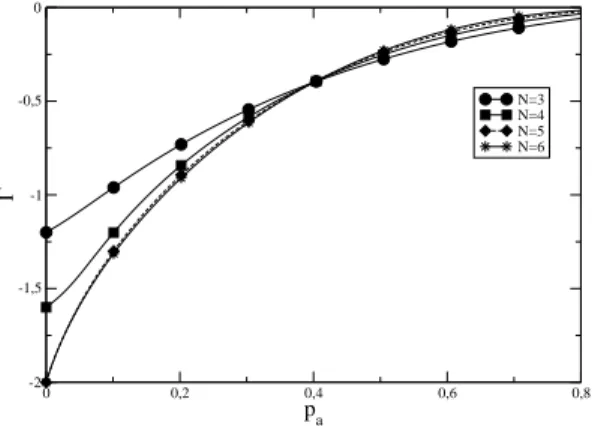
_{is the time evolution operator of the model. In the} representation in which it is diagonal, vanishing eigenvalues µ0=0 correspond to stationary states of the system. For finite systems with absorbing states, only these states are stationary, and no active stationary state is found.

To study the transition between an active and a stationary state, we may consider the behavior of the eigenvalue with the second smallest absolute valueΓ≡µ1of the operator ˆ

S

_{. This} eigenvalue is related to the quasi-stationary [17] state and will eventually become degenerate withµ0in the thermodynamic limit, originating the phase transition. Figure (15) shows the behavior of the gapΓfor some values of the sizeN. For a

0 0,2 0,4 0,6 0,8

p_a

-2 -1,5 -1 -0,5 0

Γ

N=3 N=4 N=5 N=6

FIG. 15: GapΓas a function of pafor system sizesN=3,4,5,6

withpc=0.2.

fixed value ofpc. the finite size scaling behavior of the gapΓ

is given by [8]

Γ=N−zf(|pa−pc_a|N1/ν⊥₎_, ₍₂₁₎ where pc_ais the critical value of pafor a fixed value of pc.

Defining the quantity

YN(pa,pc) =

ln[Γ(pa,pc;N+1)/Γ(pa,pc;N−1)]

ln[(N+1)/(N−1)] , (22)

we may estimate the critical point pc_a(N) finding the inter-section of the curvesYN andYN+1[18]. This procedure re-sembles the phenomenological renormalization group. The sequence pc_a(N)of estimates for a given value of pc, with

N=4,5, . . .M, was extrapolated to the thermodynamic limit

N→∞using the BST algorithm [19], which even for the lim-ited number of estimates considered lead to rather precise re-sults. Figure (16) shows the extrapolated estimates for the

0 0,02 0,04 0,06 0,08 0,1 0,12 0,14 0,16 0,18 0,2 0,22

p_c

0,5 0,55 0,6 0,65 0,7 0,75

pa

FIG. 16: The squares are the extrapolated estimates obtained from the numerical diagonalization results, compared with the critical lines resulting from simulations (full line) and the two-site approxi-mation (broken line).

critical line, compared with the results provided by the simu-lations and the two-site approximation results. The agreement between the simulation and the present results is apparent. The results for the critical line close to the CP pointp_b=0 were extrapolated to the CP limit using a cubic function and the resulting value wasλc=3.3081±0.0173, which is in

rea-sonable agreement with a more precise estimate in the litera-tureλc=3.29785(2)[12]. We also estimate the crossover

ex-ponentφ, through a fit to the critical line in the neighborhood of the voter model limit and it is results inφ=2.24±0.07.

Once the extrapolated estimates for the critical line were obtained, the critical exponents z andξ=z−1/ν⊥may be estimated using the asymptotic scaling forms

Γ(pa,pc) ∼ L−z

∂ ∂pa

Γ(pa,pc) ∼ L−ξ, (23)

for a fixed value ofpcand pa=pca, on the critical line. An

estimate of the exponents is obtained for each size of the sys-tem, and the estimates are extrapolated to the thermodynamic limit. Our results for these two static exponents are shown in Fig. (17).

Again a departure of the estimates from the CP values may be observed aspcbecomes smaller. The CDP values for these

exponents arezs=2 andξs=1. Unlike to what was observed

in the simulations no systematic trend to these values was ob-served in the estimates from exact diagonalization aspc→0.

We noticed, even considering values ofNup to 15, that aspc

(8)

0 0,05 0,1 0,15 0,2 1,3

1,4 1,5 1,6 1,7 1,8

z

0 0,02 0,04 0,06 0,08 0,1 0,12 0,14 0,16 0,18 0,2 0,22

p_c

0,4 0,5 0,6 0,7 0,8

ξ

FIG. 17: Static exponents estimated through the exact diagonaliza-tion for finite systems. The values for the CP are shown in dashed lines.

VI. CONCLUSION

We discussed the transition between an absorbing (ρ=0) and an active (ρ>0) steady states in a stochastic model of interacting particles. This model displays a line of continuous transition between these states starting at a point which cor-responds to the contact process and ends at a point where the model is equivalent to the voter model, showing a discontin-uous transition between two absorbing states. The phase dia-gram thus obtained is similar to what is found in a problem of equilibrium polymerization in a grand-canonical ensemble on an anisotropic square lattice [20], where the polymer is mod-eled as a self-avoiding walk and the activity of a horizontal link is equal toxand a vertical link is associated with an ac-tivityy. A continuous transition is observed in general in the

(x,y)plane, between a non-polymerized (ρ=0) and a poly-merized (ρ>0), whereρcorresponds to the fraction of lattice sites visited by the walk. However, atx=0 ory=0 the walk is

one-dimensional, and a discontinuous transition is found be-tween the non-polymerized and the fully polymerized (ρ=1) phases [21].

The localization of the critical line in the parameter space of the model was found in the one- and two-site approximations, as well as through simulations and numerical diagonalization of the time evolution operator. The evidences obtained from estimates of critical exponents suggest that the whole critical line belongs to the DP universality class, and a crossover to the CDP universality class is observed at the terminal voter model point. From the estimates for the location of the criti-cal line close to the voter model point the crossover exponent φ=1.80±0.03 was obtained. Although the estimated value for φis smaller than the mean-field result φ=2, the latter is inside the confidence interval of the estimate, so that it is not possible to decide if the crossover exponent has a non-classical value. Due to the difficulties we had with the simu-lations and the numerical diagonalization in the multicritical region, we suspect that another approach is necessary to clear this point. We are presently addressing this point through a series expansion approach. Another extension of this work would be the study of the crossover between the universality class in the Domany-Kinzel cellular automaton, which corre-sponds to the CP with parallel update in a subspace of its pa-rameter space and also has a point of its phase diagram which corresponds to the voter model.

Acknowledgments

We thank Prof. Ronald Dickman for many helpful dis-cussions and a critical reading of the manuscript. This research was partially supported by the Brazilian agencies CAPES, CNPq and FAPERJ, particularly through the project PRONEX-CNPq-FAPERJ/171.168-2003.

[1] J. Marro and R. Dickman,Nonequilibrium Phase Transitions

in Lattice Models (Cambridge University Press, Cambridge, 1999)

[2] T.E. Harris,Ann. Probab.2, 969 (1974).

[3] F. Schl¨ogl,Z. Phys.253, 147 (1972).

[4] P. Grassberger and A. De La Torre,Ann.Phys.122, 373 (1979).

[5] R. M. Ziff, E. Gulari, and Y. Barshad,Phys. Rev. Lett.56, 2553

(1986).

[6] H. Takayasu, A. Tretyakov, and A. Yu,Phys. Rev. Lett.68, 3060

(1992).

[7] H. K. Janssen,Z. Phys. B,42, 151 (1981); P. Grassberger, Z.

Phys. B,47, 365 (1982).

[8] H. Hinrichsen,Adv. Phys.49, 815 (2000).