422 Brazilian Journal of Physics, vol. 34, no. 2A, June, 2004
Kinetic Phase Transition in the Mixed-Spin Ising Model
M. Godoy and W. Figueiredo
Departamento de F´ısica, Universidade Federal de Santa Catarina, 88040-900, Florian´opolis, SC, Brazil
Received on 9 August, 2003
In this work we studied a ferromagnetic mixed-spin Ising model including a single ion crystal-field term. The model system consists of two interpenetrating sublattices with spinsσ= 1/2andS = 1. The spinsσ= 1/2
occupy the sites of one sublattice, their nearest-neighbours are spinsSon the other sublattice, and vice versa. The system is in contact with a heat bath, the spins flipping according to the Metropolis transition rate and, at the same time, subject to an external flow of energy, which is simulated by a two-spin flip process. The model is studied via the dynamical pair approximation and through Monte Carlo simulations. We have determined the phase diagram of the model in the plane crystal-fieldDversus competition parameterp. The parameterp
accounts for the competition between the one- and two-spin flip processes. In the pair approximation, the phase diagram, at high temperatures, present three phases separated by two transition lines: a continuous transition line between the ferromagnetic and paramagnetic phases, and a first-order transition line between the paramag-netic and antiferromagparamag-netic phases. However, Monte Carlo simulations predict the same topology for the phase diagram as the pair approximation, but all the transition lines are continuous for any value of the temperature.
The mixed-spin Ising model has received much atten-tion in the last years. The main motivaatten-tion is that the model, containing spins of different magnitudes, is used to under-stand the behavior of certain ferrimagnetic systems that are of great technological interest. From a theoretical point of view many different approaches have been employed in the study of this model: effective-field theories with correla-tions [1, 2], the mean-field renormalization group [3, 4], the Bethe-Peierls method [5], and Monte Carlo simulations [7, 6]. In these studies, just the equilibrium states were in-vestigated.
In the study of the stationary states of the nonequilib-rium thermodynamic systems we do not have at our dis-posal a closed formalism to deal with these systems as in the equilibrium problems [8, 9]. In this work we shall con-sider a mixed-spin Ising model defined on a square lattice, with spins σ = 1/2 andS = 1. The lattice is divided into two interpenetrating sublattices, with the σ spins oc-cupying the sites of one sublattice, while the S spins oc-cupy the sites of the other sublattice, each sublattice con-taining N sites. A state of the system is represented by (σ, S) ≡ (σ1, ..., σj, ..., σN;S1, ..., Si, ..., SN), where the
spin variables σj can assume the values±1, and the spin
variablesSiassume values±1and0. The system is
repre-sented by the following hamiltonian model
H=−J
i,j
Siσj−D
i
S2
i , (1)
where the sum is over all nearest neighboring pairs of spins.
J is the coupling constant between nearest neighbors spins andDis the crystal-field contribution.
Let us callp(σ, S;t)the probability of finding the sys-tem in the state(σ, S)at timet. The equations of motion
for the probability of the states of the system is given by the master equation
d
dtp(σ, S;t) =−
σ′,S′
W(σ, S→σ′, S′)p(σ, S;t)
+
σ′,S′
W(σ′, S′→σ, S)p(σ′, S′;t), (2)
where W(σ, S → σ′, S′) is the probability, per unit of
time, for the transition from the state (σ, S) to the state (σ′, S′). In this model, we assumed that the transition rate
W(σ, S → σ′, S′)is due to the competition between two
independent stochastic processes. First, the one-spin flip Glauber process [10], intended to describe the relaxation of the spinsσandSin contact with the heat bath. This transi-tion rate can be written as
WG(σ, S→σ′, S′) = WG(σ, S→σ′, S)
+WG(σ, S→σ, S′). (3)
Second, the two-spin flip process, chosen to be independent of temperature, and meant to increase the energy of the sys-tem, can be written asWGD(σ, S→σ′, S′). Then, we have
the following equation for the total transition probability:
W(σ, S→σ′, S′) =pW
G(σ, S→σ′, S′)
+(1−p)WGD(σ, S→σ′, S′), (4)
where0≤p≤1is the competition parameter between the one- and two-spin flip processes. From the master equation we found the equations of motion for the sublattice magne-tizationsm1=σjandm2=Si, and also for the
corre-lation functionsq=
S2
i
,q1 =
σjSi2
andr=σjSias
M. Godoy and W. Figueiredo 423
These mean values are calculated using the following transition rates: for the one-spin flip transition rate, which simulates the contact of the system with the heat bath, we used the Metropolis prescription, given by
ωj(σ) = min[1,exp(−β∆Ej)], (5)
whereβ = 1/kBT, andT is the absolute temperature of
the heat bath.∆Ejis the change in energy after flipping the
spinσj at sitej. We also assumed a similar expression for
ωi(S). On the other hand, for the two-spin flip transition
rate, which favors the increase of the energy of the system, we chose the following rule
ωij(S, σ) =
0 if ∆Eij ≤0
1 if ∆Eij >0, (6)
where∆Eijis the change in energy after flipping the spins
Siandσj, at the neighboring sitesiandj.
In the present study of this model we used the dynam-ical pair approximation and Monte Carlo simulations. The set of equations of motion obtained from the master equa-tion can be solved through the dynamical pair approxima-tion [11], and the steady states of the system can be found as a function ofT,pandD. The equations are solved numer-ically by employing the fourth-order Runge-Kutta method. The solutions and the corresponding phases are defined in the following way: ferromagnetic phase (F), m1 = m2,
m1 and m2 having the same signs; paramagnetic phase
(P),m1 = m2 = 0; antiferromagnetic phase (AF), where
m1=m2,m1andm2having different signs.
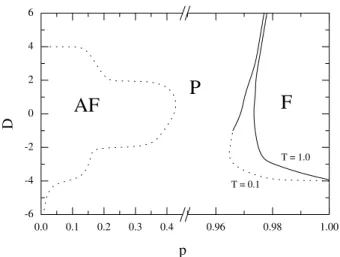
We present in Fig. 1, the phase diagram of the model in the plane crystal-field intensity D versus competition parameter p, for two selected values of temperature. For these temperatures, the phase diagram displays three differ-ent phases separated by differdiffer-ent transition lines. For the values ofpin the range1≥p0.96, andD >−4.0J, the phase diagram presents only a ferromagnetic phase (F). At low temperatures,T = 0.1J in Fig. 1, the continuous line changes into a first-order line for negative values ofD. The transition between the ferromagnetic (F) and paramagnetic (P) phases exhibits a tricritical point. Increasing the tem-perature beyondT = 0.262J the tricritical behavior disap-pears. The area occupied by the ferromagnetic phase (F) in-creases when the temperature dein-creases. On the other hand, for small values ofp, what corresponds to a large flow of energy into the system, the phase diagram presents the anti-ferromagnetic (AF) and paramagnetic (P) phases, which are separated by a first-order transition line. For this model, this transition line is almost independent of temperature.
0.0 0.1 0.2 0.3 0.4 0.96 0.98 1.00 -6
-4 -2 0 2 4 6
T = 0.1 T = 1.0
F
AF
P
D
p
Figure 1. Phase diagram in the plane crystal-fieldDvs competi-tion parameterp, for two selected temperatures, in the dynamic pair approximation. The letters F, AF and P, denote ferromagnetic, an-tiferromagnetic and paramagnetic phases, respectively. The solid lines represent continuous phase transitions, and the dashed lines are the first-order transition points. The temperatures are indicated in the figure.
We also performed Monte Carlo simulations for this model, in order to get a better understanding of the phase transitions found from the pair approximation calculations. We considered a square lattice of linear sizeL, withL rang-ing from L = 16 toL = 128, and we applied periodic boundary conditions. For each simulation run, the initial states of the system were completely random. A new con-figuration is generated by the following Markov process: for selected values of the temperatureT, crystal-field intensity
D, and the competition parameter p, we choose a spin at random on the lattice, and we generate a random numberξ
between zero and one. Ifξ≤pwe considered the one-spin flip process, according to the heat bath algorithm. On the other hand, ifξ > p, then we consider the two-spin flip pro-cess. In this case, we randomly select another spin, which is a nearest neighbor of the initial spin, and then the state of the system is changed only if energy increases. We dis-carded the initial5×104MCS (Monte Carlo steps) until the
system enters in a stationary regime. Then, we used more 5×10⁴MCS to calculate the averages of the quantities of
interest. One MCS corresponds toL2one- and two-spin flip
trials.
We calculated the sublattice magnetization per spin,
m1 = N1
iSiandm2 = N1
jσj
. The transition lines of the phase diagram were obtained from the total and staggered magnetizations, defined asmF
L = 12|(m1+m2)|
andmAF
L =12|(m1−m2)|, respectively. We also calculated
the reduced fourth-order Binder cumulants associated with these magnetizations. From the crossing point of the cu-mulants for different lattice sizes we determined the critical points of the model.
dif-424 Brazilian Journal of Physics, vol. 34, no. 2A, June, 2004
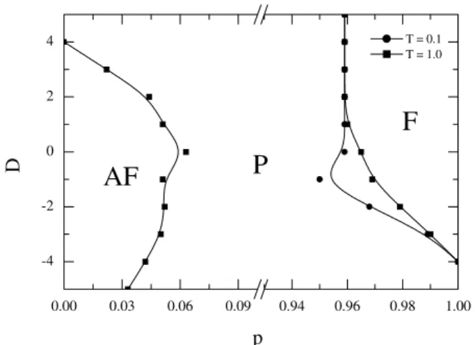
ferent phases observed in Fig. 1. However, in the Monte Carlo simulations, all the transition lines are continuous, and no tricritical point is observed. For large values of p
(0.95 ≤ p ≤ 1.0) andD ≥ −4J, Fig. 2 shows only a ferromagnetic phase (F). The area occupied by this phase also decreases for increasing values of the temperature. On the other hand, the antiferromagnetic phase appears only for very small values ofp. In Fig. 2 we see that it is restricted to 0.0≤p≤0.06region. Compared with the phase diagram obtained in the context of the pair approximation, we note that the paramagnetic phase (P) occupies a very large area.
-4 -2 0 2 4
0.00 0.03 0.06 0.09 0.94 0.96 0.98 1.00
T = 0.1 T = 1.0
AF
P
F
p
D
Figure 2. Phase diagram in the plane crystal-fieldDvs competition parameterp, from Monte Carlo simulations, for two selected tem-peratures, as indicated in the figure. The letters F, AF and P, denote the ferromagnetic, antiferromagnetic and paramagnetic phases, re-spectively. The lines joining the squares and the circles represent continuous transition lines.
This work was partially supported by the Brazilian agen-cies CAPES, CNPq and FUNCITEC(SC).
References
[1] T. Kaneyoshi, Solid State Communc.70, 975 (1989); Physica A205, 677 (1994).
[2] A. L. de Lima, B. D. Stoˇso´c, and I. F. Fittipaldi, J. Magn. Magn. Mater.226, 635 (2001).
[3] J. A. Plascak, W. Figueiredo, and B. C. S. Grandi, Braz. J. Phys.29, 579 (1999).
[4] H. F. V. de Resende, F. C. S´a Barreto, and J. A. Plascak, Phys-ica A149, 606 (1988).
[5] T. Iwashita and N. Uryu, J. Phys. Soc. Jpn.53, 721 (1984).
[6] G. M. Buendia, M. A. Novotny, and J. Zhang, in: D. P. Lan-dau, K. K. Mon and H. B. Schttler (EDS.), Springer Proceeds in Physics, Vol., 78, Computer Simulations in Condensed Matter Physics VII, Springer, Heidelberg, 1994, p. 223.
[7] G. M. Buendia and M. A. Novotny, J. Phys.: Condens. Mat-ter.9, 5951 (1997).
[8] J. Marro and R. Dickman,Nonequilibrium Phase Transitions in Lattice Models(Cambridge University Press, Cambridge, 1999).
[9] V. Privman, ed., Nonequilibrium Statistical Mechanics in One Dimension (Cambridge University Press, Cambridge, 1996).
[10] R. J. Glauber, J. Math. Phys.4, 294 (1963).