SPATIAL PATTERN RECOGNITION OF EXTREME TEMPERATURE CLIMATOLOGY:
ASSESSING HadCM3 SIMULATIONS
VIA
NCEP REANALYSES OVER EUROPE
P. S. LUCIO
1, 2, F. C. CONDE
1, 3& A. M. RAMOS
11
Centro de Geofísica de Évora (CGE), Évora, Portugal.
2
Universidade Federal do Rio Grande do Norte (UFRN), Natal - RN, Brasil.
3
Instituto Nacional de Meteorologia (INMET/CDP), Brasília - DF, Brasil.
e-mails:
1[email protected];
3[email protected];
1[email protected]
2
Corresponding author: Paulo Sérgio Lucio
Departamento de Estatística - CCET - UFRN - Lagoa Nova – Natal-RN - CEP 59.072-970
e-mails:
2[email protected]
Received October 2005 - Accepted May 2006
ABSTRACT
This article attempts to quantify the spatial uncertainties associated with extreme temperature’s response, by assessing data derived from climate model. This is undertaken by a comparison of the spatial pattern of a long-term time-series aggregation (1960/61–1989/90) for extreme temperatures simulated by a particular GCM (the UK Met Offi ce - Hadley Centre climate model, HadCM3) to that of the USA NCAR NCEP Reanalyses, which are considered as ‘truth’, over the MICE (Modelling the Impacts of Climate Extremes - EU Project) spatial domain. Since evaluation of models is crucial to assessing future scenarios, the aim of this study is to investigate whether the extreme values predicted by the HadCM3 climate model can simulate those produced by NCEP Reanalyses, assuming that the extremes of both models are realizations of the same spatial stochastic process. To get more useful information about the uncertainties surrounding spatial climate projection, one also has to analyze the pattern of temperature extremes in terms of their anomalies. A common technical issue in the assessment of numerical spatial models is based on the Principal Components Analysis and Bayesian Classifi cation for spatial pattern recognition. These methodologies are very important and useful for guiding an evolutionary statistical model-building process. This study leads to the conclusion that the HadCM3 Simulations do not realistically reproduce the NCEP Reanalyses, despite the fact that the climatology of extremes has demonstrated very similar spatial patterns. It is likely therefore that such instability may persist in the future.
Keywords: anomaly, empirical Bayesian classification; compositing; principal components
loading.
RESUMO: ANÁLISE DO PADRÃO ESPACIAL DA CLIMATOLOGIA DE TEMPERATURAS
EXTREMAS: AVALIANDO SIMULAÇÕES DO HADCM3 VIA REANÁLISES DO NCEP PARA A EUROPA.
1. INTRODUCTION
The purpose of this manuscript is to evaluate the spatial ability of a GCM output to reproduce the present-day occurrence of temperature extremes over the European geographical domain. Basically, one would like to confi rm whether, stochastically and visually, the spatiotemporal aggregated extreme patterns (long-term climate signal) obtained from the HadCM3 Simulations can be considered as realizations of the NCEP Reanalyses. To evaluate the hypothesis of model performance one uses a straightforward interpolation rescaling followed by Principal Components Analysis and Bayesian Classification – two alternative methods to corroborate the results in Lucio, 2004a and Lucio, 2004b).
Since the high risk of getting the wrong strategy decision concerning future scenarios and impacts has costly economic and social consequences. Hypothesis on climate change concerning global climate models can be rejected through comparison with observations or reanalyses database, but improbably confi rmed. Assessments (Fuentes et al., 2003) of GCM simulation models by statistical techniques have been historically concentrated mainly on monthly and seasonal means. Considering extreme measures of climate models and reanalyses studies, the spatial prognostic of large-scale is an important component. The failure to neglecting this spatial information (Lucio, 2004a; Lucio, 2004b) can lead to errors in decision-make.
Hence, basically, one would like to confi rm whether stochastically the long-time aggregated extreme values obtained from the HadCM3 Simulations can be considered realisations of the NCEP Reanalyses over the MICE (Modelling the Impacts of Climate Extremes: MICE EVK2-CT-2001-00118 - European Research Project) geographical domain. For this reason, the climatology and the anomaly spatial patterns from the HadCM3 Simulations are compared with the corresponding ones from the NCEP Reanalyses, in the same spatial domain.
2. EXPERIMENTAL DATASET
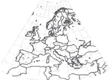
Climate scenarios are defi ned by particular climate forcing in the dynamical simulations of climate models. The general circulation models (GCM) are the most complex of these models and such the most powerful tools available for making realistic estimates of climate change. However, they involve much uncertainty, especially in terms of estimating regional or local change essentially with reference to the extremes. In this work, the spatial pattern of extreme temperature climatology and anomaly over the MICE spatial domain (Figure 1) are analysed to assess the output of the HadCM3 Simulations and the NCEP Reanalyses.
Figure 1 – The geographical domain to assess HadCM3
Simulations from NCEP Reanalyses. HadCM3 (GCM Model): 16long × 19lat = 304pts, 15◦W - 41.25◦E, 30◦N - 75◦N; NCEP (Reanalyses): 31long × 25lat = 775pts, 15◦W - 41.25◦E, 29.52◦N - 75.24◦N.
The HadCM3 Simulation is performed with a coupled atmosphere-ocean general circulation model (AOGCM) developed at the Hadley Centre - UK and described by incertezas acerca da projeção espacial de clima, deve-se também analisar o padrão de extremos de
temperatura em termos de suas anomalias. Uma técnica comum na avaliação de modelos numéricos está baseada na Análise de Componentes Principais ou na Classifi cação Bayesiana Empírica para o reconhecimento do padrão espacial. Estas metodologias são muito importante e úteis para guiar o processo de estatístico evolutivo na construção de modelos. Este estudo conduz à conclusão que as simulações do HadCM3 não reproduzem realisticamente as reanálises do NCEP, apesar da climatologia de extremos ter demonstrado padrões espaciais semelhantes. É provável, então, que tal instabilidade possa persistir no futuro.
Palavras-chave: anomalia, classifi cação Bayesiana empírica; “compositing”; “loadings” das
Gordon et al. (2000) and Pope et al. (2000). The HadCM3 model produces values for grid squares over a temporal window. The NCEP/NCAR Reanalyses (National Center for Environmental Prediction/National Center of Atmospheric Research - USA), which are currently available back to 1948, contain several meteorological parameters in a global spatial resolution of 2.5° x 2.5° (latitude x longitude) and in a vertical extent from the surface up to 10 hPa level, c.f. Kalnay et al. (1996). The spatial window for HadCM3 covering the MICEdomain is a regular grid with 2.5° latitude by 3.75° longitude (16 long x 19 lat = 304 points) and for the NCEP Reanalyses is represented with a Gaussian grid, which preserves equal areas, spaced of 1.875° longitude by 1.903801° latitude (31 long x 25 lat = 775 points).
The elementary dataset under study consists on the temporal aggregated coldest and warmest temperatures from winter (December, January and February - DJF) and summer (June, July and August - JJA) assembled. The climatology was calculated separately for each grid point as the average value (calculated over the period of record: 1960/61–1989/90). Hence, the climatology for nocturnal and diurnal extreme temperatures were calculated based on the 30 recorded years subdivided into the four following work-ensembles:
1. Spatial climatology of the winter coldest minimum temperature (TMIN.W);
2. Spatial climatology of the winter warmest maximum temperature (TMAX.W);
3. Spatial climatology of the summer coldest minimum temperature (TMIN.S);
4. Spatial climatology of the summer warmest maximum temperature (TMAX.S).
These marks were chosen because they represent the warmest and coldest days/nights, related to the winter and summer seasons. Furthermore, the dependence of temperature extremes on geographical attributes was considered, since the extreme temperature depends on the latitude (solar forcing), altitude, and contrasts land-water and land-topography - both spatial patterns are expected to be very similar, which can be predictable by a simple spatial autoregression moving average interpolation.
In practice, to get large-scale comprehensible information, it is more useful to analyse meteorological extremes considering their anomalies (δ): the deviation of the absolute extreme measure from the long-term average value (i.e., the deviation of the coldest or the warmest temperature for a year from the long-term average value of the coldest or the warmest daily temperature). The reason for using anomalies is to attempt to remove the infl uence of latitude, longitude, and land/ocean differences. Hence, the anomalies were calculated separately for
each grid point as the difference between the largest maximum (smallest minimum) temperature for a particular season and year and the average value (calculated over the period of record) of the largest maximum (smallest minimum) temperature at that grid point. Hence, the anomalies for minimum and maximum extreme temperature events were calculated based on the 30 recorded years subdivided into the four following work-ensembles:
1. Spatial anomalies of the winter minimum temperature
(δTMIN.W);
2. Spatial anomalies of the winter maximum temperature
(δTMAX.W);
3. Spatial anomalies of the summer minimum temperature
(δTMIN.S);
4. Spatial anomalies of the winter maximum temperature
(δTMAX.S).
The NCEP Reanalyses are obtained at individual centred-grid points and have different spatial resolution from the HadCM3 Model output. Consequently, it is not straightforward to compare NCEP Reanalyses to the HadCM3 Model output directly. Rather, some “regriding” or rescaling of the data, by means a spatial interpolation is needed for comparability. This requires a statistical procedure with adequate precision, such as the compositing interpolation onto a common grid (Kysely, 2002a; Kysely, 2002b). The basic idea of the statistical rescaling (compositing or changing of support) to assess spatial information is to project an empirical large-scale spatial variable on a different space-domain (Cressie, 1996). This technique is based on the assumption that all small-scale variability can be explained or recovered from large-small-scale variability (von Storch, 1999).
3. DATA REGRIDING
A two-dimensional spatial process can be characterized by a simple realisation of a stochastic model {δT(s) : s ∈ ℜ2} where s ∈ ℜ2 represent a generic data location. The trend surface model is a polynomial based on data location, which summarizes the dependence of the response variable {δT(s) : s ∈ ℜ2} on the explanatory factors {s = (x, y) ∈ ℜ2} and occasionally some factors that has distinct levels, in the vein of {ocean/sea, land} dummy variables (Draper and Smith, 1998), in order to take into account that this information may have separate deterministic effects on the extreme temperature anomalies, by the trend surface stochastic equation (Cressie, 1996; Bailey and Gatrell, 1996).
used to identify, explore and characterize the effect of potential large-scale factors on an outcome variable is the compositing (compositing refers to creating solutions by combining objects from different sources). The main advantage of this method is its simplicity in both implementation and understanding. It is extremely fl exible, able to capture both localized and moving features and to quantify non-linearity in the behavior (by comparing opposite phases of the extreme events).
In this work one interpolates through the data points by polynomials cubic splines to determine the predicted extreme anomalies ({δT(s) : s ∈ ℜ2}) - For n given points there exists a unique polynomial of degree n-1 or less which passes through these points. A cubic spline is a piecewise cubic polynomial such that the function, its derivative and its second derivative are continuous at the interpolation nodes. The natural cubic
spline has zero second derivatives at the endpoints. It is the smoothest of all possible interpolating curves in the sense that it minimizes the integral of the square of the second derivative (de Boor, 1978).
The spatial similarities between both models are illustrated in Figure 2a-b and Figure 3a-b, where signifi cant spatial misfi ts are locally detected essentially vis-à-vis of the minimum temperature systems (Figure 2a and Figure 3a). The
differences are largely infl uenced by topography, latitudinal heat and energy balances. The compositing method involves constructing an indicator which correlates with the variability of the phenomenon of interest. Making a regression of the “index” onto the data yields composite spatial patterns of variability.
A potential problem with climate data is that they undoubtedly present a spatial-dependence component; it can result in spatial autocorrelation which causes nuisances for statistical methods that make assumptions about the independence of residuals. Tests to detect spatial autocorrelation can be performed as an exploratory technique to decide whether results from spatial regression modeling could be used. If spatial residual autocorrelation exists it will violate the assumption about the independence of residuals and the validity of hypothesis testing in model fi t is questioned. The main effect of such violations is that the residual squared sum is underestimated, infl ating the value of test statistic that increases the chance of a Type I error - incorrect rejection of the null hypothesis, H0:
no spatial autocorrelation. Hence, in attributes motivating the spatial pattern of the residual analyses, the level, the nature and strength of the interdependence intrinsic to each temperature extreme ensemble were defi ned by a measure of residuals spatial association, the Moran’s indices (Moran, 1948).
Figure 2 – Spatial bivariate interpolation of the (a, b) winter and (c, d) summer maximum TMIN extreme temperatures.
The isotherms designed from the 30-years climatology for both models the (a, c) HadCM3 Simulations and the (b, d) NCEP Reanalyses.
-3*10^6 -2*10^6 -10^6 0 10^6 2*10^6 3*10^6
-2*10^6
-10^6
0
10^6
2*10^6
0
0 5
5
5 5
5 10
10
10
10
10 1015
15 15
15 15
20
20 20
25 25
25
30 30
30 30
-3*10^6 -2*10^6 -10^6 0 10^6 2*10^6 3*10^6
-2*
10^
6
-10^
6
0
10^
6
2*
10^
6
-10 -5
-5 -5
0
5
5 5
5
5
10
10
10
10
10 15
15
15
15
-3*10^6 -2*10^6 -10^6 0 10^6 2*10^6 3*10^6
-2*
10^
6
-10^
6
0
10^
6
2*
10^
6
10
10 10
20
20
30
30
40 40
40
40 40
40
40 40 50
-3*10^6 -2*10^6 -10^6 0 10^6 2*10^6 3*10^6
-2*
10^
6
-10^
6
0
10^
6
2*
10^
6 10
20
20 20
30
30 30
30
40
40
40 40
40 50
5050 50
HadCM3 Simulations
Extreme Temperature Climatology - TMIN.S Extreme Temperature Climatology - TMIN.SNCEP Reanalyses
a) b)
HadCM3 Simulations
Extreme Temperature Climatology - TMAX.S Extreme Temperature Climatology - TMAX.SNCEP Reanalyses
-3*10^6 -2*10^6 -10^6 0 10^6 2*10^6 3*10^6
-2*
10^
6
-10^
6
0
10^
6
2*
10^
6
-60 -60
-60
-40 -20
-20
-20
-20
-20 -20
-20
0
0
-3*10^6 -2*10^6 -10^6 0 10^6 2*10^6 3*10^6
-2*
10^
6
-10^
6
0
10^
6
2*
10^
6
-50 -40
-40 -40
-40 -30
-30
-30
-30 -20
-20 -20
-20
-10 -10
-10 -10 -10
-10
-10
0
0 0 10
-3*10^6 -2*10^6 -10^6 0 10^6 2*10^6 3*10^6
-2*
10^
6
-10^
6
0
10^
6
2*
10^
6
0
5 10
10
10
15 15
15
15
20 20
20
25
-3*10^6 -2*10^6 -10^6 0 10^6 2*10^6 3*10^6
-2*
10^
6
-10^
6
0
10^
6
2*
10^
6
0
0
5
5 10
10 10
10
10 10
15 15
15 15
15
20 20
20
20
Taking the spatial regression residuals into account, reasonable low interdependence can be detected for the HadCM3 Simulations in contrast to a sensible dependence for the NCEP Reanalyses. Observe that the use of simple interpolation to produce a common grid for both NCEP and HadCM3 models can give the impression to be inappropriate to validate extreme temperatures simulated by both models. Effectively, this fact can add another source of uncertainty into the analyses.
4. SPATIAL PATTERN PCA RECOGNITION
A method to fi nd a spatial pattern, which explains the maximal variance of the data fi elds, must be considered to confi rm the author’s desire to assess the models interpolating onto a common grid (spatial confi rmatory analyses). Hence, to quantify spatially how well the interpolated HadCM3 climate model reproduces the current extreme events climate the author make use of alternative methods to capture local suspicions of lack- information, as it identifi es the strengths and weaknesses of GCM to regional-scale differences in model performance via Principal Components Analysis and Bayesian Classifi cation designed for spatial pattern recognition.
The Principal Components Analysis (PCA) is widely used in climate data analysis. The use of the PCA intends to facilitate the understanding of the underlying spatial data structure. Let k spatial stochastic process {Z(s): s ∈ ℜ2}1, ...k where s represent a generic data location in a common two-dimensional Euclidean space (Bailey and Gatrell, 1996). The result of the PCA is a set of indices describing the spatial variations in the original data set, called principal components. Each principal component is a linear combination of the original variables. The amount of information suggested by a principal component is its variance and the principal components are derived in decreasing order of variance. In PCA the set of all observations at aggregated time is treated as a vector whose coordinates represents points in space, and then decomposed into orthogonal components.
The principal components are obtained from an orthogonal projection of the spatial ensemble {Z(s)}j=1, ... k
on discretized eigenfunctions (Johnson and Wichern, 1998). Regularly most of the variance in {Zj=1, ... k (s)} can be described
by few principal components. The PCA identifi es a small number of linear combinations that account for a large proportion of the spatial variability. This methodology is very useful to describe
Figure 3 – Spatial bivariate interpolation of the summer maximum TMAX extreme temperatures. The isotherms designed
from the 30-years climatology for both models the (a, c) HadCM3 Simulations and the (b, d) NCEP Reanalyses.
HadCM3 Simulations
Long-Term Extreme Temperature - TMIN.W Long-Term Extreme Temperature - TMIN.WNCEP Reanalyses
a) b)
HadCM3 Simulations
Long-Term Extreme Temperature - TMAX.W Long-Term Extreme Temperature - TMAX.WNCEP Reanalyses
the spatial variation of the temperature extremes climatology and long-term anomaly.
The spatial pattern, which maximizes the variance, is the eigenvector of the covariance/correlation matrix. This direction is the one in which most of the variance lies. Subsequent spatial patterns can be found in order of decreasing importance, corresponding to decreasing eigenvalues. The λth eigenvector is the direction that explains the maximum of the residual variance in the data and is orthogonal to all previous eigenvectors. This eigenvector is called the λth EOF (Empirical Orthogonal Function). Associated amplitude or component loading is called the λth Principal Component (PC) of the fi eld. A PC is simply the data projected onto the λth EOF. There is no rule-of-thumb to know a priori how many PCs or EOFs should be retained. Commonly, a “low number” of PC’s capture most of the variance and the PC/EOF pairs form an effi cient low dimensional description of the fi eld. In this case, projection of the fi eld onto these PC’s is a useful spatial fi lter. The EOF’s may combine independent spatial patterns of variability, since higher EOF’s are forced to be orthogonal to their predecessors, they may not be physically feasible. In North et al. (1982) a rule for the identifi cation of
degenerated EOF modes is described in which the statistical uncertainties of the EOFs are related to a signifi cance test – the test, also used by Kim and North (1993), was slightly modifi ed considering analogies between classic tests of independence: chi-square, likelihood ratio, Fisher’s exact, Cramer’s V and Yule’s Q and implemented in MathSoft, 2000 for the purpose of this research.
The rotated PCA separates distinct physical modes of behaviour or quantify coupling between different modes in the system (ocean/land or longitude/latitude). First the spatial data is fi ltered through PCA. Then look at the linear combinations of the EOF’s to enforce certain spatial localization of the variability patterns. In this way, the EOF’s found may have a simpler physical interpretation. As expected the quite trivial land-sea contrast dominates the resulting loading plots, which insert a negligible uncertainty source. A linear method based on the Singular Value Decomposition (SVD) on the covariance matrix, was used to isolate patterns of coupled variability between the different fi elds of data. This fi nds optimally coupled spatial structures by maximizing the covariance between various possible patterns. Spatial patterns of the singular vectors of the SVD are orthonormal.
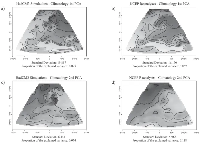
Figure 4 – Spatial PCA for the minimum extreme temperature climatology defi ned by the (a, c) HadCM3 Simulations and
the (b, d) NCEP Reanalyses.
-3*10^6 -2*10^6 -10^6 0 10^6 2*10^6 3*10^6
-2*
10
^
6
-10^
6
0
10
^
6
2*
1
0^
6
-40 -30
-30
-30
-20 -10
-10 -10
-10
-10 0
0
0 0
0
10 10
10
10 20
2020 20
30 30
-3*10^6 -2*10^6 -10^6 0 10^6 2*10^6 3*10^6
-2
*
1
0^
6
-1
0
^
6
0
1
0^
6
2
*
1
0
^
6
-40 -30
-30 -20
-20 -10
-10
-10 0
0 0
10 10
10
10
10
20
20 30
-3*10^6 -2*10^6 -10^6 0 10^6 2*10^6 3*10^6
-2
*
1
0^
6
-1
0
^
6
0
1
0^
6
2
*
1
0
^
6
-10 -10
-10 -5 -5
-5 0
0 0
00
0
5
5
5 5
5 5
5 5
5 10
10
10 10
-3*10^6 -2*10^6 -10^6 0 10^6 2*10^6 3*10^6
-2
*
1
0^
6
-1
0
^
6
0
1
0^
6
2
*
1
0
^
6
-10 -10-10
-10 -5
0
0 0
5 5
5
5 10
10
HadCM3 Simulations - Climatology 1st PCA NCEP Reanalyses - Climatology 1st PCA
a) b)
Standard Deviation: 19.857
Proportion of the explained variance: 0.895 Proportion of the explained variance: 0.867Standard Deviation: 16.170
HadCM3 Simulations - Climatology 2nd PCA NCEP Reanalyses - Climatology 2nd PCA
c) d)
Standard Deviation: 6.444
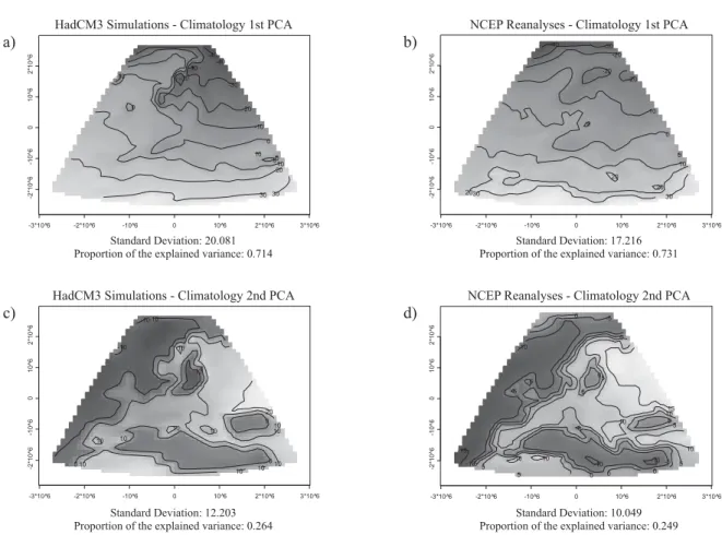
Figure 5 – Spatial PCA for the maximum extreme temperature climatology defi ned by the (a, c) HadCM3 Simulations and
the (b, d) NCEP Reanalyses.
Figure 4 and Figure 5 show the minimum and the maximum spatial PC distribution for the extremes’ mean climatology (coldest and warmest), respectively, where the spatial similarity (statistically signifi cant regions) between both models can be easily detected. Remark that in the fi gures’ label one also gives the Standard Deviation for each eigenvalue associated to each eigenvector component. Figure 6 and Figure 7 show the minimum and the maximum spatial distribution of the PC for the extremes anomaly, where a strong contrast between both models can be without diffi culty visualized; essentially with respect to the maximum system, which could be explained by model uncertainties outstanding the energy balance. There is a very high variability of the minimum extremes climatology.
The plot of the fi rst component (Figure 4) basically shows a north-south (i.e., latitudinal) gradient, and the isolines for the second component outline the European and North African land mass. The main spatial structure information can be identifi ed by the two fi rst PC’s, based upon the covariance matrix (these PCs capture most of the variance and the PC/
EOF pairs form an effi cient two-dimensional description of the fi eld). These two components, for the minimum, account about 98.9% of the total variation for the HadCM3 Simulations and 98.5% of the total variation for the NCEP Reanalyses. The highest positive loadings on the fi rst component are related to the winter’s climatology (Figure 4). This component describes the main characteristic of latitudinal, longitudinal and ocean/land variation in extreme temperatures, from the warmest environment of the south-west to the coldest of the north-east zones. The Mediterranean region and the south part of the Atlantic give high scores, while through the north and the north-east there is a preponderance of negative scores. The variable with highest positive loadings on the second component is related to the summer’s maximum climatology in opposition to the winter’s minimum climatology. This component separates contrasted warmest summer zones from coldest winter ones describing the characteristic on latitudinal variation and land/ocean balance in extreme temperature determination. The fi rst two components, for the maximum, explain about 97.8% (Figure 5) of the total variation for the
-3*10^6 -2*10^6 -10^6 0 10^6 2*10^6 3*10^6
-2
*
1
0^
6
-1
0
^
6
0
1
0^
6
2
*
1
0
^
6
-40 -40
-40
-30 -30
-20 -10
-10
0 0
00 10 10
20
3030
-3*10^6 -2*10^6 -10^6 0 10^6 2*10^6 3*10^6
-2
*
1
0^
6
-1
0
^
6
0
1
0^
6
2
*
1
0
^
6
-40 -30
-20
-20 -20
-10
0 0
0 10
20
20 20
30 30
-3*10^6 -2*10^6 -10^6 0 10^6 2*10^6 3*10^6
-2
*
1
0^
6
-1
0
^
6
0
1
0^
6
2
*
1
0
^
6
-10
-10 -10
-10
0 0
0
0
10 10 10
10 10
10
10 10
10 10 10 20
-3*10^6 -2*10^6 -10^6 0 10^6 2*10^6 3*10^6
-2
*
1
0^
6
-1
0
^
6
0
1
0^
6
2
*
1
0
^
6
-15
-10 -10
-10 -10
-5 -5
-5 -5
-5
0
0 0
0 0
0
0
0
0
5 5
5
5
5
10 10
10 10
10 15
HadCM3 Simulations - Climatology 1st PCA NCEP Reanalyses - Climatology 1st PCA
a) b)
Standard Deviation: 20.081
Proportion of the explained variance: 0.714 Proportion of the explained variance: 0.731Standard Deviation: 17.216
HadCM3 Simulations - Climatology 2nd PCA NCEP Reanalyses - Climatology 2nd PCA
c) d)
Standard Deviation: 12.203
-3*10^6 -2*10^6 -10^6 0 10^6 2*10^6 3*10^6
-2
*
1
0^
6
-1
0
^
6
0
1
0^
6
2
*
1
0
^
6
-10
-10 -10
-10 -10 -10
-10
-10
0
0
0 0
0
10 10
10 10
10 10
10
10 20
20
20
20 20
-3*10^6 -2*10^6 -10^6 0 10^6 2*10^6 3*10^6
-2
*
1
0^
6
-1
0
^
6
0
1
0^
6
2
*
1
0
^
6
-60 -40
-40
-20 -20
-20
0 0
20 20
20
20
20
20 20
40 40
40
40 40 40 60
-3*10^6 -2*10^6 -10^6 0 10^6 2*10^6 3*10^6
-2
*
1
0^
6
-1
0
^
6
0
1
0^
6
2
*
1
0
^
6 -25
-20 -20 -15-10-10 -15
-10 -10
-5
-5
-5 -5
-5
0 0
0 0
0
0 0
0
0 0
0
5
5
10
-3*10^6 -2*10^6 -10^6 0 10^6 2*10^6 3*10^6
-2
*
1
0^
6
-1
0
^
6
0
1
0^
6
2
*
1
0
^
6 -20
-10
-10 -10
-10 -10
-10 -10
0 0
0 0
0 0
0 0 0 10
10
10
10
10
HadCM3 Simulations and 98% of the total variation for the NCEP Reanalyses. The variable with highest positive loadings on the fi rst component is the winter’s minimum climatology for the HadCM3 Simulations as well as a mixed contrast between the winter’s minimum climatology and the summer’s maximum climatology for the NCEP Reanalyses (Figure 5). This component describes the main characteristic of latitudinal variation in extreme temperatures, from the warmest environment of the south to the coldest of the north zones. The variable with highest positive loadings on the second component is related to the summer’s maximum climatology in opposition to the winter’s minimum climatology. This component describes the main characteristic of latitudinal, longitudinal and ocean/land variation in extreme temperatures, from the warmest environment of the south-west to the coldest of the north-east zones;
Concerning the PCA constructed for the anomaly of long-term extreme seasonal temperature regimes, the elementary spatial structure information can be identifi ed by the fi rst two PC’s, based upon the covariance matrix (Figure 6). These two
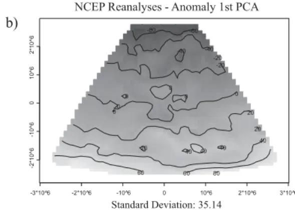
components, for the minimum, account about 95.3% of the total variation for the HadCM3 Simulations and 98.2% of the total variation for the NCEP Reanalyses. The highest positive loadings on the fi rst component are related to the winter’s climatology (Figure 6). This component describes the main characteristic of ocean/land variation in extreme temperature anomalies. The variable with highest positive loadings on the second component is related to the winter’s minimum in opposition to the summer’s maximum. This component separates contrasted largest summer anomalies from prevalent winter ones describing the characteristic on latitudinal variation and land/ocean balance in extreme temperature anomalies determination. The fi rst two components, for the maximum, explain about 89.3% of the total variation for the HadCM3 Simulations and 98.6% of the total variation for the NCEP Reanalyses (Figure 7). The variable with highest negative loadings on the fi rst component is the winter’s minimum climatology for the HadCM3 Simulations in opposition with the summer’s maximum anomaly for the NCEP Reanalyses (Figure 7). This component describes the main characteristic of latitudinal variation, mainly for the
Figure 6 – Spatial PCA for the minimum extreme temperature anomaly defi ned by the (a, c) HadCM3 Simulations and the (b, d) NCEP Reanalyses.
HadCM3 Simulations - Anomaly 1st PCA NCEP Reanalyses - Anomaly 1st PCA
a) b)
Standard Deviation: 10.275
Proportion of the explained variance: 0.674 Proportion of the explained variance: 0.908Standard Deviation: 27.519
HadCM3 Simulations - Anomaly 2nd PCA NCEP Reanalyses - Anomaly 2nd PCA
c) d)
Standard Deviation: 6.613
Figure 7 – Spatial PCA for the maximum extreme temperature anomaly defi ned by the (a, c) HadCM3 Simulations and the (b, d) NCEP Reanalyses.
NCEP Reanalyses, in extreme anomalies. The variable with highest negative loadings on the second component is related to the summer’s maximum for the HadCM3 Simulations in opposition to the summer’s maximum for the NCEP Reanalyses. This component describes the main characteristic of latitudinal, longitudinal and ocean/land variation in extreme anomalies. Based on the PCA one concludes that for extreme anomalies there is no realistic spatial agreement between the HadCM3 Simulations and the NCEP Reanalysis throughout the entire target window, local discrepancies could be explained by model uncertainties outstanding the orography, the latitudinal heat and energy balances. Although, the spatial pattern of the NCEP Reanalyses climatology is strongly recognized by the HadCM3 Simulations.
The PCA do not use external information about the phenomenon such as underlying measurements. This prior information can be extracted to quantify spatially how well the general circulation climate model reproduces the current
extreme events given by the reanalyses. Compositing all the events, reduce the number of spatial degrees of freedom by cluster (“where the system spends most of its time”) analysis, from such a region gives the corresponding spatial pattern and some additional information can be obtained by observing the spatial character of categorized events.
The naive Bayesian classifi cation or clustering is a simple probabilistic classifi cation method. The term naive Bayes refers to the fact that the probability model can be derived using Bayes’ Theorem and that it incorporates strong independence assumptions that often have no bearing in reality, hence are deliberately naive. Depending on the precise nature of the probability model, naive Bayes classifi ers can be trained very effi ciently in a supervised learning setting. Abstractly, the probability model for a classifi er is a conditional model over a dependent class variable with a small number of outcomes or classes, conditional on several feature variables through.
-3*10^6 -2*10^6 -10^6 0 10^6 2*10^6 3*10^6
-2
*
1
0^
6
-1
0
^
6
0
1
0^
6
2
*
1
0
^
6 -30-25
-20 -15
-15 -15
-15 -10
-10
-10
-10-10 -10
-10 -5
-5
-5
-5 -5
-5
-5
-5 -5 0
0 0
0 0
0
0 0
0
5
5 5
5 5
5 5
5
-3*10^6 -2*10^6 -10^6 0 10^6 2*10^6 3*10^6
-2
*
1
0^
6
-1
0
^
6
0
1
0^
6
2
*
1
0
^
6
-60 -60
-40 -40
-20 -20
0
0 0
0 0
0
20
20
20
40
40 40 40
60 60 80
-3*10^6 -2*10^6 -10^6 0 10^6 2*10^6 3*10^6
-2
*
1
0^
6
-1
0
^
6
0
1
0^
6
2
*
1
0
^
6
0 0
0 0
0
0
0
0 5
5
5
5 5
5
5
5
10 10
10
10
-3*10^6 -2*10^6 -10^6 0 10^6 2*10^6 3*10^6
-2
*
1
0^
6
-1
0
^
6
0
1
0^
6
2
*
1
0
^
6
-20
-20 -20
-20 -20
-20
-20 -20
-20 -20
-10 -10
-10 -10
-10 -10
-10 -10
0
0 0
0
0
0
0
0 10
10
10
10 10
10
10 10
10 20
20 20
20
2020
20
HadCM3 Simulations - Anomaly 1st PCA NCEP Reanalyses - Anomaly 1st PCA
a) b)
Standard Deviation: 6.516
Proportion of the explained variance: 0.673 Proportion of the explained variance: 0.876Standard Deviation: 35.14
HadCM3 Simulations - Anomaly 2nd PCA NCEP Reanalyses - Anomaly 2nd PCA
c) d)
Standard Deviation: 3.723
5. SPATIAL PATTERN BAYESIAN
CLASSIFICATION
The procedure of Bayesian Classifi cation (BC) is based on the estimation of the prior distribution upon certain global aspects of the data set (Domingos and Pazzani, 1997). It is an alternative approach to Discriminant Analysis via probability models (Ripley, 1996). The BC summarizes the evidence provided by a data set in favour of one model classifi cation, represented by a statistical model, where the prior knowledge is constructed based on the overall attribute across the spatial data (i.e., make available a measure to quantify how the HadCM3 Simulations react to a specifi c NCEP Reanalyses classifi cation). This methodology can be used for description as well as for prediction. One has developed the following exercise just to exemplify and attempt to elucidate for what kind of interpretation is expected to come out of this scheme.
Let πC = P(C) the prior spatial probabilities of the classes, assumed to have arisen under the classification according to a climate signal conditional probability function from the NCEP Reanalyses P(NCEP|C). Given the prior probabilities functions, the data C produce posterior probabilities P(C|NCEP). Since any prior information gets transformed to posterior information through consideration of the spatial ensemble C, the transformation itself represents the evidence provided by C. In fact, the same transformation is used to obtain the posterior probability, regardless of the prior probability and this transformation takes a simple form, from the Bayes’ theorem (Kass and Raftery, 1995; Carlin and Louis, 2002).
In practice consider the Boolean classification problem concerning the multinomial climate signal domain presupposing the stochastic function {Z(s), s ∈ ℜ2} taking values 1, 2, 3 or 4. Consequently, the HadCM3 Simulations can be represented by a realization of {Z(s), s ∈ ℜ2} given by {z(si), i = 1, ..., n} Z = 1, 2, 3, 4, by means of
the inter-quartile subdivision of the NCEP Reanalyses πC
j = P(Cj(s)), ∀j = 1,2,3,4 representing the spatial
target-classifier (Figure 8). According to the Bayes’ theorem, the probability of the {Z(s)} = {z(si), i = 1, ..., n} being
class Cj is:
P C s z s P z s z s C P z s z s
j
n j
n
C
( ) ( ) , ..., , ...,
(
)
=(
{
( )
( )
}
)
( )
( )
{
}
(
)
⋅1
1
π jj, ∀ =j 1 2 3 4, , ,
(1) The probability ratios also called discriminant functions can be expressed in terms of a series of likelihood ratios:
P C s z s z s
P C s z s z s
j n
k n
k j
( ) ,...,
( ) ,..., , ,
1
1
1 2
( )
( )
{
}
(
)
( )
( )
{
}
(
)
≠ = 33 41
1
,
,..., | ( ) ,..., | ( )
=
( )
( )
{
}
(
)
( )
( )
{
}
(
)
⋅P z s z s C s P z s z s C s
n j
n k
π π
π
C
C k j
j
k
≠ =1 2 3 4, , ,
(2)
The probabilities on the prediction are crucial for optimal decision making. The cost of predicting for z(si) class Ck when
the true class is Cj, k ≠ j, is designated by χ(k, j, z). The Bayes
optimal prediction for z(si) is the class Ck that minimizes the
expected loss (i.e., the expected cost of predicting z(si) belongs
to a given class Ck):
ℓ k z s P C z s k j z
i j i
j
| ( ) | ( ) ( , , )
(
)
=∑
(
)
⋅χ (3)In fact, one is interested on the spatial true rate of a classifi er; it means the empirical frequency of locations correctly classifi ed. In real life, this naive Bayes approach is more powerful than might be expected from the extreme simplicity of its model; in particular, it is fairly robust in the presence of non-independent attributes (Zhang et al. 2000). Recent theoretical analysis has shown why the naive Bayes classifi er is so robust (Rish et al. 2001).
There is a slight visual inconsistency between the HadCM3 Simulations (isotherms) and the NCEP Reanalyses inter-quartile classifi cation of extreme temperature climatology over the target domain. This unpredictability can be established by the reciprocal classifi cation. The HadCM3 Simulations produce unrealistically extreme temperature events for the winter ensemble with misclassifi cation of about 5% and a signifi cant divergence regarding the summer of about 25%, there is a signifi cant divergence regarding the summer time as well, the misfi t is about 25% (Figure 8 and Figure 9).
Model Calibration by Relative Risk Assessment: The
-3*10^6 -2*10^6 -10^6 0 10^6 2*10^6 3*10^6 -2 * 1 0^ 6 -1 0 ^ 6 0 1 0^ 6 2 * 1 0 ^ 6
1 1 1 12 2 2 2 2 2 1 1 1 11 1 1 1 12 2 2 2 2 2 2 2 2 1 11 1 1 2 22 2 3 3 3 2 2 1 1 11 11 2 3
3 3 3 3 3 3 1 1 1 1 1 11 1 1 3
3 3 3 33 3 1 1 1 11 11 1 3 33333 11121111 11 344 43 3 11 1 2 21 1 111 4
4 4 2 4 3 3 3 1 3 2 1 1 1 1 1 4 4
4 2 4 3 3 2 3 3 1 1 1 1 1 1 4
4 2 2 3 3 2 2 2 1 1 1 1 1 1 1 4
4 4 4 2 2 2 2 2 1 1 1 1 1 1 1 4 4
4 4 2 3 2 1 2 2 1 1 1 1 1 1 4
4
4 4 2 2 1 2 2 2 2 1 3 3 3 1 4
4
3 3 2 4 4 2 4 1 2 2 3 3 3 2 4
4 3
3 2 4 4 4 4 4 2 2 2 2 1 1 4
4 3
3 4 4 4 4 4 4 4 4 2 2 2 2 4
4 4
3 3 3 3 4 4 4 4 4 4 4 2 2 4
4
3 3 2 3 3 3 4 4 4 4 4 4 2 3 4
4
3 3 3 3 3 3 3 3 3 3 3 3 2 2 -40 -30 -30 -30 -20 -20 -20 -10 -10 -10 -10 -10 -10 0 0 0 0 0
10 10 10
-3*10^6 -2*10^6 -10^6 0 10^6 2*10^6 3*10^6
-2 * 1 0^ 6 -1 0 ^ 6 0 1 0^ 6 2 * 1 0 ^ 6
1 1 1 11 1 2 2 2 1 1 1 1 11 1 1 1 11 2 2 2 2 2 2 2 1 1 11 1 1 1 22 2 2 2 2 2 2 1 1 11 11 2 2
2 2 2 2 2 2 1 1 1 1 1 11 1 1 3
3 3 3 32 2 1 1 1 11 11 1 3 33333 11121111 11 3 33 33 31 1 1 2 21 1 111 3 3
3 2 3 3 3 2 1 2 2 1 1 1 1 1 3 3 3 2 3 3 3 2 2 2 1 1 1 1 1 1 4
4 2 2 2 3 2 2 2 1 1 1 1 1 1 1 4 4
3 3 2 2 2 2 2 1 1 1 1 1 1 1 4
4
4 3 2 3 2 1 2 2 2 1 1 1 1 1 4
4 4 4
2 2 2 2 2 2 2 1 2 2 2 1 4
4 3 3 3 4 3 2 3 1 2 2 3 3 3 2 4
4
3 3 3 4 4 3 4 3 2 2 2 2 2 2 4
4
3 3 4 4 4 4 4 4 4 3 2 2 3 2 4
4
4 3 3 3 3 4 4 4 4 4 4 4 3 3 4
4
3 3 3 3 4 4 4 4 4 4 4 4 3 3 4
4
3 4 4 4 4 4 4 4 4 4 4 4 4 4 -30 -20 -20 -10 -10 0 0 0 10 10
-3*10^6 -2*10^6 -10^6 0 10^6 2*10^6 3*10^6
-2 * 1 0^ 6 -1 0 ^ 6 0 1 0^ 6 2 * 1 0 ^ 6
1 1 1 11 1 1 1 1 1 1 1 1 11 1 1 1 11 1 1 1 1 1 1 1 1 1 11 1 1 1 11 1 1 1 1 1 1 1 1 11 11 1 1
1 1 1 1 1 1 1 1 1 1 1 11 1 1 1
1 1 1 11 1 1 1 1 22 2 2 2 1 11111 11112222 22 111 11 1 11 2 1 12 2 222 11 2 1 1 1 1 1 2 1 1 3 2 2 2 2 1
1 2 2 2 2 2 2 1 1 3 3 2 3 3 3 1 2
2 2 2 2 3 3 3 3 3 3 3 3 3 3 2
2 2 2 2 2 2 2 2 2 3 3 3 3 3 3 2
2 2 2 3 3 2 1 2 3 3 2 3 4 4 4 2
2
2 3 3 2 2 2 2 3 3 3 2 3 3 3 2
3
2 2 2 3 4 3 4 2 2 3 3 3 3 2 3
3
3 2 3 4 4 3 4 4 3 4 2 2 1 1 3
3
4 3 3 4 4 4 4 4 4 4 2 2 2 3 3
4 4
4 4 4 4 4 4 4 4 4 4 4 4 4 4
4 4
3 4 4 4 4 4 4 4 4 4 3 3 4 4
4 4
4 4 4 4 4 4 4 4 4 4 3 3 4 5 10 15 15 20 20 20 20 25 25 25 25 25 25 25
-3*10^6 -2*10^6 -10^6 0 10^6 2*10^6 3*10^6
-2 * 1 0^ 6 -1 0 ^ 6 0 1 0^ 6 2 * 1 0 ^ 6
1 1 1 11 1 1 1 1 1 1 1 1 11 1 1 1 11 1 1 1 1 1 1 1 1 1 11 1 1 1 11 1 1 1 1 1 1 2 2 21 11 1 1
1 1 1 1 1 1 2 2 2 2 2 22 1 1 1
1 1 1 11 1 2 2 1 22 2 2 2 1 1111122 212322 32 11 11 11 2 2 2 1 13 33 33 1 1 1 2 1 1 1 1 2 1 1 3 3 3 3 3 1
1 1 2 1 1 1 3 1 1 3 3 3 3 3 4 1 1 2 2 2 1 3 3 3 3 3 3 4 4 4 4 1
1 1 1 3 3 3 3 3 3 3 3 4 4 4 4 1
1 1 2 3 3 3 2 3 4 3 4 4 4 4 4 1
1
2 2 4 3 3 4 3 4 4 4 2 2 2 4 2
2
4 4 3 2 2 4 2 4 3 4 2 2 2 4 2
2
4 4 4 2 2 2 2 2 4 4 3 4 3 4 2
2
4 4 2 2 3 2 2 2 3 2 4 4 4 4 2
2 2
4 4 4 4 3 2 2 2 3 3 2 4 4 2
2 4
4 4 4 4 4 3 3 2 2 2 2 4 4 2
2 4
4 4 4 4 4 4 4 4 4 4 4 4 4 10 20 20 20 30 30 30 30 40 40 40 40 40 50
5050 50 -3*10^6 -2*10^6 -10^6 0 10^6 2*10^6 3*10^6
-2 * 1 0^ 6 -1 0 ^ 6 0 1 0^ 6 2 * 1 0 ^ 6
1111111122222222211111111111111 1111111122222222222222222222222 1111122222223333322222222222222 1222222223333333222111111222222 2222333333333332111111111111111 2233333333333322111111111111111 2333333 33 3333211111111111111111 33 3 3
3 3 3 3 33 33 1 1 1 1 1 1 2 2 1 1 11 1 11 111 1 4 4 44 3 3 3 3 3
3 3 2 1 1 1 1 1 2 2 2 2 1 1 11 1 11 1 1 1 4 4 4 43 3 3 3 3 3
3 3 3 2 2 2 2 2 3 2 2 2 11 1 11 1 11 1 4 4 4
4 3 3 3 33 4 3 3 3 3 3 2 2 3 3 2 1 1 1 11 1 11 1 1 1 4 4 4
4 3 3 3 33 3 3 3 3 2 2 2 2 2 2 2 1 1 1 11 1 11 1 1 1 4 4 4
3 3 3 33 3 3 3 2 2 2 2 2 2 1 1 1 1 1 1 11 1 11 1 1 1 4 4 4
4 4 4 33 3 2 2 2 2 2 2 1 1 1 1 1 1 1 1 11 1 11 1 1 1 4 4 4
4 4 4 4
3 2 2 2 2 2 1 1 1 1 1 1 1 1 1 1 11 1 11 1 1 1 4 4 44 4 4
4 3 2 2 2 2 1 1 1 1 1 1 2 1 1 1 1 1 22 22 2 1 1 4 4 44 4 4
4 3 2 2 2 2 2 22 3 2 2 2 1 1 12 2 3 3 33 3
2 1 4 4 4
4 3 3 3
2 2 2 3 4 4 4 3 3 3 3 2 2 1 2 2 33 33 3 3 32 4 44 4 3
2 2 2 3 44 4 4 4 4 4 3 4 3 2 2 2 22 22 22 2 2 1 4 44 4 3
2 2 3 4 44 4 4 4 4 4 4 4 4 3 3 3 32 21 11 1 1 1 4 44 4 4
3 3 3 44 4 4 4 4 4 4 4 4 4 4 3 4 43 2 22 2 2 22 4 4
4 4 4
3 4 4 3 33 3 3 3 4 4 4 4 4 4 4 4 44 4 44 4 2 22 4 4
4 4 3
2 2 3 2 22 3 3 3 3 4 4 4 4 4 4 4 44 4 44 3 2 22 4 4
4 4 3
2 2 3 32 3 3 3 3 3 3 3 4 4 4 3 3 44 44 43 2 2 2 4 4
4 3 2
2 3 3 332 3 3 3 2 2 3 3 3 3 3 33 3 33 3 3 22 2 -40 -40 -40 -20 -20 -20 -20 0
0 0 0
-3*10^6 -2*10^6 -10^6 0 10^6 2*10^6 3*10^6
-2 * 1 0^ 6 -1 0 ^ 6 0 1 0^ 6 2 * 1 0 ^ 6
1111111111122221111111111111111 1111111111222222222222222221111 1111111222222222222222222222222 1112222222222222221111111111222 2222222222333222111111111111111 2222222223333221111111111111111 2222333 33 33322 1 11 1 11 1 111 111111 1 33 3 3
3 3 3 3 33 32 1 1 1 1 1 1 1 1 1 1 11 1 11 111 1 3 3 33 3 3 3 3 3
3 2 2 1 1 1 1 1 2 2 2 1 1 1 11 1 11 1 1 1 3 3 3 33 3 3 3 3 3
3 3 2 2 2 2 2 2 2 2 2 1 11 1 11 1 11 1 3 3 3
3 3 3 3 33 3 3 3 3 2 2 2 2 2 2 2 1 1 1 11 1 11 1 1 1 3 3 3
3 3 3 3 33 3 3 3 2 2 2 2 2 2 2 1 1 1 1 11 1 11 1 1 1 3 3 33 3 3 3
3 3 3 3 2 2 2 2 2 2 2 1 1 1 1 1 11 1 11 1 1 1 3 3 3
3 3 3 33 3 2 2 2 2 2 2 2 2 1 1 1 1 1 1 11 1 11 1 1 1 4 4 4
3 3 3 33 2 2 2 2 2 2 1 1 1 1 1 1 1 1 1 11 1 11 1 1 1 4 4 44 4 4
3 3 2 2 2 2 2 2 22 2 2 2 2 2 11 1 1 1 11 2
1 1 4 4 4
4 3 3 3
3 2 2 2 2 2 2 2 2 2 2 2 2 1 1 2 22 22 2 2 21 4 44 4 3
3 3 2 23 3 3 3 3 3 3 3 3 2 2 1 2 22 3 33 3 3 22 4 44 4 3
3 2 2 33 4 4 4 4 4 3 3 3 3 2 2 2 22 22 22 2 2 2 4 4
4 4 3
3 3 3 3 44 4 4 4 4 4 4 4 3 3 3 3 32 22 22 2 2 2 4 4
4 4 44 3 3 4
4 4 4 4 4 4 4 4 4 4 3 3 3 33 3 32 2 2 22 4 4
4 4 4
4 3 3 3 33 3 4 4 4 4 4 4 4 4 4 44 4 44 4 3 33 3 4 4
4 4 4
3 3 3 3 34 4 4 4 4 4 4 4 4 4 4 4 44 4 44 4 3 34 4 4
4 4 4
3 3 4 44 4 4 4 4 4 4 4 4 4 4 4 4 44 44 44 3 3 4 4 4
4 4 4
4 4 4 444 4 4 4 4 4 4 4 4 4 4 44 4 44 4 4 44 4 -50 -40 -40 -40 -40 -40 -30 -30 -30 -20 -20 -10 -10 -10-10 0 0 10 10 10 10
-3*10^6 -2*10^6 -10^6 0 10^6 2*10^6 3*10^6
-2 * 1 0^ 6 -1 0 ^ 6 0 1 0^ 6 2 * 1 0 ^ 6 1111111111111111111111111111 1111111111111111111111111111111 1111111111111111111111111111111 1111111111111111111111111111111 1111111111111111111111111111111 11111
11111111111111111222221112 1111111 11 1111111111112222222222 11 1 1
1 1 1 1 11 11 1 1 1 1 1 1 1 2 2 2 22 2 22 222 2 1 1 1
1 1 1 1 1 11 1 1 1 1 1 1 1 2 2 2 2 2 2 22 2 22 22 2 1 1 1 1
1 1 1 1 1 11 1 1 2 2 2 2 2 2 2 2 2 22 3 32 2 22 2 1 1 1
1 1 1 1 11 1 2 2 2 3 2 3 2 2 2 2 2 2 2 22 2 22 23 3 1 1 11 1 1 1 1
1 2 2 2 2 3 3 3 2 3 3 3 3 2 2 22 2 22 2 3 3 1 1 12 2 1 2
2 2 2 2 2 2 2 3 3 3 3 3 3 2 2 2 33 3 33 3 3 3 2 2 2
2 2 2 22 2 2 3 3 3 2 2 2 2 2 2 2 2 2 2 33 3 33 3 3 3 2 2 22 2 2 2
2 2 2 3 2 2 1 1 2 2 2 2 2 2 2 2 23 3 33 3 3 3 2 2 22 2 3
3 3 3 3 2 2 1 1 1 1 2 2 3 3 2 2 2 3 33 33 43 3 3 3 32 2 3
3 3 3 3 3 2 2 22 3 3 3 3 2 2 23 3 4 4 44 43 3 3 3 3
3 2 2 33 3 3 3 3 3 4 3 3 4 3 3 2 2 2 3 44 33 44 3 2 3 33 3 3
2 2 2 3 44 4 4 4 4 4 3 4 3 3 2 3 33 32 22 22 1 3 33 3 3
3 3 3 4 44 4 4 4 4 4 4 4 4 3 3 4 43 22 12 22 2 3 33 3 4
3 3 4 44 4 4 4 4 4 4 4 4 4 4 4 4 44 3 33 3 3 34 3 33 4 4
4 3 3 4 44 4 4 4 4 4 4 4 4 4 4 4 44 4 44 4 4 44 3 33 4 4
4 4 4 4 44 4 4 4 4 4 4 4 4 4 4 4 44 4 44 3 3 44 3 33 4 4
4 4 4 44 4 4 4 4 4 4 4 4 4 4 4 3 34 44 4 3 34 4 3 33 4 4
4 4 4 444 4 4 4 4 4 4 4 4 4 4 43 3 33 3 3 34 4 5 5 10 10 15 15 15 20
20 20 20
20 25
25
25 30
-3*10^6 -2*10^6 -10^6 0 10^6 2*10^6 3*10^6
-2 * 1 0^ 6 -1 0 ^ 6 0 1 0^ 6 2 * 1 0 ^ 6 111111111111111111111111 111 1111111111111111111111111111111 1111111111111111111111111111111 1111111111111111111222222211111 1111111111111111212222222222221 11111
11111111112222222222221112 1111
111 11 11111 2 22 2 21 1 333 322222 2 11 1 11 1 1 1 11 1
1 1 2 2 2 2 2 1 1 3 3 33 3 33 33 3 2 1 1 1
1 1 1 1 1 11 1 2 2 2 2 2 2 2 1 1 1 3 3 33 3 33 33 2 1 1 1 11 1 2 1 1 1
1 1 1 1 1 3 3 1 1 1 1 3 33 3 33 3 3 3 3 1 1 11 1 2 2 1
1 1 1 1 1 3 2 3 3 2 2 2 3 3 3 33 3 33 3 3 3 1 1 1
1 2 1 1 21 1 1 1 2 3 3 3 2 3 3 3 3 3 3 33 3 33 3 3 3 1 1 1
2 2 1 22 2 1 1 3 3 3 3 3 3 3 3 3 3 3 3 33 3 33 3 3 3 1 1 1
1 1 1 11 2 3 3 3 3 3 3 3 3 3 3 3 3 3 3 33 3 33 3 3 4 1 1 1
1 1 1 13 3 3 3 3 3 2 2 2 2 3 3 3 3 3 3 33 4 44 4 4 4 1 1 11 1 1
2 2 4 4 3 3 3 2 22 3 3 3 3 3 33 3 44 4 4 24 4 1 1 1
1 1 2 22 4 4 4 3 3 3 3 2 4 4 4 4 4 3 3 42 22 22 4 4 1 12 2 4
4 4 4 44 2 2 2 2 4 4 2 2 4 4 4 4 42 2 22 2 2 23 2 22 2 4
4 4 4 42 2 2 2 2 2 2 4 2 2 4 4 4 44 44 34 44 3 2 22 2 4
4 4 4 2 22 2 2 2 2 2 2 2 3 4 4 3 34 44 44 44 4 2 22 2 4
4 4 4 32 2 2 2 2 2 2 2 2 2 3 4 3 34 4 44 4 4 44 2 2
2 2 3
4 3 3 4 44 4 4 4 3 3 2 2 2 2 2 22 2 23 3 3 44 4 2 22 2 4
4 4 4 4 44 4 4 4 4 3 3 2 2 2 2 2 22 2 22 4 4 44 2 2
2 4 4
4 4 4 44 4 4 4 4 4 4 4 3 3 4 4 4 43 22 24 4 4 4 2 2
2 4 4
4 4 4 444 4 4 4 4 4 4 4 4 4 4 44 4 44 4 4 44 4 10 10 10 20 20 30 30 40 40 40 40 40 40 40 40 50
Figure 8 – Spatial Interquartile (IQ thresholds) climate signal by the NCEP Reanalyses classifi cation with the
interpolated isotherms from the HadCM3 Simulations (a) minimum, (b) maximum.
HadCM3 Climatology by NCEP IQ Climate Signal - TMIN.W a)
IQ: (-42.86, -20.61, -7.37, 1.02, 14.84) °C IQ: (-35.13, -10.13, -0.50, 8.13, 16.35) °C
HadCM3 Climatology by NCEP IQ Climate Signal - TMAX.S b)
IQ: (1.36, 16.12, 18.90, 23.22, 30.18) °C IQ: (2.76, 21.34, 28.98, 34.24, 53.32) °C
NCEP Climatology by HadCM3 IQ Climate Signal - TMIN.W a)
IQ: (-55.68, -21.83, -7.72, 1.23, 16.45) °C IQ: (-50.74, -13.82, -2.21, 6.69, 17.35) °C
NCEP Climatology by HadCM3 IQ Climate Signal - TMAX.S b)
IQ: (2.02, 14.85, 19.12, 22.48, 30.43) °C IQ: (2.82, 18.98, 26.71, 34.11, 51.04) °C
Figure 9 – Spatial Interquartile (IQ thresholds) climate signal by the HadCM3 Simulations classifi cation with the
-3*10^6 -2*10^6 -10^6 0 10^6 2*10^6 3*10^6
-2
*
1
0^
6
-1
0
^
6
0
1
0^
6
2
*
1
0
^
6
-2
-2 -2
-2 -2
-2 -2
-2
-2 -1-1
-1
-1 -1
-1
-1 -1
-1 0
0 0
0
0 0
0 0
0
0 0
0 0 0 0
0
-3*10^6 -2*10^6 -10^6 0 10^6 2*10^6 3*10^6
-2
*
1
0^
6
-1
0
^
6
0
1
0^
6
2
*
1
0
^
6
-2
-2 -2
-2
-2 -2 -1
-1
-1 -1 -1
-1 -1
0
0 0
0 0
0
0 0
0 0
-3*10^6 -2*10^6 -10^6 0 10^6 2*10^6 3*10^6
-2
*
1
0^
6
-1
0
^
6
0
1
0^
6
2
*
1
0
^
6
-2-2 -2 -2
-1
-1
-1 -1
-1
-1
-1 0
0 0
0
0 0
0 0
0 0
0
0
-3*10^6 -2*10^6 -10^6 0 10^6 2*10^6 3*10^6
-2
*
1
0^
6
-1
0
^
6
0
1
0^
6
2
*
1
0
^
6
-2 -2
-2
-2
-2 -2
-2 -2
-1 -1
-1
-1 -1
-1
-1
0
0
00 0
0
0 0
0 0
0 0
0 0 0
0 0
0 0
0 0 0
0
6. SUMMARY
This manuscript is an attempt to compare patterns of extreme temperature anomalies simulated by the GCM (HadCM3) with NCEP/NCAR Reanalyses over a sector in Europe. The spatial patterns of extreme anomalies in the NCEP Reanalyses are not recognized from the HadCM3 model. Such instability may persist in the future. In all variables the same spatial climatology pattern is detected, suggesting that the ensemble describes the main characteristic of spatial variation in temperature extremes, from the temperate climates of the southwest zones to the extreme cold of the northeast ones. The HadCM3 Simulations are not able to fi t reasonably the regimes defi ned by the NCEP Reanalyses. This is evidenced by the analyses carried out in this paper.
The procedures described here are useful for two reasons. First, they help to prevent model misspecifi cation, which can lead to incorrect conclusions regarding accuracy and effi cacy. Second, they provide information about the relationship between prognostic factors (predictive location-based) and extreme risk. As a matter of fact, all diagnostic based on PCA and BC reject the hypothesis that the HadCM3 Simulations are adequate for modeling present-days scenarios of extremes based on the NCEP Reanalyses. Nevertheless, the HadCM3 Simulations fi t quite well the spatial climate
regimes defined by the NCEP Reanalyses. Climatic risk analyses and forecasting, concern among others topics, assess and interpretation changes in the intensity and frequency of recurrence of long duration extreme values (heat/cold waves). So, information and incorporation of other extreme indices into the analysis are strongly advisable.
Though uncertainties are inherent in any statistical model, they can be reduced by judicious choices of other methods. In the context of the extreme value analysis, possibilities include the use of alternative models that confi rm the information obtained in this exploratory analysis. Additionally, only the prognostic factors (predictive location-based) and not the extreme hazard (vulnerability severe-extreme-based) were considered in this study. The objective of this basic analysis was just to present a way to assess spatial extremes of a particular GCM, analyzing the uncertainty introduced by the inability of HadCM3 Simulations to adequately reproduce the current climate by statistical modeling.
PCA and BC are very powerful tools to model extreme hazards and future uncertainties by means of location-based prediction. It is an alternative method to capture local suspicions of lack of information. This exploratory work is essential, as it identifi es the strengths and weaknesses of GCM to regional-scale differences in model performance, providing insights on regional-scale climate interactions and processes.
Figure 10 – The spatial Relative Risk via Discriminant Analysis of the Bayesian Classifi cation based on the NCEP
Reanalyses IQ climate signal (a) minimum, (b) maximum designed for the HadCM3 Simulations.
Expected Cost of Predicting HadCM3 from NCEP Classifi er - TMIN.W a)
7. ACKNOWLEDGMENTS
This work is an autonomous contribution to the EU funded MICEproject (Modelling the Impacts of Climate Extremes: MICE EVK2-CT-2001-00118). Model data were supplied by the Climate Impacts LINK project (funded by the UK Department of the Environment, Food and Rural Affairs) on behalf of the Hadley Centre for Climate Prediction and Research, which is part of the Met Offi ce in the UK (the National Meteorological Service). The fi nancial supports of FCT (Portugal) and ICAT-FCUL (Portugal) are also acknowledged. Appreciative thanks to the referees and the journal editor; their comments were very useful in improving this paper.
8. REFERENCES
BAILEY, T. C.; GATREL, A. Interactive Spatial Data
Analysis. Prentice Hall, 1996. 413p.
de BOOR, C. A Practical Guide to Splines. Reprint edition,
Springer, 1994. 416p.
CARLIN, B. P; LOUIS, T. A. Bayes and Empirical Bayes
Methods for Data Analysis. 2nd edition, Chapman and
Hall/CRC, 2002. 440p.
CRESSIE, N. A. C., Change of support and the modifi able area unit problem. Geographical Systems, v. 3, p.
159-180, 1996.
DOMINGOS, P.; PAZZANI, M. Beyond independence: Conditions of the optimality of the simple Bayesian classifi er. Machine Learning, v. 29, p. 103-130, 1997.
DRAPER, N. R.; SMITH, H. Applied Regression Analysis.
3rd edition, Wiley-Interscience, 1998. 736p.
FUENTES, M.; GUTTORP, P.; CHALLENOR, P. Statistical Assessment of Numerical Models. NRCSE Technical
Report Series 076, University of Washington Press, 2003.
GORDON, C.; COOPER, C.; SENIOR, C. A.. BANKS, H.. GREGORY, J. M.. JOHNS, T. C.; MITCHELL, J. F. B.; WOOD, R. A. The simulation of SST, sea ice extents and ocean heat transports in a version of the Hadley Centre coupled model without fl ux adjustments. Climate
Dynamics, v. 16, p. 147-168, 2000.
JOHNSON, R. A.; WICHERN, D.W. Applied Multivariate
Statistical Analysis. 4th edition, Prentice Hall, 1998. 799p.
KALNAY, E.; KANAMITSU, M.; KISTLER, R.; COLLINS, W.; DEAVEN, D.; GANDIN, L.; IREDELL, M.; SAHA, S.; WHITE, G.; WOOLLEN, J.; ZHU, Y.; CHELLIAH, M.; EBISUZAKI, W.; HIGGINS, W.; JANOWIAK, J.; MO, K. C.; ROPELEWSKI, C.; WANG, J.; LEETMAA, A.; REYNOLDS, R.; JENNE, R.; JOSEPH, D. The NCEP/ NCAR 40-year reanalysis project. Bull. Am. Meteorol. Soc.,
v. 77, p. 437-471, 1996.
KASS, R.; RAFTERY, A. Bayes factors and model uncertainty.
J. Amer. Statist. Assoc., v. 90, p. 773-795, 1995.
KIM, K.-Y.; NORTH, G. R. EOF analysis of surface
temperature fi eld in a stochastic climate model. J. Climate,
v. 6, p. 1681-1690, 1993.
KYSELY, J. Comparison of extremes in GCM-simulated, downscaled and observed central-European temperature series. Climate Research, v. 20, p. 211–222, 2002a.
KYSELY, J. Probability estimates of extreme temperature events: Stochastic modelling approach vs. extreme value distributions. Studia Geophysica et Geodaetica, v. 46, p.
93–112, 2002b.
LUCIO, P. S., Geostatistical assessment of HadCM3 simulations via NCEP reanalyses over Europe. Atmospheric Science
Letters, v. 5, p. 118-133, 2004a.
LUCIO, P. S. Assessing HadCM3 simulations from NCEP reanalyses over Europe: Diagnostics of block-seasonal extreme temperature’s regimes. Global and Planetary
Change, v. 44, p. 39-57, 2004b.
MATHSOFT, 2000. S-Plus 2000. Guide to Statistics. Data Analysis Products Division, MathSoft: Seattle.
MORAN, P. A. P. The interpretation of statistical maps. Journal
of the Royal Statistical Society, Series B, v. 10, p.
243-251, 1948.
NORTH, G. R.; BELL, T. L.; CAHALAN, R. F.; MOENG, F. J. Sampling errors in the estimation of empirical orthogonal functions. Mon. Wea. Rev., v. 110, p. 699-706, 1982.
POPE, V. D.; GALLANI, M. L.; ROWNTREE, P. R.; STRATTON, R. A. The impact of new physical parametrizations in the Hadley Centre climate model - HadAM3. Climate Dynamics, v. 16, p. 123-146,
RIPLEY, B. D. Pattern Recognition and Neural Networks.
Cambridge University Press, 1996. 415p.
RISH, I.; HELLERSTEIN, J.; JAYRAM, T. An analysis of data characteristics that affect naive Bayes performance. IBM T. J. Watson Research Center, Technical Report RC
21993, 2001.
von STORCH, H. On the use of “inflation” in statistical downscaling. Journal of Climate, 12, p. 3505-3506, 1999.
ZHANG, H.; LING, C. X.; ZHAO, Z. The learnability of naive Bayes. Lecture Notes in Computer Science, v. 1822, p.