Agent-based distributed time series forecasting system
Michał Zabłocki1
1
Faculty of Computer Science and Information Technology, West Pomeranian University of Technology, Szczecin, Poland
Abstract: Many studies have demonstrated that agent-based distributed computing improves quality of distributed computations. In this paper, self-aware software agents are used to manage the distributed computations in order to improve effectiveness of investment decisions. A distributed time series forecasting approach based on the modified Group Method Data Handling (GMDH) method and agent oriented programing is proposed. The forecasted re-sults computed by agents are used to make an investment decision. To assess the effective-ness of the system, we used the time series of EUR/USD currency pair stock prices. The em-pirical results with a real data set clearly suggest that the system can be deployed on the trading platform to automate process of the prediction of financial markets.
Keywords: time series prediction, GMDH, stock market forecasting, multiagent system, distributed system
1. Introduction
The current theory of economic forecasting is based almost only on the theory of probability and mathematical statistics. However, practice shows that this is not enough. Nowadays, it is believed that only use of sophisticated methods of modern technical analysis (using artificial neural networks, pattern recognition, genetic algorithms, etc.) makes sense during creation of complex models in order to reproduce the economic reality. Many Nobel Prize winners in Economics of last few years, despite the deliberately made mistakes (at simplifying the assumptions necessary to build the model), contributed to the significant knowledge increase about mathematical modeling.
Wiliński [1] used GMDH (Group Method of Data Handling) [2] as an effective methods of forecasting economic time series. A basis for GMDH by the first time was proposed in [3][4][5][6][7] by Ivakhnenko. The method, in the part related to the forecasting model, is based on two principles:
• to build the best regression model, and
• to reduce the complexity of the regression model to the lowest level acceptable by a
researcher.
best models, instead of the best single model, in order to leave a freedom in decision-making at next step.
Combinatorial Algorithm is the basic GMDH algorithm. In its original idea it was proposed by prof. Ivakhnenko. In the most general form of the algorithm is composed of multiple layers of active neurons, which resembles a neural network. The purpose of each layer is a selection of outputs from the previous layer and building a model based on external criteria. At each stage (the output of each layer), such model can be used for forecasting.
Neuron activity is based on the selection of the internal standard pool of inputs (from the previous layer) to build its model meets the external criterion and can be used as input for the next layer.
A set of models obtained by the use of GMDH can be broadly defined as a subset of Gabor-Kolmogorov polynomial.
y=α0+
∑
i=1
M
αixi+
∑
i=1M
∑
j=1
M
αijxixj+
∑
i=1M
∑
j=1
M
∑
k=1
M
αijkxixjxk+... (1)
where: α0 – constant term of a polynomial, Α(αi, αij, αijk, ...) – vector of coefficients, Χ(xi,
xj, xk, ...) – vector of variables.
Combinatorial algorithm is relatively simple linear variation of the method, but in many cases very effective. The simplicity of the algorithm is seeming, as with the growth of variable numbers, the computational complexity increases rapidly and it is necessary to impose restrictions that result from the limited time and computational power. For this reason, it becomes necessary to create subsets of models, instead of searching all possible solutions.
The GMDH, due to the fact that it requires several complex tasks to be performed (the construction, evaluation and selection of many regression models), in many cases requires huge computational power. This demand, in spite of the enormous technological progress in the field of computer technology, may not always be met by a single computer. In many cases, the forecasts that we want to build have a small horizon. So, for obvious reasons, the calculation time can not transcend that horizon. The solution to this problem may be scattering calculations on several computers.
The proposed time series forecasting system is based on distributed agent-based solution. Namely, a few software agents cooperate with each other in order to compute the forecast. Such multiagent system gains new capabilities that gives agent-oriented programming (AOP) paradigm [8].
2. Related works
Nowadays, the GMDH algorithms are widely used and many modifications of them are still developed by many researchers. Below are presented quite new and most interesting applications of this model computation technique.
In [9] authors compare the accuracy of GMDH Analogues Complexing as typical non-parametric method and the Group of Adaptive Models Evolution (GAME, also based on GMDH theory) as a parametric method. They use medical data from Motol hospital in Pra-gue and horticulture data from Hort Research New Zealand. The results of their experiments showed that both methods have good performance.
study the application of GLSSVM for monthly river flow forecasting of Selangor and Bar-man River. The results point that the proposed solution is a strong tool to build model of time series that is accurate enough to be applied successfully in prediction task.
In [11] a updated GMDH algorithm is used for medical image recognition. It is applied to medical image analysis of cancer of the liver. In this paper authors propose a novel feed-back loop application in GMDH algorithm. In this approach, to organize the neural network architecture, a two types of neurons are applied: the polynomial type and the radial basis function (RBF)-type. It is shown that the feedback GMDH-type neural network algorithm is an accurate and a useful method for the nonlinear system identification.
In this paper [12] GMDH (Group Method of Data Handling) has been applied for the identification of a mathematical model with many input variables. Proposed a Neuro-fuzzy GMDH model, adopting Gaussian radial basis functions (GRBF) as both a simplified fuzzy reasoning model and as a three-layered neural network. The Neuro-fuzzy GMDH algorithm is used for prediction of air pollution data. The authors compared the prediction accuracy of Neuro-fuzzy GMDH and Multi-Layer Perceptron (MLP).
3. Description of the algorithm
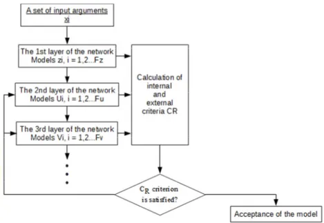
Figure 1 shows the most general scheme of the algorithm, which illustrates how to achieve a sufficient complexity of the model. Algorithm receives a set of input variables (hereinafter referred to as arguments). In the first layer the selection of the arguments is made. The selected arguments should allow to build a model that will meet internal or ex-ternal criterion. Inex-ternal criterion allows the constructed model to pass to the next layer, whereas the external criterion defines the requirements for the final model that is suitable for forecasting. Both of these criteria are selected in the learning process.
Figure 1. Overall scheme of combinatorial algorithm, source [1], p. 41
Wiliński [1] has modified combinatorial algorithm and divided it into two algorithms. These algorithms have different objectives and with varying degrees they use historical data. The first algorithm, in the first layer, for each pair of arguments, calculates a linear re-gression model:
̂
Variables xi and xj are the time series of explanatory variables X, where i and j are the
num-bers of these series, but i ≠ j. Those time series have the same length but different time shifts regarding to the current moment. Neurons of the first layer examine the pairs of arguments by selection of the numerical coefficients vector Aij = [a0, a1, a2], such that
Aij = Xij \ y, (3)
they are searching for the biggest convergence of constructed models with the vector of var-iable y. The left-division operator "\" solves the equation describing the explanatory varvar-iable
ij ij X
A =
y ⋅ . (4)
This algorithm uses information gathered in the data matrix in such a way that the last element of the vector y corresponds to the value measured at the current time (or time taken as this one). The elements of Xij are shifted at least hp periods backward with respect to y.
This prevents the use of information gathered in arguments from at least hp last moments. It allows to build the forecast for these moments.
In the next step the vector of coefficients A is used to construct the prediction on hp pe-riods ahead by substituting Xij shifted backward for Xij shifted by hp periods forward into
equation (4). Hence, vector y falls in the area of the simulated results, that the real values at the present moment are still unknown. Thus, using historical data, it is possible to check which of the regression models gives the best estimate of the period considered.
By comparing the model ̂z or just his predictive section ̂zhp with the vector of
explana-tory variable y we can calculate the accuracy of prediction and select models, which will go to the next layer.
In subsequent layers, the structure of regression models is described using the following formula: ... ˆ ˆ ˆ ˆ
ˆ ...=a0+a1x +a2x +a3z +a4z +a5v +a6v +
wi,j,ii,jj,iii,jjj, i j ii jj iii jjj , (5) where: i, j = 1, 2, ..., M (number of explanatory variables), ii, jj, iii, jjjj = 1, 2, ..., Fy (number
of models from previous layer), where i ≠ j, ii ≠ jj and iii ≠ jjj. The models arising in succes-sive layers are extended by models that have been created in the previous layer.
The second algorithm is a typical predictive algorithm. Using the structure chosen by the first algorithm and the most recent data, we build a predictive model and use it to make forecasts. In this algorithm, we can distinguish two phases. Network training phase in which the best model structure is chosen and phase where predictions are made:
I. Network training phase
(It uses the first algorithm and historical data, i.e., shifted backward from the current moment of at least 2 * hp periods.)
1. Calculation of numerical coefficients of polynomial regression models for the time shifted backward by hp periods from current moment.
2. Use obtained in step 1 numerical coefficients of models to build the forecasts of the explanatory variable.
3. Calculation of discrepancies between predicted and real values of observed varia-ble according to the established criteria.
4. Selection of the model structure that will be used for forecasting. II. Prediction phase
(In this phase, used data ends in the present moment.)
5. By use of model, built with the structure selected in the step 4, is performed pre-diction that can be implemented in the investment strategy.
6. After passing predictive horizon time period, on which forecast was built, the ac-curacy of reality reproduction is calculated for the model.
4. The three modules of system based on GMDH algorithm
The forecasting system presented in this article can work in one of three operating modes in order to build the forecast. In the first mode calculations are done with the in-volvement of three agents - server and two clients. In this mode, an investment decision is made by calculating two predictions for two different predictive horizon and comparing them with each other. Agent server compares the results received from the employed agents and computes the decision. The decision is positive (do action) if the forecast return is con-sistent, otherwise the decision is negative (abstain from action).
In the second mode calculations are done with the involvement of four agents - server and three clients. In this mode three forecasts for the same predictive horizon are made. The forecasts differ in selection criteria applied to forecasting models selection. The following selection criteria were applied: a) the criterion of the best prediction made on the model, b) the criterion of the best representation of reality, and, c) the minimax criterion.
The decision is made by a server agent as a result of comparing the three received fore-casts. If all three returned forecast are consistent, the decision is positive, otherwise taking action on the basis of prediction is not recommended.
The third mode assumes the maximum dispersion of calculations in order to obtain a de-cision as quick as possible. In this mode, there is no direct constraints of the number of agents calculating forecast, although the actual number of workers used to build the fore-cast depends on the number of explanatory variables. Each agent receives the same portion of the data on which performs calculations. The output decision is taken on the basis of the forecast, calculated for the same prediction horizon.
5. Research and calculations
The extensive experiments were performed to examine the performance of presented in this article approach to the time series forecasting. Collected testing data consist of four time series representing OHLC1 (15 minute time period2) candles of EUR/USD currency pair. Each time series contains 65 000 time samples on the period of time from 1 June 2009 at 03:15 to 13 March 2012 at 15:00. They were obtained through BOSSAFX trading platform which can be downloaded from http://www.bossa.pl.
Presented in the next three sections results of conducted experiments reveal the perfor-mance of presented system. In those experiments the system continuously has produced investment decisions. The starting point was selected (by "hit and miss") from the data set and were considered as a current moment. All values of explanatory variable that occur be-fore that point were considered as a historical data. All values occurring after the selected point were considered as an unknown future values of the explanatory variables. After per-forming forecast and evaluating the results, the starting point was moved forward by hp
candles, and the process repeated. In this way, the effectiveness of forecasts could be exam-ined over a longer period. In application to real world, the system would had to wait for a period of time equal to the length of the prediction horizon in order to evaluate the accuracy of the forecast.
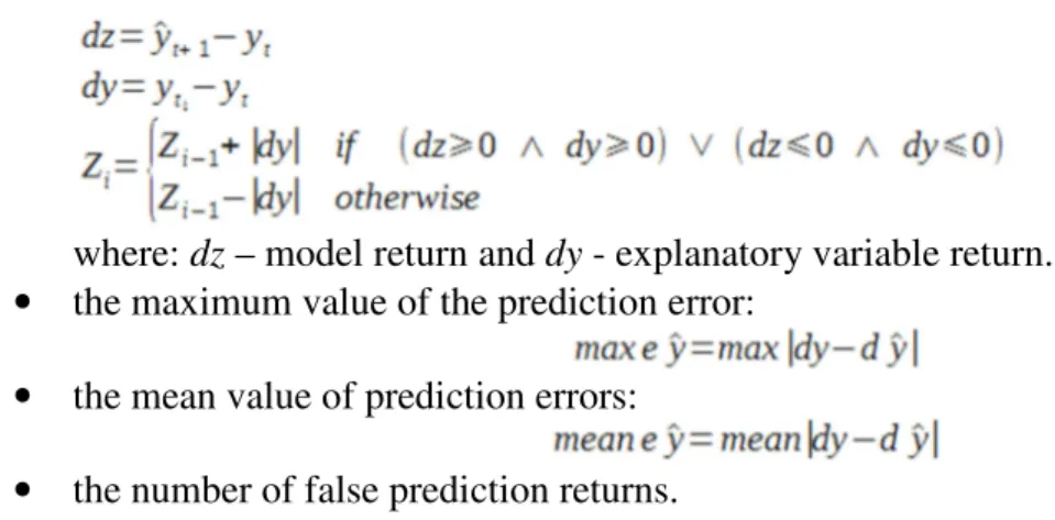
As an indicators of the prediction quality the following measures were used:
• the cumulative sum of profits:
1
Open, High, Low, Close – the values of variable in chosen time period. 2
where: dz – model return and dy - explanatory variable return.
• the maximum value of the prediction error:
• the mean value of prediction errors:
• the number of false prediction returns.
6. Testing forecasting performance, depending on the operation mode
In this study the following parameters were adopted: vector length – 50 candles, time study - 30 candles, the first candle had number 1004 and correspond to the date and time 2009.06.15 16:00, 7 models always were passed to the next layer, prediction horizon was equal hp = 1, the forecasting model was always made by use of the best structure of the sixth layer.
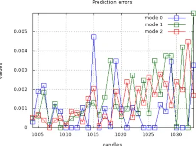
The study clearly shows (figures 2 and 3) that mode 2 gives the best forecasting results. The value of the cumulated sum of profits at the end of the study period reach a value of 0,019, which was a surprising result, because none of other modes were able to achieve sim-ilar result during the test (when this quality indicator was the highest). Mode 1 had the same number of correct decisions as the mode 2 and had similar values of average prediction er-ror. However, other modes had smaller the maximum value of the prediction erer-ror. This reveal the fact that wrong decision can result in large losses. Mode 0 was the weakest strate-gy. The worst result of this strategy could be caused by the fact that the forecast for longer horizon could have bad influence on final decisions. The forecast for long horizon is usually burdened with greater prediction error. The system is misled even when the forecast for shorter horizon is correct. However, it is surprising that this mode had the lowest value of the average prediction error among all modes. In this case, can be postulated that it is the safest strategy that continues to generate profits.
Figure 3. The values of prediction errors made in successive candles received by prediction on one candle ahead and using three modes of operation.
7. Testing forecasting performance, depending on the method of models
selection
In this study the following parameters were adopted: vector length – 50 candles, time study - 30 candles, the first candle had number 1400 and correspond to the date and time 2009.06.19 19:00, 7 models always were passed to the next layer, prediction horizon was equal hp = 1, the forecasting model was always made by use of the best structure of the sixth layer. In the experiment the forecasting system with the use of mode 2 were applied, three computing agents were used, the upper limit of models number is calculated as follow:
Fv=
(
m(m 1)2
)(
Fy(Fy 1)
2
)
L 1
, (3)
where m is the number of explanatory variables, and L is the number of layer. The basic quality criteria for the models was the average of all the model quality values obtained in the first layer. This value was further propagated to the criteria of next layers according to the formula:
CRi=CRi 1∗(1 i∗0.1) , (4)
where i = 2, ..., 6 is a consecutive numbers of layers. The quality of the prediction model was determined based on the accuracy of mapping the actual course of observed variable.
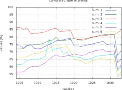
The following methods of models selection was tested: the choice of Fy first models that
meet the criterion (s.m. 1), roulette method (s.m. 2), the selection of Fy the best models (s.m.
3), ranking method (s.m. 4), tournament method (s.m. 5), random selection (s.m. 6).
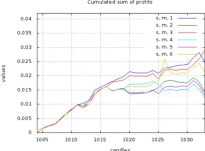
The method based on the selection of Fy the best models (s.m. 3) turned out to be the
best selection method (see figure 4 and 5). This method extends in some way the method consisting in selection of first Fy models that meet the criteria (s.m. 1). The winning method
ensures that the next layer will also include (or rather only) the best models. This is the so-called elitism, which Ivahnenko (creator of the concept of GMDH method) did not want to use. Nevertheless, it appears that the best models obtain the best results.
Of course, in this case the choice of model that goes to the next layer, is a pure coincidence, and it is hard to determine the quality of models, that passed to the next layer. However, we can assume that not only the best models passed to next layer.
The results of simulations, in which were used the selection methods borrowed from the theory of genetic algorithms (s.m. 2, s.m. 4, s.m. 5), show that those methods have a tendency to causing a single, relatively large, errors. In the consequence the cumulative sum of the profit is significantly reduced. However, they do not outperform other methods in terms of the average value of the prediction error. Moreover, they showed a better forecasts accuracy than the other methods. The tournament method (s.m. 5) were the leading among those methods.
Figure 4. The cumulative sum of profits for the subsequent candles received by prediction on one candle ahead and six selection methods
8. Testing forecasting performance, depending on the adopted prediction
horizon and the method of models selection
In this study the following parameters were adopted: vector length – 50 candles, time study - 30 candles, the first candle had number 1400 and correspond to the date and time 2009.06.19 19:00, 7 models always were passed to the next layer, prediction horizon was equal hp = 1, the forecasting model was always made by use of the best structure of the sixth layer. The study was conducted with the use of combinied modes 1 and 2: four computing agents were used, the upper limit of models number can be calculated by use of equation (3). the basic criterion for the quality of the model were the same as in previous experiment.
In this study were tested prediction horizon on two and three candles forward, and the following methods of models selection was tested: the choice of Fy first models that meet
the criterion, roulette method, the selection of Fy the best models, ranking method,
tournament method, random selection.
The method based on the selection of Fy the best models (s.m. 3) outperforms other
methods (see figure 6 and 7). This method achieved the highest results for tested prediction horizons. It has a small value of the maximum prediction error and the average prediction error.
Roulette (s.m. 2) was only slightly less effective. It reaches 70% of maximum profit for studied prediction horizons. It had more than 63% in the effectiveness of the decision making, which is a better result than the s.m. 3 method. Unfortunately, s.m. 2 achieved also the highest values of maximum prediction error and the mean prediction error.
Other selection methods based on the theory of genetic algorithms had much worst results. The worst results had the tournament method (s.m. 5) which had poor results (53 - 64%).
Figure 7. The cumulated sum of profits for the subsequent candles expressed in percentage of maximum profit received by prediction on three candle ahead and using six selection methods.
9. Conclusions
The experimental results reveals that the system is able to produce a reliable investment decisions. As shown in conducted analysis, in spite of the fact that the system makes mis-takes in individual forecasts the cumulative sum of profit is positive.
Presented in this article, time series forecasting system has great potential. These studies demonstrate that the system can be deployed on the trading platform to automate process of the prediction of financial markets. Described in this paper distributed approach extends used by Wiliński [1] GMDH method. It achieves even better results and gives the ability to benefit from distributed computer resources. The proposed changes had a positive influence on the obtained results.
Further research aims at improving an individual forecast and to develop more sophisti-cated investment strategies. The use of more sophistisophisti-cated statistical methods can result in development of better prognostic indicators, which can improve the accuracy of the predic-tion.
References
[1] Wiliński A., GMDH – metody grupowania argumentów w zadaniach zautomatyzowanej pre-dykcji zachowań rynków finansowych, Warszawa - Szczecin 2009, 278 s., ISBN 9788389475237
[2] GMDH - Group Method of Data Handling, http://www.gmdh.net/
[3] Ivakhnenko A., Ivakhnenko G., Problems of Further Development of the Group Method of Data Handling Algorithms, Part I. Pattern Recognition and Image Analysis vol.10 No.2, pp. 187-194, 2000.
[4] Ivakhnenko A., Ivakhnenko G.,Mueller J., Self-organization of Neural Network with Active Neurons, Part I. Pattern Recognition and Image Analysis, vol.4 No.2, pp. 185-196, 1999. [5] Ivakhnenko A.G., Ivakhnenko G.A., Andrienko N.M. Inductive Computer Advisor for Current
[6] Ivakhnenko G.A., Model-Free Analogues As Active Neurons for Neural Networks Self-Organization, Control Systems and Computers, no.2, p.100-107, 2003.
[7] Madala H.R., Ivakhnenko A.G., Inductive Learning Algorithms for Complex Systems Model-ling. CRC Press Inc.. Boca Raton, Ann Arbor, London, Tokyo, ISBN: 0-8493-4438-7, 1994 [8] Rogoza, V., Zabłocki, M., Grid computing and Cloud computing in scope of JADE and OWL
based Semantic Agents – A Survey, Przegląd Elektrotechniczny, 90, 2/2014, ISSN 0033-2097 [9] Bouška J., Kordík P., Time Series Prediction by means of GMDH Analogues Complexing and
GAME (Paper in Conference Proceedings), In IWIM 2007 - International Workshop on Induc-tive Modelling. Praha: Czech Technical University in Prague, 2007, p. 278-287. ISBN 9788001038819
[10] Samsudin R., Saad P., Shabri A., A hybrid least squares support vector machines and GMDH approach for river flow forecasting, Hydrol. Earth Syst. Sci. Discuss., 7, 3691-3731, doi:10.5194/hessd-7-3691-2010, 2010
[11] Kondo T., Kondo Ch., Takao S.,Ueno J.,Feedback GMDH-type neural network algorithm and its application to medical image analysis of cancer of the liver, Artificial Life and Robotics, Volume 15, Issue 3, p. 264-269, 2010