The four modes of supply1

Appendix A-G

A.

Explanation of the modes of supply

………

. p.2

B.

Country coverage in the WIOD and TSD

………

p.3



Includes sector coverage in the TSD

C.

STRI Level and STRI Heterogeneity (score and answer)

……

p.4

D.

Derivation of the input-output framework

………

... p.6

E.

Corresponding tables with the figures in section 3..

……

.

…

.... p.11



Includes sector coverage in the WIOD

F.

Derivation of the theoretical gravity system

………

.. p.17

Appendix A:

The four modes of supply

1.

Cross-border supply of services: when a service supplier resident in one country

provides a service in another country without either supplier or consumer moving to

the physical location.

2.

Consumption abroad: when a consumer resident in one country moves to the location

of a supplier to consume a service.

3.

Commercial presence: when a service provider moves to the location of consumers to

sell services locally through the establishment of a foreign affiliate or branch.

4.

Presence of natural persons: when an individual (temporarily) moves to the country of

the consumers to provide a service.

Appendix B:

Country coverage in the WIOD and TSD

Table A.1

Country and Services Trade Restrictiveness Index (STRI) Coverage

Country TSD & STRI WIOD 2016 Country TSD & STRI WIOD 2016

Australia Yes Yes Japan Yes Yes

Austria Yes Yes Korea Yes Yes

Belgium Yes Yes Latvia Yes Yes

Brazil Yes Yes Luxembourg Yes Yes

Canada Yes Yes Mexico Yes Yes

Chile Yes Yes Netherlands Yes Yes

China No Yes New Zealand Yes Yes

Colombia Yes Yes Norway Yes Yes

Cyprus No Yes Poland Yes Yes

Czech Republic Yes Yes Portugal Yes Yes Denmark Yes Yes Russian Federation Yes Yes

Estonia Yes Yes Slovakia Yes Yes

Finland Yes Yes Slovenia Yes Yes

France Yes Yes South Africa Yes Yes

Germany Yes Yes Spain Yes Yes

Greece Yes Yes Sweden Yes Yes

Hungary Yes Yes Switzerland Yes Yes

Iceland Yes Yes Taiwan No Yes

India Yes Yes Turkey Yes Yes

Indonesia Yes Yes United Kingdom Yes Yes

Ireland Yes Yes United States Yes Yes

Israel Yes Yes Rest of world No Yes

Italy Yes Yes Total 42 45

Notes:

i. All 45 countries (including a model of the Rest of the world) is included in the input-output analysis in section 3, and all 42 countries with a corresponding STRI index is included in the gravity regressions in section 4.

ii. The proportionality assumption2 _{is not applied when creating import matrices for goods and services in}

the WIOD tables, which represent an advantageous feature of the tables because they better reflect the actual trade in intermediates and final goods and services. 3 _{The construction of the tables, however,} allows countries’ import shares to differ across but not within end-use categories.

iii. The construction of the WIOD tables depends on the fixed product sales assumption which implies that for any given industry all firms use the same goods and services to produce the same output.

iv. The TSD provides a consolidated and reconciled version of data from the OECD, Eurostat, IMF and the UN.

v. The TSD is of relative high quality compared to other sources of bilateral trade in services since it has been cross checked across the multiple sources and corrected for inconsistencies and measurement errors (Francois et al., 2013).

2_{The proportionality assumption implies that the share of imports of any given product consumed directly as intermediate consumption or}

final demand (except exports) is the same for all use categories (i.e., industry and category of final demand) (Koopman et al., 2015).

3 _{Dietzenbacher et al. (2013) show that import proportions differ widely across use categories, and within each category they differ by}

Appendix C:

STRI Level and STRI Heterogeneity

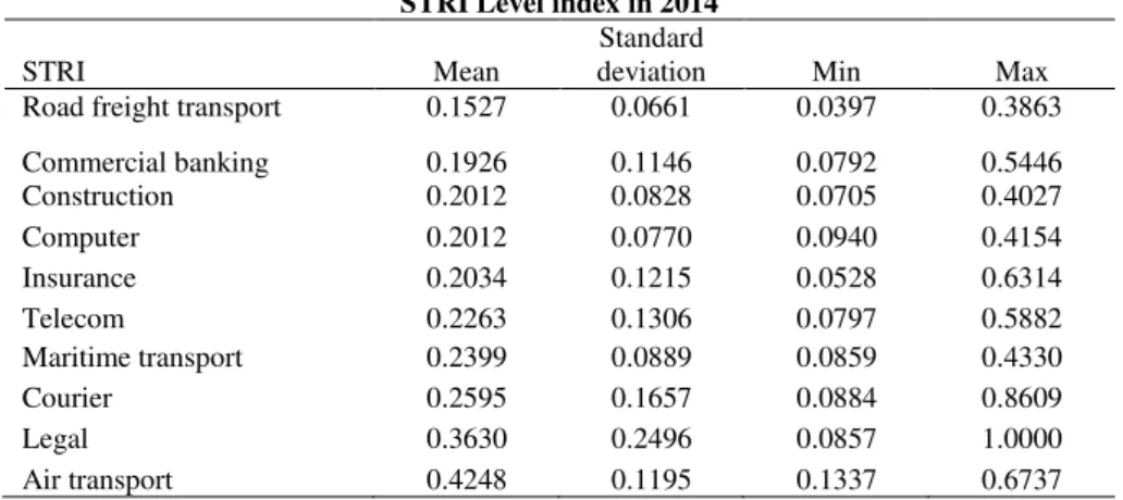
Table C.1 STRI Level index in 2014

STRI Mean

Standard

deviation Min Max Road freight transport 0.1527 0.0661 0.0397 0.3863 Commercial banking 0.1926 0.1146 0.0792 0.5446 Construction 0.2012 0.0828 0.0705 0.4027 Computer 0.2012 0.0770 0.0940 0.4154 Insurance 0.2034 0.1215 0.0528 0.6314 Telecom 0.2263 0.1306 0.0797 0.5882 Maritime transport 0.2399 0.0889 0.0859 0.4330 Courier 0.2595 0.1657 0.0884 0.8609 Legal 0.3630 0.2496 0.0857 1.0000 Air transport 0.4248 0.1195 0.1337 0.6737

Table C.2

STRI Heterogeneity score index in 2014

STRI Heterogeneity score Mean

Standard

deviation Min Max Computer services 0.2498 0.0726 0.0518 0.5643 Construction 0.2447 0.0769 0.0653 0.4786 Legal services 0.3896 0.1743 0 0.8724 Telecommunications 0.3009 0.1256 0.0879 0.6327 Air transport 0.23 0.1438 0.0239 0.5476 Maritime freight transport 0.3018 0.0889 0.0903 0.6433 Road freight transport 0.1831 0.0831 0.0217 0.574 Courier services 0.2311 0.0861 0.0686 0.6111 Commercial banking 0.2379 0.1064 0.0619 0.557 Insurance 0.2347 0.1179 0.0409 0.649

Table C.3

STRI Heterogeneity answer index in 2014

Heterogeneity answer Mean

Standard

deviation Min Max Computer services 0.3114 0.072 0.7784 0.5488 Construction 0.2746 0.0722 0.0847 0.4883 Legal services 0.3108 0.0593 0.1143 0.4746 Telecommunications 0.2811 0.0993 0.0991 0.5929 Air transport 0.1995 0.1085 0.0395 0.5115 Maritime freight transport 0.2874 0.0753 0.1189 0.5338 Road freight transport 0.1872 0.0635 0.0325 0.4259 Courier services 0.2589 0.0733 0.0884 0.4609 Commercial banking 0.2657 0.0999 0.1159 0.6039 Insurance 0.2372 0.1229 0.0635 0.667

Note for Tables C1-C3:

The construction of the STRI Level and STRI Heterogeneity (score and answer)

The construction of the STRI Level is based on a list of standardised questions or measures on

each country’s laws and regulations covering the five policy areas, in which binary scores are

given where answers are simply yes or no, while numerical answers are broken down on

thresholds to which binary scores are applied (Geloso et al., 2015; Nordås, 2016).

The STRI Heterogeneity reflects the (weighted) share of measures for which two countries

have different regulations in a sector. Here, a matrix where each cell contains the answer to a

specific policy measure m by country s and r, which is equal to zero if their answers are the

same and one otherwise. A weighted average of these scores are calculated (same weight to

each measure) and each country and sector are assigned a heterogeneity index. Alternatively,

the heterogeneity index is based on scores assigned to each measure, which are calculated

similarly except that if the country pair in a cell has the same score on measure m, the cell is

also scored zero and one otherwise.

Note that the indices cover restrictions that apply on a most-favoured-nation (MFN) basis,

Appendix D:

Derivation of the input-output framework

The methodology follows the framework in Koopman et al. (2014) and Timmer et al. (2013)

closely.

_{There are G countries and N sectors, each country-sector produces one good or}

service that are absorbed at home or abroad either as a final product or an intermediate input

in production.

_{We further label country-sectors as sources and destinations, where s and r}

denote the source and destination country, and i and j the source and destination sector. We

assume market clearing in the model and equation (D.1) gives the market clearing condition

for a specific product. Here, the value of output in sector i in country s is

𝑋

(𝑖)

, the value of

products exported from sector i in country s for final use in any country r is

𝑌

(𝑖)

, and the

value of goods from sector i in country s for intermediate use by sector j in any country r is

𝑀

(𝑖, 𝑗)

. Note that the use of a product can be bought at home (s=r) or abroad (s≠r).

(D. 1) 𝑋𝑠(𝑖) = ∑ 𝑌𝑠𝑟(𝑖)

𝑟 + ∑ ∑ 𝑀_{𝑟 𝑗} 𝑠𝑟(𝑖, 𝑗)

Then we rewrite the market clearing condition for each GN product in (D.1) to compact form

as

𝑋 = 𝐴𝑋 + 𝑌

, and rearrange terms so that we arrive at the fundamental input-output

condition: (D.2)

𝑋 = (𝐼 − 𝐴)

𝑌 = 𝐵𝑌

. Here, X is as a GN×1 vector of production that

consists of output levels in each country-sector, Y is a GN×1 vector that gives world final

demand for output in each country-sector. The latter is the sum of both domestic and foreign

demand for each country-

sector’s final products, that is,

𝑌

(𝑖) = ∑ 𝑌

(𝑖)

. A denotes the

GN×GN global intermediate input coefficients matrix, where each element

a

(i, j) =

M

(i, j)/X

(j)

reflects sector i’s output (in country s) used as an intermediate input in sector

j’s production (in country r) as a share of total output in the latter sector (in country r). Hence,

A describes how the products of each country-sector are produced using a combination of

both domestic and foreign intermediate inputs.

_The

_{(𝐼 − 𝐴)}

_{term or}

_𝐵

_{is the Leontief}

inverse matrix (Leontief, 1936) with dimension GN×GN, which gives total gross output (both

direct and indirect) required in country s to produce a one-unit increase of final demand in

country r. When multiplying the Leontief inverse matrix with the vector of final demand as in

(D.2), we obtain the necessary production in country s to satisfy demand for final products

absorbed in any country r. Equation (D.2) represents the Inter Country Input-Output (ICIO)

model which can be rewritten as (D.2’) in matrix notation.

4 _{Note that Koopman et al. (2014) do not use their framework to identify sources of added at the country-sector level, but that their}

value-added matrix algebra allows such decomposition.

5 _{A country-sector denotes a particular sector in a country. Final demand consists of household and government consumption and}

investments.

(D.2’) [ X1 X2 ⋮ XG ] = [

I − A11 −A12

−A21 I − A22 … −A 1G

… −A2G

⋮ ⋮

−AG1 −AG2 ⋱

⋮ … I − AGG

]

−1

[ ∑ YGr 1r

∑ YGr 2r

⋮ ∑ YGr Gr]

= [

B11 B12

B21 B22 … B 1G

… B2G

⋮ ⋮

BG1 BG2 ⋱

⋮

… BGG

] [ Y1 Y2 ⋮ YG ]

We

further rewrite equation (D.2’) by breaking up each country’s gross output according to

where it is ultimately absorbed by rearranging all countries’ final demand into a matrix format

by source and destination. That is, the gross output decomposition matrix in equation (D.3).

Domestic production is absorbed at home if s≠r and absorbed abroad if s=r.

With G countries

and N sectors, the gross output decomposition matrix and the final demand matrix are both

GN×G matrices. Similarly, X and Y are both GN vectors. However, equation (D.2)-(D.12)

omits sector notification in order to simplify notation. In expression (D.2),

𝑋

= ∑ 𝑋

is a

N×1 gross output vector that gives gross output produced in s and absorbed in r, and

𝑌

=

∑ 𝑌

is a N×1 final demand vector which gives country r’s demand for final goods produced

in country s.

(D.3) [

X11 X12

X21 X22 … X 1G

… X2G

⋮ ⋮

XG1 XG2 ⋱

⋮

… XGG

] = [

B11 B12

B21 B22 … B 1G

… B2G

⋮ ⋮

BG1 BG2 ⋱

⋮

… BGG

] [

Y11 Y12

Y21 Y22 … Y 1G

… Y2G

⋮ ⋮

YG1 YG2 ⋱

⋮

… YGG

]

We further define

𝑉

as a 1×N value-added coefficient row vector where each coefficient

gives the ratio of direct domestic value-added in total output of country s.

_{This is equal to}

one minus the intermediate input share from all countries (including domestically produced

intermediates).

_{We obtain the value-added share by source (VB) matrix in (D.4) by}

multiplying V, defined as a G×GN diagonal matrix of the domestic value-added for all

countries, with the Leontief inverse matrix (B).

(D.4) VB = [

V1B11 V1B12

V2B21 V2B22 … V 1B1G

… V2B2G

⋮ ⋮

VGBG1 VGBG2 ⋱

⋮ … VGBGG

]

7 _{With G countries and N sectors 𝑉}

𝑠 becomes a 1xGN vector. 8_{Formally, we define 𝑉}

𝑠= 𝑢(𝐼 − ∑ 𝐴𝐺𝑟 𝑟𝑠).

9_{𝑉 = [}

𝑉1 0

0 𝑉2

… 0 … 0 ⋮ ⋮ 0 0 … 𝑉 ⋱ ⋮𝐺

The VB matrix measures value-added share by source of production and reflects the

underlying production structure embedded in the ICIO model. The diagonal elements sum to

domestic value-added share in production, and the off-diagonal column elements sum to

foreign value-added share in the same goods and services. The sum of each row equals unity

since production is either domestic or foreign.

Then we define

𝑉̂

as a diagonal matrix with direct value-added coefficients along the

diagonal, and with G countries and N sectors, we obtain the GN×GN diagonal value-added

coefficient matrix as in equation (D.5).

(D.5) V̂ =

[ V̂1 0

0 V̂2 … 0… 0

⋮ ⋮

0 0 … V̂⋱ ⋮G]

We obtain the GN×G value-added production matrix (

V̂BY

) in equation (D.6) by multiplying

(D.5) with the right hand side of equation (D.3).

(D.6)

[ V̂1 0

0 V̂2 … 0… 0

⋮ ⋮

0 0 … V̂⋱ ⋮G]

[

X11 X12

X21 X22 … X 1G

… X2G

⋮ ⋮

XG1 XG2 ⋱

⋮

… XGG

]

=

[

V̂1∑ B1r G

r Yr1 V̂1∑ B1r

G

r Yr2

V̂2∑ B2r G

r Yr1 V̂2∑ B2r

G

r Yr2

… V̂1∑ B1r

G

r YrG

… V̂2∑ B2r G

r YrG

⋮ ⋮

V̂G∑ BGr G

r Yr1 V̂G∑ BGr

G

r Yr2

_{… V̂}⋱ ⋮

G∑ BGr

G

r YrG]

The

V̂BY

matrix provides estimates of country-sector sources (domestic or foreign) of direct

and indirect value-added used in each country-

sector’s production of final goods consumed at

home or abroad. Diagonal elements reflect countries’

value-added production absorbed at

home, while off-

diagonal elements represent a country’s

value-added exports. We can further

trace backward and forward industrial linkages using the

V̂BY

matrix (Wang, Wi and Zhu,

2013). For instance, we account for a given country-

sector’s

use of domestic value-added by

the sector itself as well as in all downstream country-sectors when summing across a given

row. If we sum the elements in a given column, we take into account the distribution of

value-added from all country-sectors to final goods produced by a particular country-sector. Hence,

we trace forward industrial linkages across all downstream country-

sectors from a producer’s

10 _{Note that 𝑉̂}

perspective when summing across a row, whilst we trace backward industrial linkages across

upstream country-

sector from a user’s perspective when summing along a column (Wang et

al., 2013).

Total value-added exports from country s to the world is defined in Koopman et al. (2014) as

equation (D.7), which we decompose into three components in equation (D.8) according to

where and how the value-added is absorbed ultimately. See section 3.3 for further

explanations.

(𝐷. 7) 𝑉𝑇𝑠∗ = ∑ 𝑉 𝐺

𝑟≠𝑠

𝑋𝑠𝑟= 𝑉𝑠∑ ∑ 𝐵𝑠𝑔𝑌𝑔𝑟 𝐺

𝑔=1 𝐺

𝑟≠𝑠

(D. 8) 𝑉𝑇𝑆∗= 𝑉𝑠∑ 𝐵𝑠𝑠 𝐺

𝑟≠𝑠

𝑌𝑠𝑟+ 𝑉𝑠∑ 𝐵𝑠𝑟 𝐺

𝑟≠𝑠

𝑌𝑟𝑟+ 𝑉𝑠∑ ∑ 𝐵𝑠𝑟𝑌𝑟𝑡 𝐺

𝑡≠𝑠,𝑟 𝐺

𝑟≠𝑠

(D. 9) 𝐸𝑠∗= ∑ 𝐸𝑠𝑟 𝐺

𝑟≠𝑠

∑(𝐴𝑠𝑟𝑋𝑟+ 𝑌𝑠𝑟) 𝐺

𝑟≠𝑠

Equation (D.9) reflects a country’s gross exports to the world and includes exports of

intermediates and final goods. Koopman et al. (2014) further decompose gross exports in

equation (D.9) into nine components that identify foreign and domestic sources of

value-added as well as double-counted trade, equation (D.10) gives the decomposition formula.

(D. 10) 𝑢𝐸𝑠∗ = {𝑉𝑠∑ 𝐵𝑠𝑠𝑌𝑠𝑟+ 𝑉𝑠∑ 𝐵𝑠𝑟𝑌𝑟𝑟 𝐺

𝑟≠𝑠

+ 𝑉𝑠∑ ∑ 𝐵𝑠𝑟𝑌𝑟𝑡 𝐺 𝑡≠𝑠,𝑟 𝐺 𝑟≠𝑠 𝐺 𝑟≠𝑠 }

+ {𝑉𝑠∑ 𝐵𝑠𝑟𝑌𝑟𝑠+ 𝑉𝑠∑ 𝐵𝑠𝑟𝐴𝑟𝑠(𝐼 − 𝐴𝑠𝑠)−1𝑌𝑠𝑠 𝐺

𝑟≠𝑠 𝐺

𝑟≠𝑠

}

+ 𝑉𝑠∑ 𝐵𝑠𝑟𝐴𝑟𝑠(𝐼 − 𝐴𝑠𝑠)−1𝐸𝑠∗ 𝐺

𝑟≠𝑠

{∑ ∑ 𝑉𝑡𝐵𝑡𝑠𝑌𝑠𝑟 𝐺

𝑟≠𝑠

+ ∑ ∑ 𝑉𝑡𝐵𝑡𝑠𝐴𝑠𝑟(𝐼 − 𝐴𝑟𝑟)−1𝑌𝑟𝑟 𝐺 𝑟≠𝑠 𝐺 𝑡≠𝑠 𝐺 𝑡≠𝑠 }

+ ∑ 𝑉𝑡𝐵𝑡𝑠𝐴𝑠𝑟∑(𝐼 − 𝐴𝑟𝑟)−1𝐸𝑟∗ 𝐺

𝑟≠𝑠 𝐺

𝑡≠𝑠

The three first terms are value-added exports as defined in equation (D.9). The fourth and the

fifth terms, in the second bracketed expression, include the source country’s

value-added in

both its final and intermediate goods imports, which are first exported but eventually returned

and consumed at home, both of which are parts of the source country’s GDP but represent a

double-counted portion in official gross export statistics. These six terms together reflect the

value-added exports because they are not consumed abroad. The seventh and eight term in the third

bracketed expression represent foreign value-added

(GDP) in the source country’s gross

exports, including foreign GDP embodied in both final and intermediate goods. There are

two pure double-counted terms, the sixth and ninth terms sum up to the double-counted

portions of the two-way intermediate trade from all bilateral routes (third partners). Note that

equation (D.10) does not hold at the country-sector level, therefore it is not emphasized in the

analysis.

Koopman et al. (2014) define backward vertical specialisation in country s (

𝑉𝑆

) as equation

(D.11) and forward vertical specialisation (

𝑉𝑆1

) as equation (D.12).

(D. 11) 𝑉𝑆𝑠 = ∑ ∑ 𝑉𝑡𝐵𝑡𝑠𝑌𝑠𝑟 𝐺

𝑟≠𝑠

+ ∑ ∑ 𝑉𝑡𝐵𝑡𝑠𝐴𝑠𝑟(𝐼 − 𝐴𝑟𝑟)−1𝑌𝑟𝑟 𝐺

𝑟≠𝑠 𝐺

𝑡≠𝑠 𝐺

𝑡≠𝑠

+ ∑ 𝑉𝑡𝐵𝑡𝑠𝐴𝑠𝑟∑(𝐼 − 𝐴𝑟𝑟)−1𝐸𝑟∗ 𝐺

𝑟≠𝑠

𝐺

𝑡≠𝑠

(D. 12) 𝑉𝑆1𝑠 = 𝑉𝑠∑ 𝐵𝑠𝑟𝐸𝑟∗ 𝐺

𝑟≠𝑠

= 𝑉𝑠∑ ∑ 𝐵𝑠𝑟𝑌𝑟𝑡 𝐺

𝑡≠𝑠,𝑟 𝐺

𝑟≠𝑠

+ 𝑉𝑠∑ ∑ 𝐵𝑠𝑟𝐴𝑟𝑡𝑋𝑡 𝐺

𝑡≠𝑠,𝑟 𝐺

𝑟≠𝑠

+ 𝑉𝑠∑ 𝐵𝑠𝑟𝑌𝑟𝑠 𝐺

𝑟≠𝑠

+ 𝑉𝑠∑ 𝐵𝑠𝑟𝐴𝑟𝑠𝑋𝑠 𝐺

𝑟≠𝑠

VS measures the share of foreign inputs in either a country’s total gross exports or a country

-sector’s gross exports. The first and second components are

foreign value-added in exports of

final products and intermediates, respectively, and the third term reflects double-counted

intermediate exports produced abroad. Koopman et al. (2014) generalise VS measure in

Hummels et al. (2001) to fit a multi-country setting with unrestricted intermediate goods

trade.

Furthermore, Koopman et al.

(2014) define VS1 as the share of a given country’s

exports of intermediates used as inputs by foreign countries to produce final exports to third

countries. Note that equation (D.12) does not hold at the country-sector level, therefore it is

not emphasized in the analysis.

11_{The generalisation by Koopman et al. (2014) is done by allocating double-counted intermediates in gross exports to domestic or foreign}

Appendix E:

Corresponding tables to figures in section 3 and sector overview in the

WIOD 2016

Table E.1. Sector overview in the WIOD 2016,

Gross and value-added exports and vertical specialization (VS) by sector

Gross exports Value-added exports Vertical specialisation (VS)

Sector description ISIC

Rev. 4

WIOD sector

2000 2014 2000 2014 2000 2014

Crop and animal production, hunting and related service activities

A01 c1 48.94 164.01 480.58 825.41 0.13 0.19

Forestry and logging A02 c2 22.47 198.14 347.46 294.80 0.06 0.09

Fishing and aquaculture A03 c3 1179.05 5410.34 1053.40 3460.59 0.13 0.17

Mining and quarrying B c4 37784.10 90073.77 34904.71 79962.75 0.03 0.08

Total primary sector excluding Mining and quarrying c1-c3 1250.46 5772.49 1881.44 4580.81 0.13 0.17

Manufacture of food products, beverages and tobacco products

C10-C12 c5 2920.93 6781.39 1103.19 2994.13 0.14 0.20

Manufacture of textiles, wearing apparel and leather products

C13-C15 c6 278.98 378.78 223.18 336.03 0.18 0.20

Manufacture of wood and of products of wood and cork, except furniture; manufacture of articles of straw and plaiting materials

C16 c7 376.07 405.68 226.95 281.45 0.20 0.22

Manufacture of paper and paper products C17 c8 1432.39 1018.70 648.70 383.93 0.19 0.21

Printing and reproduction of recorded media C18 c9 21.07 24.07 148.47 168.95 0.22 0.19

Manufacture of coke and refined petroleum products C19 c10 2352.39 7015.35 692.27 1220.05 0.27 0.24

Manufacture of chemicals and chemical products C20 c11 2073.12 5605.12 666.77 895.98 0.27 0.24

Manufacture of basic pharmaceutical products and pharmaceutical preparations

C21 c12 392.75 1382.98 104.76 216.69 0.27 0.24

Manufacture of rubber and plastic products C22 c13 330.98 670.64 186.96 406.10 0.26 0.30

Manufacture of other non-metallic mineral products C23 c14 310.48 559.11 228.63 525.70 0.19 0.21

Manufacture of basic metals C24 c15 4521.14 8341.86 1988.18 2043.71 0.34 0.42

Manufacture of fabricated metal products, except machinery and equipment

C25 c16 590.13 2020.11 633.77 2174.70 0.22 0.25

Manufacture of computer, electronic and optical products C26 c17 1562.77 3281.50 897.63 1734.05 0.26 0.25

Manufacture of electrical equipment C27 c18 686.99 1998.58 360.22 1010.89 0.28 0.31

Manufacture of machinery and equipment n.e.c. C28 c19 1647.34 6667.78 717.06 3440.88 0.29 0.31

Manufacture of motor vehicles, trailers and semi-trailers C29 c20 561.31 965.81 251.85 394.42 0.29 0.33

Manufacture of other transport equipment C30 c21 1623.03 2723.26 904.13 1218.02 0.30 0.31

Manufacture of furniture; other manufacturing C31_C32 c22 564.31 785.24 381.99 517.87 0.18 0.22

Repair and installation of machinery and equipment C33 c23 198.88 1053.72 329.31 1601.09 0.29 0.26

Total manufacturing sector c5-c23 22445.07 51679.68 10694.02 21564.61 0.26 0.28

Electricity, gas, steam and air conditioning supply D35 c24 579.36 779.59 1017.77 2530.26 0.06 0.06

Water collection, treatment and supply E36 c25 0.15 0.42 7.64 20.20 0.10 0.14

Sewerage; waste collection, treatment and disposal activities; materials recovery; remediation activities and other waste management services

E37-E39 c26 162.01 892.42 459.43 800.71 0.12 0.20

Notes:

i. Exports in million current US dollars.

ii. The aggregated sectors primary, manufacturing and service are defined according to ISIC Rev. 4 Divisions 1-3, 5-23, 27-56, respectively. Note that Mining and quarrying (Division 4) is excluded in the primary sector.

iii. In section 3.4 we divide services sectors into broader categories: Construction (27), Wholesale and retail trade (including repair of motor vehicles and motorcycles) (28-30), Water transportation (32), Transportation and storage (31, 33-35), Accommodation and food service activities (36), Information and communication (37-40), Financial and insurance activities (41-43), Real estate activities (44) and Professional, scientific and technical activities (45-49).

Table E.1. (cont.)

Gross exports Value-added exports Vertical specialisation (VS)

Description ISIC

Rev. 4

WIOD sector

2000 2014 2000 2014 2000 2014

Construction F c27 125.11 307.51 311.28 865.48 0.19 0.20

Wholesale and retail trade and repair of motor vehicles and motorcycles

G45 c28 4.39 31.62 496.94 1132.85 0.18 0.20

Wholesale trade, except of motor vehicles and motorcycles

G46 c29 42.97 199.86 1657.01 3582.43 0.12 0.17

Retail trade, except of motor vehicles and motorcycles G47 c30 199.71 717.16 1187.90 2970.48 0.11 0.13

Land transport and transport via pipelines H49 c31 1471.18 2287.56 1498.11 2636.70 0.13 0.17

Water transport H50 c32 7828.08 15622.04 3006.45 7324.92 0.24 0.32

Air transport H51 c33 444.10 1456.35 362.03 667.19 0.20 0.38

Warehousing and support activities for transportation H52 c34 514.83 1749.23 630.45 2103.92 0.22 0.29

Postal and courier activities H53 c35 68.29 328.02 291.16 432.20 0.08 0.13

Accommodation and food service activities we c36 10.03 48.27 160.67 427.75 0.10 0.13

Publishing activities J58 c37 30.13 146.23 231.96 618.13 0.12 0.13

Motion picture, video and television programme production, sound recording and music publishing activities; programming and broadcasting activities

J59_J60 c38 41.00 97.70 65.04 266.50 0.14 0.18

Telecommunications J61 c39 287.91 1019.86 343.19 1125.06 0.15 0.14

Computer programming, consultancy and related activities; information service activities

J62_J63 c40 258.61 1728.14 338.10 1890.29 0.11 0.12

Financial service activities, except insurance and pension funding

K64 c41 301.46 1866.75 866.27 4135.85 0.05 0.06

Insurance, reinsurance and pension funding, except compulsory social security

K65 c42 110.67 343.51 79.14 652.98 0.09 0.05

Activities auxiliary to financial services and insurance activities

K66 c43 87.93 613.57 277.71 575.34 0.03 0.17

Real estate activities L68 c44 2.87 49.21 769.65 2285.18 0.07 0.08

Legal and accounting activities; activities of head offices; management consultancy activities

M69_M70 c45 119.07 1476.49 340.12 1889.17 0.08 0.09

Architectural and engineering activities; technical testing and analysis

M71 c46 738.24 2715.75 401.49 2021.60 0.16 0.17

Scientific research and development M72 c47 80.85 146.60 63.28 117.57 0.10 0.09

Advertising and market research M73 c48 59.75 722.78 122.32 402.05 0.22 0.27

Other professional, scientific and technical activities; veterinary activities

M74_M75 c49 353.57 1346.00 215.71 852.13 0.18 0.18

Administrative and support service activities N c50 480.69 3007.65 1005.78 4360.25 0.15 0.18

Public administration and defence; compulsory social security

O84 c51 112.16 161.89 1526.58 984.85 0.08 0.09

Education P85 c52 0.79 127.87 122.21 239.71 0.04 0.05

Human health and social work activities Q c53 127.64 427.39 141.11 533.37 0.06 0.06

Other service activities R_S c54 46.57 187.28 194.94 563.91 0.10 0.13

Activities of households as employers; undifferentiated goods- and services-producing activities of households for own use

T c55 0.00 0.00 0.00 0.00 0.00 0.00

Activities of extraterritorial organizations and bodies U c56 0.00 0.00 0.00 0.00 0.00 0.00

Table E.2

Decomposition of value-added by origin and double-counted elements in gross exports

2000 2014

(1) Domestic VA in direct final goods 17.07 12.03 (2) Domestic VA in intermediates absorbed by direct importer 57.30 58.10 (3) Indirect VA exports to third countries 11.85 12.32

Value-added exports (1)-(3) 86.22 82.45

(4) Returned domestic VA in final goods 0.22 0.21 (5) Returned domestic VA in intermediate goods 0.20 0.29 (6) Pure double-counting in returned intermediates 0.22 0.25

Domestic VA embodied in gross exports (1)-(5) 86.64 82.96 (7) Foreign VA in final goods 3.85 3.57 (8) Foreign VA in intermediate goods 5.22 7.30 (9) Pure double-counting in foreign intermediates 4.05 5.91

Pure double-counted terms (6)+(9) 4.27 6.16

Foreign VA used in production of exports absorbed abroad (7)+(8)

9.08 10.87

Sum (1)-(9) 100.0 100.0

% share in gross exports.

Table E.3

Participation in global value chains

Year Total GVC participation

Forward participation (VS1)

Backward participation (VS)

2000 50.33 37.20 13.13

2001 50.65 36.23 14.41

2002 50.59 36.37 14.22

2003 52.20 37.56 14.65

2004 53.48 38.91 14.57

2005 55.21 41.30 13.90

2006 57.75 43.93 13.82

2007 58.47 42.40 16.07

2008 62.02 47.95 14.07

2009 56.53 40.96 15.57

2010 60.78 44.28 16.51

2011 64.40 48.78 15.61

2012 64.86 49.38 15.47

2013 62.08 45.92 16.16

2014 62.07 45.29 16.78

Table E.4

Exports of the primary, manufacturing and service sectors Primaries including

Mineral and quarrying

Primary sector Manufacturing sector Service sector

Year Gross exports

Value-added exports

Intermedi-ate exports

Gross exports

Value-added exports

Intermedi-ate exports

Gross exports

Value-added exports

Intermedi-ate exports

Gross exports

Value-added exports

Intermedi-ate exports

2000 39034.56 36786.15 35714.70 1250.46 1881.44 388.05 22445.07 10694.02 14719.52 13948.59 16706.63 9132.10

2001 37268.22 34225.77 33161.39 1024.05 1641.44 343.72 23202.62 11003.44 14517.76 14729.62 17662.24 9641.24

2002 36553.94 33259.13 33483.01 1086.73 1664.09 301.83 23803.69 11444.81 15094.64 15633.38 18887.63 10216.39

2003 41799.20 37753.61 38190.74 1256.79 1617.41 217.08 27276.81 13071.58 17817.53 17356.87 21043.53 12533.15

2004 53006.16 49108.18 48299.24 1481.51 1930.36 146.17 30983.74 14257.41 21189.75 20185.94 23602.03 14453.82

2005 69859.92 65975.62 65101.48 1955.50 2392.32 487.96 35858.01 15694.64 24701.51 23345.56 26889.08 15982.34

2006 82043.49 77510.54 76554.50 2444.83 2676.94 486.22 42248.54 17938.10 29585.57 24810.47 29887.39 17067.84

2007 86065.66 79194.60 78543.13 2798.39 2746.01 1050.52 52342.20 21247.02 37144.16 29206.82 37039.29 21032.09

2008 117758.45 108340.93 110385.68 3114.62 2914.59 1228.82 57565.73 23986.51 39599.01 33170.52 42463.68 23718.48

2009 74878.61 65492.40 70009.15 3318.53 3019.39 1058.72 44881.84 19008.98 29334.80 26807.67 36436.53 19700.21

2010 86127.96 75096.68 80332.56 4276.87 3982.21 1857.61 47366.36 20338.83 31900.67 31165.56 38641.73 23119.67

2011 109833.57 100328.76 106043.55 4124.86 3788.53 1878.53 55062.06 21888.59 37757.05 33648.15 41604.51 24523.10

2012 113017.53 101485.09 106073.88 4019.70 3088.76 1072.27 51344.83 20825.63 35355.29 35390.24 42789.50 26144.44

2013 107648.06 94772.74 104292.80 5596.06 4165.00 2769.93 51505.42 21488.07 34932.11 38639.24 45663.98 29863.22

2014 95846.26 84543.56 92259.58 5772.49 4580.81 3136.05 51679.68 21564.61 34711.40 38932.28 45657.89 30231.85

Notes:

i. Exports in million current US dollars.

ii. The aggregated sectors primary, manufacturing and service are defined according to ISIC Rev. 4 Divisions 1-3, 5-23, 27-56, respectively. iii. Note that Mining and quarrying (Division 4) is excluded in the Primary sector.

iv. Since the information in WIOD is based on industries and not tasks, and many manufacturing firms produce significant in-house services, the latter activities are not classified under services categories in the data used to construct WIOD tables but as industry output. As a result, estimates of the services content of manufactured goods (based on industries) may underestimate the true underlying value-added from services based tasks (OECDb, 2015).

Figure E.1

Exports of Primary sector goods including the Mining and quarrying sector

0 20000 40000 60000 80000 100000 120000

2000 2001 2002 2003 2004 2005 2006 2007 2008 2009 2010 2011 2012 2013 2014

E

xp

o

rts i

n

mi

ll

ion

cu

rre

n

t

U

S

d

o

ll

ars

Gross exports of primary sector goods including Mineral and quarrying

Table E.5

Decomposition of value-added (VA) exports by aggregated sector

Primary Manufacturing Services

2000 2014 2000 2014 2000 2014

Total VA exports 1881.44 4580.81 10694.02 21564.61 16706.63 45657.89 Domestic VA in direct final goods 63.06 51.42 34.80 34.91 32.36 22.28 Domestic VA in intermediates absorbed by direct

importer

27.60 40.89 49.76 50.33 54.76 64.72 Indirect VA exports to third countries 9.34 7.68 15.44 14.76 12.88 13.00

% share in total value-added exports of aggregate sector.

Table E.6

Value-added share of domestic and foreign services in gross exports

2000 2014

VA from domestic services in gross exports 22.05 24.43 VA from foreign services in gross exports 6.10 8.51 VA from domestic services in manufacturing gross exports 21.14 18.90 VA from foreign services in manufacturing gross exports 9.73 11.99

% share in total gross exports or manufacturing gross exports.

Notes for Table E.6:

i. See note (iv) and (v) under Table E.4.

Table E.7

Sector shares in world total value-added and gross exports

Share in gross exports Share in value-added exports 2000 2014 2000 2014 Primary 0.08 0.11 0.11 0.16 Manufacturing 0.66 0.61 0.41 0.36 Services 0.25 0.27 0.44 0.45

% share in world total gross and value-added exports.

Notes for Table E.7:

i. Corresponds to Figure 1.1 in section 1 of the study. ii. Exports in million current US dollars.

Appendix F:

Derivation of the theoretical gravity system by Anderson and van Wincoop (2003)

The Anderson and van Wincoop model assumes that goods are differentiated by place of

origin

_{, that each country is specialised in the production of one good while the supply of}

goods is fixed. Market clearance is imposed by the general-equilibrium structure of the model.

Consumers have homothetic preferences over all goods that are identical across countries.

Preferences are approximated by the constant elasticity of substitution (CES) utility function

given in equation (F.1), which consumers in country r maximize subject to the budget

constraint in equation (F.2).

(F. 1) (∑ 𝛽𝑠(1−𝜎)/𝜎𝑐𝑠𝑟(𝜎−1)/𝜎 𝑠

)

(𝜎−1)/𝜎

𝑠. 𝑡. (F. 2) ∑ 𝑝𝑠𝑟𝑐𝑠𝑟 𝑠

= 𝑦𝑟

Where

𝑐

is consumption by consumers in country r of goods from country s;

𝑦

is nominal

income of country r;

𝜎 > 0

is the elasticity of substitution between all goods and referred to

as the trade elasticity; whilst

𝛽

is a positive distribution parameter. Prices differ between

home and abroad due to not directly observable trade costs;

𝑝

is the price consumers in

country r pay for goods from country s;

𝑝

is the supply price given by the exporter in country

s (net of trade costs); and

𝑡

is the trade cost of exporting a good from country s to country r;

thus

𝑝

= 𝑝

𝑡

. The exporter carries the trade cost {

𝑡

} which is equal to

𝑡

− 1

(where

𝑡

≥ 1

) for each good from country s shipped to country r. These trade costs are passed on to

the importer from the exporter. Thus, we can write the nominal value of exports from s to r as

𝑥

= 𝑝

𝑐

= 𝑝

𝑡

𝑐

. Note that trade costs are modelled according the structure of iceberg

costs, which assumes that only a fraction {

𝑡

∈ (0.1)

} of the good shipped arrives at

destination, the rest having melted in transit. Finally, we define total income of country s as

𝑦

= ∑ 𝑥

.

Maximization of (F.1) subject to (F.2) results in the nominal demand consumers in country r

have for goods produced in country s as in equation (F.3).

𝑃

is the consumer price index of

country r given by equation (F.4).

𝛽

can be interpreted as an inverse measure of quality, for

instance, a higher

𝛽

implies a lower demand in country r for goods from country s. Market

clearing is imposed by

the model’s general

-equilibrium structure, and as shown in equation

(F.5), it implies that the sum of exports from country s to all destinations, including itself,

equals the total value of production in country s, which in aggregate is

𝑦

.

(F. 3) 𝑥𝑠𝑟= (𝛽𝑠𝑝_𝑃𝑠_𝑟𝑡𝑠𝑟) (1−𝜎)

𝑦𝑟 where (F. 4) 𝑃𝑟= [∑ (𝛽𝑠 𝑠𝑝𝑠𝑡𝑠𝑟)1−𝜎]1/(1−𝜎)

(F. 5) 𝑦𝑠= ∑ 𝑥𝑟 𝑠𝑟= ∑ (𝛽𝑠𝑡_𝑃𝑠𝑟_𝑟𝑝𝑠) 1−𝜎

𝑟 𝑦𝑟= (𝛽𝑠𝑝𝑠)1−𝜎∑ (𝑡_𝑃𝑠𝑟_𝑟)

1−𝜎

𝑟 𝑦𝑟 ∀𝑠

We obtain equation (F.6) by inserting the demand function in (F.3) into the market clearing

condition

𝑦

= ∑ 𝑥

and solve for

(𝛽

𝑝

)

.

(F. 6) (𝛽𝑠𝑝𝑠)1−𝜎= 𝑦𝑠

∑ (𝑡𝑠𝑟

𝑃𝑟) 1−𝜎

𝑦𝑟 𝑟

We define world nominal income or world GDP as

𝑦

= ∑ 𝑦

, and expand the right hand

side of equation (F.6) with

(1/𝑦

) × (1/𝑦

)

, which gives:

(F. 7) 𝑥𝑠𝑟= (𝑡_𝑃𝑠𝑟 𝑟)

1−𝜎_𝑦

𝑟𝑦𝑠

𝑦𝑤 [∑ (

𝑡𝑖𝑗

𝑃𝑟) 1−𝜎

𝑟

𝑦𝑟

𝑦𝑤] −1

We obtain the Anderson and van Wincoop gravity equation in (F.8) after some rearranging of

equation (F.7), where

𝜋

and

𝑃

are the multilateral resistance terms defined in equations

(F.9) and (F.10). Equation (F.9) is obtained by expanding the right hand side of equation (F.6)

by

(1/𝑦

) × (1/𝑦

)

, substituting the resulting expression into the price index in (F.4) and

inserting for

𝜋

.

(F.8) 𝑥_𝑠𝑟=𝑦𝑠𝑦𝑟

𝑦𝑤 (

𝑡𝑠𝑟

𝜋𝑠𝑃𝑟)

1−𝜎

(F.9) 𝜋_𝑠1−𝜎= ∑ (𝑡𝑠𝑟

𝑃𝑟)

1−𝜎 𝑦𝑟

𝑦𝑤

𝑟

(F. 10) 𝑃𝑟1−𝜎= ∑ (𝑡_𝜋𝑠𝑟 𝑠)

1−𝜎

𝑠

𝑦𝑠

𝑦𝑤

The trade cost term in (F.7) is not directly observable and Anderson et al (2003) use equation

(F.11) as a proxy for trade costs, where

𝑑

is bilateral distance and

𝐵

equals one if two

trade partners share an international border.

Appendix G:

Summary statistics and additional regression tables from the gravity analysis in section

4

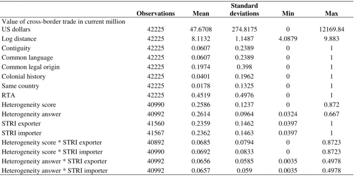
Table G.1 Summary statistics

Observations Mean

Standard

deviations Min Max

Value of cross-border trade in current million

US dollars 42225 47.6708 274.8175 0 12169.84

Log distance 42225 8.1132 1.1487 4.0879 9.883

Contiguity 42225 0.0607 0.2389 0 1

Common language 42225 0.0607 0.2389 0 1

Common legal origin 42225 0.1974 0.398 0 1

Colonial history 42225 0.0401 0.1962 0 1

Same country 42225 0.0178 0.1325 0 1

RTA 42225 0.4519 0.4976 0 1

Heterogeneity score 40990 0.2586 0.1237 0 0.872 Heterogeneity answer 40992 0.2614 0.0964 0.0324 0.667

STRI exporter 41560 0.2359 0.1462 0.0397 1

STRI importer 41567 0.2362 0.1463 0.0397 1

Heterogeneity score * STRI exporter 40892 0.0685 0.0794 0 0.8723 Heterogeneity score * STRI importer 40990 0.0692 0.0833 0 0.8723 Heterogeneity answer * STRI exporter 40992 0.0656 0.0585 0.0035 0.4978 Heterogeneity answer * STRI importer 40992 0.0657 0.059 0.0035 0.4978

Table G.2

Number of observations, missing observations and reported zeroes by sector

Correspondence between EBOPS 2002 & STRI sector Includes missing values Excludes missing values EBOPS 2002 STRI sector Zeroes (%) Missing (%) Observations Zeroes (%)

262bc _{Computer services 27.58 14.91 4396 32.42}

249b _{Construction 31.57 7.86 4760 34.26}

275b _{Legal services 38.71 22.22 4018 49.78}

247b _{Telecommunications 32.71 16.94 4291 39.38}

210 Air transport 21.43 20.11 4127 26.82

208 Maritime freight transport 30.68 22.36 4011 39.52 225 Road freight transport 33.26 26.50 3797 45.25

246c _{Courier services 51.14 20.89 4087 64.64}

260c _{Commercial banking 31.38 16.49 4314 37.58}

253c _{Insurance 33.51 14.36 4424 39.13}

i. Column 3 and 4 report the percentage shares of zeroes and missing values in a balanced panel with 5166 observations in each sector, that is, sectoral bilateral trade is included although the observations are missing. Column 5 and 6 report the number of observations and the percentage share of zeroes when missing values are set to zero. Note that Francois et al (2013) state that unreported exporter:importer:bop:year combinations can safely be assumed as missing in the TRD, while reported zeroes mean that at least one primary source (UN, OECD, Eurostat, IMF) reported a zero flow rather than missing.

ii. STRI indices are available in both 2014 and 2015.

Sector specific regressions

Table G.3 and G.4 provide the sector regressions for those sectors with a STRI heterogeneity

index available in two years. The estimates of the sector regressions tend to be more arbitrary,

which could be due to few observations according to “gravity standards”. Note that I excluded

the coefficients for common language and colony since the other gravity coefficients performed

better that way. Additionally, I include an EEA dummy as well as a RTA dummy since the

European Economic Areas (EEA) is one of the most integrated agreements on trade in services.

As pointed out in Nordås (2016), there are few other regional or preferential trade agreements

than the EU and EEA that bind measures below applied Most Favored Nation (MFN) regulation.

Therefore, the EEA dummy could capture preferential harmonization that is not captured by

the STRI heterogeneity index as the latter only captures MFN regulations, in addition to other

benefits and commonalities that come with the membership. The EEA dummy is equal to one

for country pairs where both are members of the EEA. The estimates of distance are negative

and statistically significant at least at 10 percent levels, common legal origin and same country

are positive and statistically significant at least at 5 percent levels for computer, construction

and telecommunications. However, the estimates of the RTA, EEA and heterogeneity indices

do not perform well since, in general, they have contradictory signs and unreasonable high

magnitudes. Table G.5 and G.6 provide estimates for ten services sectors where I have used

observation from three years and assumed the STRI heterogeneity index to be constant over the

period, to obtain more observations. Nevertheless, the results seem even more arbitrary here,

for instance, some of the gravity coefficients have contradictory signs even if they are

Table G.3

PPML sector regressions, STRI Heterogeneity score

(1) (2) (3) (4)

Computer services

Construction Legal services Telecommuni-cations Log distance -0.285*** -0.437*** -0.0996* -0.815***

(0.0911) (0.0774) (0.0518) (0.0719) Contiguity 0.0337 0.0879 0.904*** 0.158

(0.145) (0.124) (0.149) (0.0978) Common legal origin 0.319*** 0.291*** -0.200 0.603***

(0.123) (0.104) (0.162) (0.0622) Same country 0.671*** 0.692*** -0.0114 0.327** (0.191) (0.263) (0.248) (0.144) RTA 0.575*** 77.7 0.670** 95.4 1.619*** 404 -1.214***

(0.216) (0.332) (0.292) (0.276) EEA-intra 0.864** 137.3 -0.269 -23.2 -0.467 1.874***

(0.341) (0.371) (0.392) (0.314) Heterogeneity score -2.190*** -88.8 1.336 1.798*** -0.790 (0.682) (0.857) (0.626) (0.760) Exporter-year and

importer-year FEs

Yes Yes Yes Yes

Observations 2,878 3,280 2,622 2,800

Pseudo-R2 _{0.796 0.498 0.820 0.846}

(i) The dependent variable is bilateral trade in services by sector in 2008 and 2009. (ii) Robust standard errors clustered by country pair in parentheses.

(iii) ***, ** and * denote significance at 1, 5 and 10 % levels, respectively.

Table G.4

PPML sector regressions, STRI Heterogeneity answer

(1) (2) (3) (4)

Computer services

Construction Legal services Telecommuni-cations Log distance -0.295*** -0.471*** -0.0755 -0.818***

(0.0895) (0.0781) (0.0520) (0.0724) Contiguity -0.0610 0.111 0.924*** 0.156

(0.130) (0.124) (0.154) (0.0972) Common legal origin 0.345*** 0.298*** -0.289* 0.618***

(0.125) (0.104) (0.175) (0.0637) Same country 0.722*** 0.669*** -0.0348 0.335** (0.190) (0.258) (0.245) (0.145) RTA 0.761*** 0.620* 1.557*** -1.225***

(0.230) (0.330) (0.289) (0.278) EEA-intra 0.682** -0.284 -0.341 1.882***

(0.332) (0.376) (0.403) (0.321) Heterogeneity answer -1.214 3.333*** 1.233* -0.401 (0.940) (1.111) (0.704) (0.844) Exporter-year and

importer-year FEs

Yes Yes Yes Yes

Observations 2,878 3,280 2,622 2,800

Pseudo-R2 _{0.772 0.499 0.813 0.845}

(i) The dependent variable is bilateral trade in services by sector in 2008 and 2009. (ii) Robust standard errors clustered by country pair in parentheses.

Table G.5

PPML sector regressions, STRI Heterogeneity score

(1) (2) (3) (4) (5) (6) (7) (8) (9) (10)

Computer services

Construction Legal services Telecommuni-cations

Air transport

Maritime transport

Road transport

Courier Commercial banking

Insurance

Log distance -0.327*** -0.463*** 0.242** -0.866*** -0.223*** -0.163* -0.349*** -0.342* -0.744*** 0.356*** (0.0708) (0.0716) (0.101) (0.0874) (0.0684) (0.0962) (0.0805) (0.206) (0.0822) (0.116) Contiguity 0.136 0.118 1.255*** 0.168* -0.208** 0.181 0.392*** 0.949** -0.369** 0.734***

(0.118) (0.109) (0.161) (0.101) (0.103) (0.116) (0.121) (0.389) (0.160) (0.169) Common language -0.458*** -0.0614 -0.519*** 0.0181 -0.0353 0.293** -0.162 -1.229*** 0.493*** 0.620***

(0.132) (0.152) (0.181) (0.103) (0.117) (0.136) (0.172) (0.332) (0.136) (0.151) Common legal origin 0.577*** 0.305*** 0.376** 0.351*** 0.399*** 0.0581 0.284*** 1.124*** 0.218** -0.0970 (0.0750) (0.0970) (0.157) (0.0834) (0.100) (0.0814) (0.0925) (0.225) (0.109) (0.138) Colony 0.147 0.153 -0.674*** 0.165* 0.490*** -0.371*** 0.607*** -0.459 0.112 0.257* (0.134) (0.124) (0.210) (0.0955) (0.125) (0.134) (0.145) (0.434) (0.144) (0.149) Same country 0.660*** 0.818*** 0.181 0.202 0.325* 0.701*** 0.232 -0.312 0.141 1.791***

(0.156) (0.218) (0.246) (0.143) (0.189) (0.170) (0.157) (0.391) (0.228) (0.260) RTA 1.046*** 0.491*** 1.272*** -0.0145 0.637*** -1.584*** -1.844*** -0.409 0.282** 2.100***

(0.187) (0.179) (0.239) (0.183) (0.223) (0.591) (0.319) (0.406) (0.135) (0.195) Heterogeneity score -1.665*** 1.649** 2.541*** -1.738** 0.0358 1.346** 1.648 -4.186* -2.911*** -3.180***

(0.506) (0.780) (0.677) (0.711) (0.606) (0.564) (1.131) (2.399) (1.063) (1.145) Exporter-year and

importer-year FEs

Yes Yes Yes Yes Yes Yes Yes Yes Yes Yes

Observations 4,314 4,668 3,921 4,195 4,086 2,632 3,711 3,845 4,192 4,341

Pseudo-R2 _{0.789 0.503 0.685 0.696 0.697 0.819 0.673 0.836 0.905 0.911}

Table G.6

PPML sector regressions, STRI Heterogeneity answer

(1) (2) (3) (4) (5) (6) (7) (8) (9) (10)

Computer services

Construction Legal services

Telecommuni-cations

Air transport

Maritime transport

Road transoirt

Courier Commercial banking

Insurance Log distance -0.341*** -0.495*** 0.305*** -0.855*** -0.245*** -0.128 -0.375*** -0.217 -0.730*** 0.283**

(0.0702) (0.0715) (0.113) (0.0863) (0.0662) (0.101) (0.0795) (0.211) (0.0806) (0.112) Contiguity 0.0491 0.141 1.226*** 0.157 -0.191* 0.217* 0.370*** 0.944** -0.402** 0.694***

(0.119) (0.108) (0.156) (0.102) (0.104) (0.120) (0.119) (0.397) (0.156) (0.163) Common language -0.491*** -0.0468 -0.513*** 0.00896 -0.0223 0.255* -0.140 -1.056*** 0.544*** 0.561***

(0.136) (0.151) (0.185) (0.102) (0.119) (0.133) (0.173) (0.308) (0.130) (0.149) Common legal origin 0.610*** 0.310*** 0.285* 0.353*** 0.408*** 0.0553 0.262*** 1.009*** 0.235** -0.0782 (0.0723) (0.0958) (0.153) (0.0827) (0.101) (0.0809) (0.0945) (0.195) (0.110) (0.140) Colony 0.240* 0.177 -0.843*** 0.172* 0.462*** -0.338*** 0.564*** -0.532 0.136 0.274* (0.134) (0.126) (0.270) (0.0933) (0.123) (0.130) (0.147) (0.394) (0.143) (0.153) Same country 0.676*** 0.780*** 0.193 0.229 0.343* 0.649*** 0.207 -0.0761 0.105 1.825***

(0.152) (0.213) (0.251) (0.141) (0.188) (0.168) (0.156) (0.364) (0.233) (0.273) Heterogeneity answer -0.756 3.685*** 0.115 -2.579*** 2.015** 1.262 0.361 -9.040*** -2.010* 1.561

(0.694) (0.979) (1.163) (0.993) (0.905) (0.860) (1.328) (1.811) (1.190) (1.344) RTA 1.097*** 0.420** 1.193*** -0.0722 0.705*** -1.557** -1.911*** -0.873** 0.314** 2.074***

(0.189) (0.178) (0.278) (0.174) (0.200) (0.615) (0.309) (0.419) (0.135) (0.186) Exporter-year and

importer-year FEs

Yes Yes Yes Yes Yes Yes Yes Yes Yes Yes

Observations 4,314 4,668 3,921 4,195 4,086 2,730 3,711 3,845 4,192 4,341

Pseudo-R2 _{0.781 0.505 0.672 0.699 0.703 0.816 0.672 0.844 0.905 0.912}