www.hydrol-earth-syst-sci.net/13/1907/2009/ © Author(s) 2009. This work is distributed under the Creative Commons Attribution 3.0 License.
Earth System
Sciences
Mapping rainfall erosivity at a regional scale: a comparison of
interpolation methods in the Ebro Basin (NE Spain)
M. Angulo-Mart´ınez1, M. L´opez-Vicente3, S. M. Vicente-Serrano2, and S. Beguer´ıa1
1Department of Soil and Water, Aula Dei Experimental Station – CSIC, 1005 Avda. Monta˜nana, 50080-Zaragoza, Spain 2Department of Geo-environmental Processes and Global Change, Pyrenean Institute of Ecology – CSIC, 1005
Avda. Monta˜nana, 50080-Zaragoza, Spain
3Department of Earth and Environmental Sciences, Katholieke Universiteit Leuven, Celestijnenlaan 200E, 3001 Leuven-Heverlee, Belgium
Received: 25 November 2008 – Published in Hydrol. Earth Syst. Sci. Discuss.: 19 January 2009 Revised: 17 July 2009 – Accepted: 7 September 2009 – Published: 19 October 2009
Abstract. Rainfall erosivity is a major causal factor of soil erosion, and it is included in many prediction models. Maps of rainfall erosivity indices are required for assessing soil erosion at the regional scale. In this study a comparison is made between several techniques for mapping the rain-fall erosivity indices: i) the RUSLE R factor and ii) the av-erage EI30 index of the erosive events over the Ebro basin (NE Spain). A spatially dense precipitation data base with a high temporal resolution (15 min) was used. Global, local and geostatistical interpolation techniques were employed to produce maps of the rainfall erosivity indices, as well as mixed methods. To determine the reliability of the maps sev-eral goodness-of-fit and error statistics were computed, us-ing a cross-validation scheme, as well as the uncertainty of the predictions, modeled by Gaussian geostatistical simula-tion. All methods were able to capture the general spatial pattern of both erosivity indices. The semivariogram analy-sis revealed that spatial autocorrelation only affected at dis-tances of∼15 km around the observatories. Therefore, local interpolation techniques tended to be better overall consid-ering the validation statistics. All models showed high un-certainty, caused by the high variability of rainfall erosivity indices both in time and space, what stresses the importance of having long data series with a dense spatial coverage.
1 Introduction
Soil erosion has become a major environmental threat due to the growth of the World’s population, and is one of the main consequences of projected land use and climate change
sce-Correspondence to:
M. Angulo-Mart´ınez ([email protected])
narios (Gobin et al., 2004). Studies on soil erosion started in the first decades of the 20th Century, and have increased in number and variety since then. Isolating the role of differ-ent natural and managemdiffer-ent factors on soil erosion has been one of the major research topics. The combination of those factors in the form of a parametric model allowed the devel-opment of tools such as the USLE (Wischmeier and Smith, 1978; Kinnell and Risse, 1998), which can be used for pre-dicting the effect of different management strategies on soil erosion rates. The development of parametric models opened a new area of research, devoted to analyze the spatial vari-ability of erosion causal factors. Maps showing the spatial distribution of natural and management related erosion fac-tors are of great value in the early stages of land manage-ment plans, allowing identify preferential areas where action against soil erosion is more urgent or where the remediation effort will have highest revenue. With the advent of Geo-graphic Information Systems (GIS), studies of this kind have become more and more frequent.
Among the natural factors affecting soil erosion, rainfall erosivity has a paramount importance. Precipitation is a ma-jor cause of soil erosion, given the extraordinary importance of soil detachment processes due to drop impact and runoff shear. Compared to other natural factors such as the relief or the soil characteristics, rainfall erosivity has very little or null possibility of modification by humans, so it represents a natural environmental constrain that limits and conditions land use and management. In the context of climate change, the effect of altered rainfall characteristics on soil erosion is one of the main concerns of soil conservation studies.
quan-tified by several erosivity indices which evaluate the rela-tionship between drop size distribution and kinetic energy of a given storm. Numerous works have assessed the role of drop size distribution of both natural and simulated rain-fall at the field plot scale on soil detachment. These mea-surements are difficult to perform, and because of that they are very rare both in space and time. In addition, natural rainfall properties measurements are scarce for comparisons with simulated rain (Dunkerley, 2008). This has motivated researchers to undertake studies relating more conventional rainfall characteristics such as the maximum intensity during a period of time to rainfall energy or directly to soil detach-ment rates. Examples of such indices of rainfall erosivity are the USLE R factor, which summarizes all the erosive events quantified by the EI30 index occurred along the year (Wis-chmeier, 1959; Wischmeier and Smith, 1978; Brown and Foster, 1987; Renard and Freimund, 1994; Renard et al., 1997), the modified Fournier index for Morocco (Arnoldus, 1977), the KE>25 index for southern Africa (Hudson, 1971) and the AIm index for Nigeria (Lal, 1976).
Mapping rainfall erosivity at regional and basin scale is still an emerging research question. Such maps allow for a better comprehension of the processes with geographical imprint as well as the application of these methodologies to large spatial areas. They are also an important step for large-scale soil erosion assessments, soil conservation man-agement of natural resources, agronomy and agrochemical exposure risk assessments (Winchell et al., 2008). Early ex-amples are the rainfall erosivity maps for the whole USA in the form ofisoerodentmaps or maps of the RUSLE R fac-tor (Renard and Freimund, 1994). Other researchers have used regression techniques to elaborate spatially continuous maps of rainfall erosivity on the basis of other available data such as daily and monthly records of rainfall depth (ICONA, 1988).
With the advent of GIS packages and the generalization of spatial interpolation techniques, maps of environmental parameters such as those relevant for soil erosion have be-come frequent. For example, several authors have used GIS‘techniques to map the factors of the RUSLE equation by means of interpolation methods (Shi, 2004; Lim, 2005; Mutua, 2006; L´opez-Vicente et al., 2008). There are a num-ber of statistical methods available, such as regression mod-els; local interpolators such as the inverse distance weighting (IDW) or thin-plate splines, or geostatistical techniques such as kriging (Burrough and McDonnell, 1998). Recent studies, mostly in the field of Climatology (e.g., Ninyerola and Pons, 2000; Serrano et al., 2003; Beguer´ıa and Vicente-Serrano, 2006), highlighted the interest of finding the method with the best adjustment to the observed data.
There are few studies comparing among interpolation techniques for rainfall erosivity indices. Millward (1999) cal-culated the EI30index at the monthly scale and the R factor with geostatistics and IDW techniques for the Algarve re-gion (Southern Portugal). Hoyos (2005) observed that a local
polynomial algorithm gave lower mean prediction errors than the IDW in the Colombian Andes. Goovaerts (1999) dis-cussed the relation between rainfall erosivity and elevation in the comparison of three different geostatistical methods. None of these works provided a comprehensive comparison of mapping methods at the regional scale.
This work aims at comparing different interpolation meth-ods to map the average EI30index of the erosive events and the RUSLE R factor in a large and climatologically complex area: the Ebro basin, in North-Eastern Spain. Results of rain-fall erosivity cartography can be used as a reference for soil protection practices and discussion of the different interpola-tion methods will be of interest to enhance regional and basin cartography.
2 Materials and methods 2.1 Study area
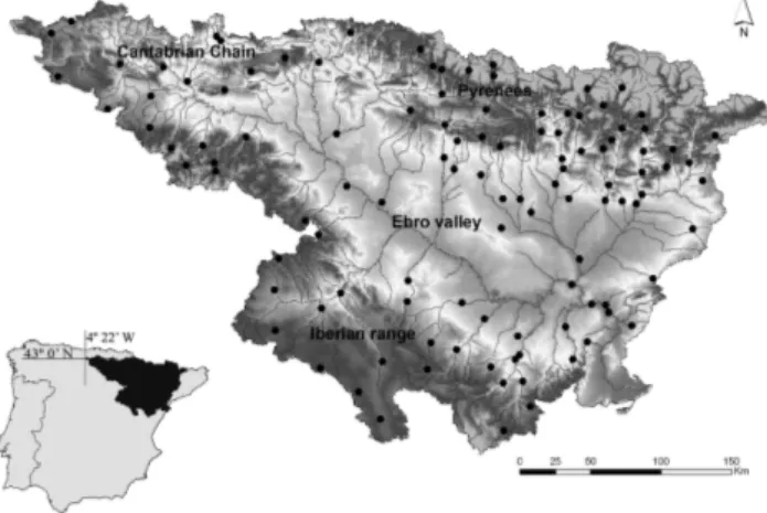
The study area covers the north-east of Spain (Fig. 1). It corresponds to the Ebro Basin, which represents an area of about 85 000 km2. The Ebro valley is an inner depression surrounded by high mountain ranges. It is limited to the North by the Cantabrian Range and the Pyrenees, with maxi-mum elevations above 3000 m a.s.l. The Iberian range closes the Ebro valley to the South, with maximum elevations in the range of the 2000–2300 m. To the East, parallel to the Mediterranean coast, the Catalan Coastal Range closes the Ebro valley, with maximum elevations between 1000 and 1200 m a.s.l.
The climate is influenced by the Cantabric and Mediter-ranean Seas and the effect of the relief on precipitation and temperature. The border mountain ranges isolate the central valley blocking the maritime influence, resulting in a continental climate which experiments aridity conditions (Cuadrat, 1991; Lana and Burgue˜no, 1998; Creus 2001; Vicente-Serrano 2005). A climatic gradient in the NW-SE direction is remarkable, determined by the strong Atlantic in-fluences in the north and north-west of the area during large part of the year and the Mediterranean influence to the east. Mountain ranges add complexity to the climate of the region. The Pyrenees extend the Atlantic influence to the east by in-creasing precipitation, whereas the Cantabrian Range, which runs parallel to the Atlantic coastland in the NW, is a bar-rier to the humid flows and has a noticeable climate contrast between the north (humid) and the south (dry) slopes.
Fig. 1.Location of the study area and the observatories used on this study.
Close to the Mediterranean Sea the precipitation amount also increases as a consequence of the maritime influence. Nevertheless, the precipitation frequency, intensity and sea-sonality are very different compared to the areas in the North, where precipitation is frequent but rarely very intense, with the exception of mountainous areas (Garc´ıa-Ruiz et al., 2000). The most extreme precipitation events are recorded along the Mediterranean seaside (Llasat, 2001; Romero et al., 1998; Pe˜narrocha et al., 2002). The Ebro Basin has a long record of social, economic and environmental damages caused by extreme rainfall events (Garc´ıa-Ruiz et al., 2000; Lasanta, 2003) due to its complex climatology, as a meteoro-logical border region, and the contrasted relief.
2.2 Data base
The database consisted on 112 selected rainfall series from the Ebro Hydrographical Confederation SAIH system – Au-tomatic Hydrological Information Network (Fig. 1). Each station provides precipitation data at a time resolution of 15 min. The system started in 1997, and is the only dense net-work providing sub-daily resolution data in the region. We used all available series data for the period 1 January 1997 to 31 December 2006.
The rainfall series were subjected to a quality control that allowed identifying wrong records due to system failures. These records were replaced by the corresponding ones from a nearby station. This allowed creating an erosive events database (EEDB). The erosive events were determined by the RUSLE criterion: an event is considered erosive if at least one of this conditions is true: i) the cumulative rain-fall is greater than 12.7 mm, or ii) the cumulative rainrain-fall has at least one peak greater than 6.35 mm in 15 min. Two con-secutive events are considered different from each other if the cumulative rainfall in a period of 6 h is greater than 1.27 mm.
2.3 Rainfall erosivity index
The rainfall erosivity indices employed were the average EI30 index events and the RUSLE R factor. These indices have been widely used, making it possible to compare the re-sults with those of other studies. The RUSLE model uses the Brown and Foster (1987) approach for calculating the aver-age annual rainfall erosivity,R(MJ mm ha−1h−1y−1):
R= 1
n
n X
j=1 mj
X
k=1
(EI30)k (1)
wherenis the number of years of records,mj is the number of erosive events of a given yearj, and EI30 is the rainfall erosivity index of a singular eventk. Thus, the R factor is the average value of the annual cumulative EI30over a given period. The event’s rainfall erosivity EI30(MJ mm ha−1h−1) is obtained as follows:
EI=EI30= o X
r=1
ervr !
I30 (2)
where er and vr are, respectively, the unit rainfall energy (MJ ha−1mm−1) and the rainfall volume (mm) during a time period r, andI30 is the maximum rainfall intensity during a period of 30 min in the event (mm h−1). The unit rainfall energy,er, is calculated for each time interval as:
er =0.29[1−0.72 exp(−0.05ir)] (3) where ir is the rainfall intensity during the time interval (mm h−1). In addition to the R factor, we also calculated the average EI30of the erosive events over the study period.
The average EI30, is calculated as the mean erosivity of all rainfall events. Since the frequency distribution of EI30 is highly skewed (it follows a logarithmic law), the average EI30is in fact most correlated with the highest erosive events. Maps showing the spatial distribution of the average EI30 in-dex complement the information given by the R factor alone. 2.4 Spatial modelling
In many studies the rainfall erosivity calculation is reduced to at-site analysis. An improvement focus on the reduction of the risk of erosion in landscape management and conserva-tion planning is to obtain continuous maps for large areas as a preliminary step to evaluate the hazard. For this purpose a common procedure is the mapping of at-site estimated rain-fall erosivity index values by means of interpolation tech-niques (e.g., Prudhome and Reed, 1999; Weisse and Bois, 2002).
For the regression-based models, a digital elevation model (DEM) and a digital coverage of the Iberian Peninsula coast-line were used. Both were obtained from the Ebro Hydro-graphical Confederation (http://www.chebro.es/).
2.4.1 Global methods
The global method used was generalized least squares (GLS) multiple regression. Regression is a global approach to spa-tial interpolation, and it is based on finding empirical rela-tionships between the variable of interest and other spatial variables. Regression-based techniques adapt to almost any space and usually generate adequate maps (Goodale et al., 1998; Vogt et al., 1997; Ninyerola et al., 2000). The relation-ships between climatic data and topographic and geographic variables have been extensively analyzed throughout the sci-entific literature, and regression-based models allow exploit-ing this relationship to produce maps of the climatic param-eters. Some authors have shown the advantages of incorpo-rating the information provided by ancillary data on mapping extreme rainfall probabilities (Beguer´ıa and Vicente-Serrano, 2006; Casas et al., 2007). Regression methods can be es-pecially adequate in large regions with complex atmospheric influences, such as the Ebro Valley (Daly et al., 2002; Weisse and Bois, 2002; Vicente-Serrano et al., 2003), or if the sam-ple network is not dense enough for local interpolation meth-ods (Dirks et al., 1998).
GLS is an extension of the most common ordinary least squares (OLS) regression, which allows for autocorrelation in the dependent variable (Cressie, 1993). When dealing with spatial variables, it is common assumption that the observa-tions are autocorrelated; this property forms, in fact, the ba-sis of all geostatistical and mixed methods. The existence of autocorrelation in the residuals violates one of the main assumptions of OLS, thus making this technique not suit-able for climatic varisuit-ables with geographical imprint. This problem can be easily solved by using alternative regression techniques that account explicitly for spatial autocorrelation, such as GLS (Beguer´ıa and Pueyo, 2009). The differences between both methods can be easily explained by introduc-ing their mathematical background. From the common OLS formula:
y=Xβ+ε (4)
wherey is the dependent variable,Xis a matrix ofp inde-pendent variables (model matrix),βis a vector ofp+1 model coefficients to estimate, including a constantβ0, andε is a vector of random errors. In OLS it is assumed that the er-rors are normally distributed with mean 0 and variance I:
ε∼N 0, σ2I
. In GLS, on the contrary, it is generally as-sumed thatε∼N (0, 6), where the error variance-covariance matrix6is symmetric and positive-definite. Different diag-onal entries in6correspond to non-constant error variances, while nonzero off-diagonal entries correspond to correlated errors. Since the error variance-covariance matrix6 is not
known, it must be estimated from the data along with the re-gression coefficientsβ. Due to the high number of elements of6, it needs to be approximated by a parametric model. In the case of spatial regression, 6 can be adequately param-eterized by a semi-variogram model. The semi-variogram model explains the covariance between the errors based on the distance between pairwise observations. Since the semi-variogram constitutes the basis of geostatistical interpolation methods, it is explained in depth in a further section (see Sect. 2.4.3).
We used a set of independent variables at a spatial reso-lution of 100 m. Elevation is usually the main determinant of the spatial distribution of climatic variables. Neverthe-less, other variables such as the latitude and longitude, or the incoming solar radiation may also have an influence on the distribution of erosive rains. All variables were derived from a DEM (UTM-30N coordinates). The incoming solar radia-tion is a spatially continuous variable that depends on the ter-rain aspect (northern and southern slopes have low and high incoming solar radiation values, respectively). The annual mean incoming solar radiation was calculated following the algorithm of Pons and Ninyerola (2008). All these variables were processed in the MiraMon GIS package (Pons, 2006). Low-pass filters with radii of 5, 10 and 25 km were applied to elevation, slope and incoming solar radiation in order to measure the widest influence of these variables.
We used a Gaussian semivariogram model to parameter-ize the spatial autocorrelation between regression errors. As independent variables we used the spatial coordinates (longi-tude and lati(longi-tude) in km and their squares (km2), the eleva-tion (m a.s.l.), and the incoming solar radiaeleva-tion (J d−1). The R statistical analysis package (R Development Core Team, 2008) was used for the regression analysis.
2.4.2 Local methods
In global methods, local variations are dismissed as ran-dom, unstructured noise, and the climatic map is created on the basis of general structure of the variable at all avail-able points (Borrough and McDonnell, 1998). Local meth-ods, on the contrary, use only the data of the nearest sam-pling points for climatic mapping. Since interpolated values at ungauged locations depend on the observed values, local methods strongly depend on a sufficiently dense and evenly spaced sampling network.
Two local methods were used: inverse distance weight-ing (IDW) and splines. The IDW interpolation is based on the assumption that the climatic value at an unsampled point
factor:
z (x)= n P i=1
z (xi) dij−r n P i=1
dij−r
(5)
wherez(x)is the predicted value,z(xi)is the climatic value at a neighbouring weather station,dij is the distance between
z(x)andz(xi), andris an empirical parameter. Models with
r=1,r=2 andr=3 were tested.
The splines method is based on a family of continuous, regular and derivable functions. Splines are similar to the equations obtained from the trend surfaces or regression-based methods, but they are fitted locally from the neighbour-ing points around the candidate locationx. A new function is created for each locationx, without lost of continuity proper-ties among the curves. Smoothing or tension parameters can be specified, resulting in more or less smoothed maps. The predicted valuez(x)is determined by two terms:
z(x)=T (x)+ n X
i=1
λjψj(ri) (6) whereT (x)is a polynomial smoothing term, and the second term groups a series of radial functions where ψj(ri)is a known group of functions, andλj represents the parameters (Mitasova et al., 1995):
ψ (ri)= − h
lnϕri 2
+Ei
ϕri 2
+CE
i
(7) whereφ is the tension coefficient, CE=0.577215. . . is the Euler constant,Ei is the exponential integral function, andri is:
ri = q
(x−xi)2+(y−yi)2 (8) The algorithms for fitting splines are quite complex but are currently standard in GIS packages. In this paper several spline interpolations were used as implemented in the Ar-cGIS 9.3 software. Tension and smoothing parameters were
φ=400,φ=5000,T (x)=0 andT (x)=400. 2.4.3 Geostatistical interpolation methods
Kriging methods assume that the spatial variation of a con-tinuous climatic variable is too irregular to be modelled by a continuous mathematical function, and its spatial variation could be better predicted by a probabilistic surface. This tinuous variable is called a regionalized variable, which con-sists of a drift component and a random, spatially correlated component (Burrough and McDonnell, 1998). Hence, the spatially located climatic variablez(x)is expressed by:
z(x)=m(x)+ε′(x)+ε′′ (9) wherem(x)is the drift component, i.e. the structural varia-tion of the climatic variable,ε′(x) are the spatially correlated
residuals, i.e. the difference between the drift component and the sampling data values, and ε′′ are spatially independent residuals. The predictions of kriging-based methods are cur-rently a weighted average of the data available at neighbour-ing samplneighbour-ing points (weather stations). The weightneighbour-ing is cho-sen so that the calculation is not biased and the variance is minimal. A function that relates the spatial variance of the variable is determined using a semi-variogram model which indicates the semivariance (γ) between the climatic values at different spatial distances.
The semivariogram describes the way in which similar ob-servation values are clustered in space, in accordance with Tobler’s first law of geography (Tobler, 1970). The semivari-ogram is therefore a measure of the dissimilarity of data pairs as the spatial separation between them increases (Deutsch and Journel, 1998). The semivariance is calculated for lagged sets of separation vectorshuas half the mean squared pairwise difference between the N observed values within the spatial lag,u:
γu(hu)= 1 2N (hu)
X
N (hu)
[z (u)−z (u+hu)]2 (10)
To summarize the autocorrelation in space, a product-sum covariance model was automatically fitted to the semivari-ogram. First, only the sample semivariograms,γs,t(hs,0), were considered. Valid semivariogram models were fitted to them, estimating automatically the partial range (φu) and sill (sillu) and adding a nugget discontinuity (τu) at the ori-gin to reflect spatial uncertainty if required. Semivariogram models must be selected from a set of allowable functions that are conditionally negative definite (Mcbratney and Web-ster, 1986), i.e. spherical, exponential or gaussian models (Deutsch and Journel, 1998). There is some argument over the correct way to proceed in semivariogram model fitting (Diggle et al., 2002; Goovaerts, 1997); we favoured auto-matically fitting by the OLS method, followed by adjustment by eye, to reduce the effect of outliers. The Gaussian func-tion adjusted best. Predicfunc-tions may improve depending in the number of neighbours included in the interpolation. Our data were not very sensible to the number of neighbours. A combination of 9 neighbours, including at least 3 fitted best.
Several types of kriging methods have been proposed, de-pending on how the drift componentm(x)is modelled (see, e.g., the reviews by Isaaks and Strivastava, 1989; Goovaerts, 1997; Burrough and McDonnell, 1998). Simple kriging (SK) assumes a known constant trend (expected value), m(x)=0, and relies on a covariance function. However, neither the ex-pectation nor the covariance function are usually known, so simple kriging is seldom used. In ordinary kriging (OK), the most common type of kriging, an unknown constant trend is assumed,m(x)=E(z(x)), and the estimation relies on a semivariogram model which is estimated from the sample.
in space. This is often not the case with climatic variables, which tend to show spatial trends due to differences in the exposure to the atmospheric factors. Universal kriging (UK) allows incorporating non-stationarity by assuming a general linear trend model,
m(x)= p X
k=0
βkf (x) (11)
wherep defines the order of the polinomial model on the spatial coordinates of the point,f (x). This process is often called trend removal, and it is interesting because it can cap-ture a real spatial struccap-ture present in the data. However, it in-creases the complexity of the kriging model by adding more parameters for estimation. A two-dimensional quadratic sur-face, for example, adds five parameters beyond the intercept parameter that need to be estimated. As it is well known, the more parameters to be estimated, the more uncertain the model becomes.
Spatial structure can also arise in climatic data due to co-variation with other geographical factors such as the eleva-tion or the solar incoming radiaeleva-tion. Co-kriging (CK) allows considering the influence of external variables (co-variates) by analysing the cross-correlation between the errors of the different variables,ε′
1(x),ε′2(x), etc.
Spatial correlation may occur at different distances when different directions are considered; this characteristic is calledanisotropy. Since the Ebro basin has a marked NW-SE structure, the effect of including anisotropy in the model was also evaluated.
In our study we compared OK, UK and CK methods. The order of the trend removal component in UK was determined by the lowest root mean square error, computed by a leave-one-out bootstrap process. In the case of CK we used the elevation, as determined by a digital terrain model (DTM), as the spatially distributed co-variate; the kriging method used was the best one from the previous methods, i.e. OK and UK. All geostatistical analyses were done with the ArcGIS 9.3 software.
2.4.4 Mixed methods
Mixed methods, also called “hybrid” (Hengl et al., 2004), are based on a combination of regression and local interpolation techniques or kriging, exploiting the ability of regression to relate the target variable to other spatially distributed vari-ables and the spatial self-correlation acting at the local scale on most spatial variables. Alternative forms of mixed meth-ods have been proposed in the last years for mapping en-vironmental variables (Odeh et al., 1994, 1995; Brown and Comrie, 2002; McBratney et al., 2003; Hengl et al., 2004; Ninyerola et al., 2007; Vicente-Serrano et al., 2007). These and other studies have demonstrated that mixed methods usu-ally allow for more precise and detailed representations of the target variables.
There are several types of mixed interpolation methods which vary upon their procedure. When regression residuals (ε) are interpolated by means of kriging two methods can be used: i) in kriging with external drift (KED), the drift com-ponent is defined by regression upon some auxiliary vari-ables and fitted together with the spatial distribution of the residuals (Wackernagel, 1998; Chiles and Delfiner, 1999); ii) in regresion-kriging (RK) the drift and the residuals are fit-ted separately and then summed (Ahmed and Marsily, 1987; Odeh et al., 1994, 1995). Other kind of mixed methods in-terpolate residuals using local methods as the inverse dis-tance weighting interpolation or splines (Vicente-Serrano et al., 2003; Ninyerola et al., 2007).
In this study we used RK. To avoid misconceptions or sub-optimal solutions (Hengl et al., 2004), regression predic-tions were calculated by means of GLS (see Sect. 2.4.1.), and then residuals surfaces were fitted by OK and added to the GLS predictions. The R statistical analysis package (R De-velopment Core Team, 2008) was used for RK.
2.5 Local uncertainty assessment
Spatial modelling involves uncertainty associated to the con-tinuous estimated surface. Estimating the standard error of the predictions is necessary for completing the spatial mod-elling. In the case of spatial variables the problem is more complex, since the standard error of the predictions is also a spatial variable (Goovaerts, 2001). In this study we have used the technique called Gaussian geostatistical simulation (GGS). GSS generates multiple, equally probable represen-tations of the spatial distribution of the attribute under study. A normal score transformation is performed on the data so that it will follow a standard normal distribution (mean=0 andσ2=1). Conditional simulations are then run on this nor-mally distributed data, and the results are back-transformed to obtain simulated output in the original units. Given a high enough number of simulations, its average will tend to equal the surface estimated by SK. The standard deviation of the simulations is taken as an estimator of the standard error of the estimated surface, from which confidence bands can be constructed. These representations provide a way to measure uncertainty for the unsampled locations taken all together in space rather than one by one (as measured by the kriging variance). We performed a series of 1000 conditioned sim-ulations from an initial SK model with second order trend removal. GGS was performed with the ArcGIS 9.3 software. 2.6 Validation statistics
Table 1. Computation of several goodness of fit statistics used on this study.
Statistical critera Definitions:
N: no. of observations O: observed value O: mean of obs. values P: predicted value Pi′=Pi−O Oi′=Oi−O
Mean bias error (MBE) MBE=N−1 N P i=1
(Pi−Oi)
Mean absolute error (MAE) MAE=N−1 N P i=1
|Pi−Oi|
Willmontt’sD D=1−
N
P
i=1
(Pi−Oi)2 N
P
i=1 Pi′
+
Oi′
2
and the observed values. Cross-validation techniques are pre-ferred to more traditional split-sample procedures for esti-mating generalization error, since they allow an independent validation without sacrificing an important amount of data (Weiss and Kulikowski, 1991). Cross-validation is compul-sory when comparing exact interpolators such as IDW or splines, which by definition give an exact value at the lo-cations used for fitting the model, i.e. all residuals at these points are zero.
We used a set of goodness of fit statistics not to rely on a single one (Table 1). These include: i) the mean bias er-ror (MBE), which is centred around zero and is an indica-tor of prediction bias; ii) the mean absolute error (MAE), which is a measure of the average error; and iii) the agree-ment indexD(Willmott, 1981), which scales the magnitude of the variables, retains mean information and does not am-plify the outliers. We avoided using the root mean square error (RMSE) because it is highly biased by outlier obser-vations, and also because it is difficult to discern whether it reflects the average error or the variability of the squared er-rors (Willmott and Matsuura, 2005).
3 Results
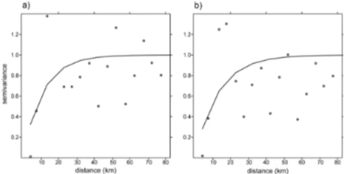
The spatial structure of the data was initially assessed by em-pirical semivariograms, (Fig. 2). Spatial autocorrelation was present for both variables at relatively short distances (less than 15 km). Above this distance the spatial autocorrelation disappeared, as it was also visible in the fitted Gaussian semi-variogram models.
All interpolation methods were able to capture the re-gional distribution of the two rainfall erosivity
parame-Fig. 2.Empirical semivariograms (circles) and fitted semivariogram Gaussian models (lines) of the rainfall erosivity indices:(A)R fac-tor;(B)EI30index. Range parameters are: 10.98 km (R factor) and
13.05 km (EI30index).
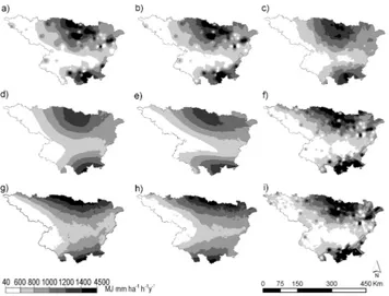
ters (Figs. 3 and 4). Differences between interpolation methods were more evident for the EI30 index than for the R factor. The R factor was highest – from 1200 to 4500 MJ mm ha−1h−1y−1 – in two areas: i) in the Pyre-nees Range at the north, especially in the central part; and ii) in the south-east mountainous part, corresponding to the Iberian Range and the southern east region. The lowest val-ues – from 40 to 800 MJ mm ha−1h−1y−1 – appeared in the north-west of the area and in the centre of the Ebro River valley. The spatial distribution of the EI30index was slightly different, showing a gradient from the north-west (Cantabric Sea) to the south-east (Mediterranean Sea), mod-ified to a certain extent by the relief. The highest values – from 70 to 190 MJ mm ha−1h−1– were found in the south-east corner, along the coast. Lower values – from 8 to 40 MJ mm ha−1h−1– are found close to the Cantabric Sea. This pattern is similar to the distribution of the extreme rain-fall events in the region (Beguer´ıa et al., 2009), and is an indicator of the EI30index being closely related to the most intense rainfall events.
3.1 Spatial distribution of the rainfall erosivity indices
The spatial distribution of both indices over the study area can be explained to a large extent by the proximity to – or iso-lation from – the water masses (the Cantabrian and Mediter-ranean seas). The relief, with mountain ranges to the north, south and east of the region, modify this general pattern by increasing rainfall in those areas. Another effect of the relief is the isolation of the central area from the main precipitation sources, i.e. creating a zone of rain shadow.
Fig. 3. Rainfall erosivity maps (RUSLE R factor) for the Ebro Basin: (a)inverse distance weighting surface;(b)spline with ten-sion (φ=5000);(c)smoothing spline (φ=400);(d)ordinary kriging; (e)ordinary kriging with anisotropy;(f)universal kriging;(g) co-kriging;(h)regression model (GLS);(i)regression-kriging.
methods varied slightly depending on the value of the r and
ψparameters (maps not shown), but in all cases they had this characteristic. The smoothed splines method, which includes a smoothing function to reduce excessive influence of local observations, produced a more regularized output.
Geostatistical methods – OK, OK with anisotropy and CK – produced much more smoothed results than the local meth-ods, yet retaining a good degree of detail. Anisotropy mod-ified only slightly the results from OK by orienting the es-timated surface in the direction NW-SE. The R factor map resulting from UK – detrending the data by a second order polynomial – was very similar to the surfaces generated by local interpolators, i.e. it showed a high influence of local ob-servations. The result of CK – OK with elevation as a covari-ate – showed only a marginal increase in detail with respect to OK.
The surface generated by GLS regression was similar to the CK surface. The regression models were significant at
α=0.05, although the coefficient of determination (r2) of the models was not high (0.212 for the R factor and 0.218 for the EI30 index). The only significant variables atα=0.05 were the spatial coordinates, and just for the R factor, revealing the poor explanatory capacity of other auxiliary variables – elevation and solar radiation (Table 2). This was also evi-dent by the low values of the beta coefficients of these two variables.
In the maps obtained by regression-kriging (RK) the influ-ence of the interpolation of the residuals was evident. The predicted map was very similar to the UK surface, especially in the case of the R factor. In the EI30 index maps the influ-ence of elevation and radiation could be eye noticed.
Fig. 4. Rainfall erosivity maps (average EI30index of the erosive
events) for the Ebro Basin:(a)inverse distance weighting surface; (b)spline with tension (φ=5000);(c)smoothing spline (φ=400);(d) ordinary kriging;(e)ordinary kriging with anisotropy;(f)universal kriging;(g)co-kriging;(h)regression model (GLS);(i)regression kriging.
Table 2. Results of the generalized least squares regression of the R factor and the EI30 index: regression coefficients, standardized coefficients and significance level for each independent variable.
Variable Beta Standardized Significance coeff. beta coeff. level
R factor
longitude 14.411 2.658 0.023∗ longitude2 −21.803 −2.582 0.219 latitude −0.010 −2.380 0.041∗ latitude2 0.003 2.744 0.191 elevation 0.087 0.047 0.579 solar radiation −201.853 −0.031 0.732
EI30index
longitude 0.255 1.132 0.304 longitude2 −0.849 −2.418 0.239 latitude −0.0001 −0.861 0.432 latitude2 0.0001 2.166 0.291 elevation 0.003 0.045 0.593 solar radiation 0.691 0.003 0.977
∗variable is significant at confidence levelα=0.05.
3.2 Validation
Table 3. Accuracy measurements for the R factor models: mean and standard deviation of the observed and predicted values, and cross-validations statistics.
Validation statistics
Mean Standard MBE MAE Willmott’s
deviation D
Observed 891.40 621.77
Predicted
Inverse Distance Weighting (r=1) 896.64 292.49 5.24 355.26 0.534 Inverse Distance Weighting (r=2) 891.75 346.59 0.350 356.33 0.577 Inverse Distance Weighting (r=3) 896.85 420.40 5.44 367.40 0.595 Smoothed splines [T (x, y)=400] 895.86 275.70 4.45 354.99 0.521 Splines with tension (φ=400) 896.74 268.30 5.33 357.45 0.497 Splines with tension (φ=5000) 890.21 324.54 −1.19 348.27 0.573 Ordinary kriging (OK) 885.37 252.11 −6.03 357.76 0.491 Ordinary kriging with anisotropy 890.06 244.41 −1.34 356.45 0.491 Universal kriging (UK) 890.60 359.08 −0.806 355.79 0.584 Co-kriging (OK + elev) 877.69 318.02 −13.71 369.52 0.513
Regression (GLS) 900.53 292.64 9.13 386.31 0.468
Regression-Kriging 910.60 292.02 19.20 385.16 0.480
(GLS + residuals kriging)
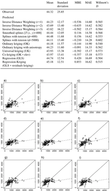
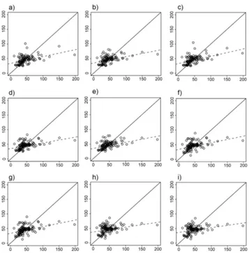
40–4500 MJ mm ha−1h−1y−1, and 23.8 for EI30, which varied in the range 8–190 MJ mm ha−1h−1. Compared with that, the standard deviation of the estimations ranged be-tween 244.4 and 420.4 forR and 11.6 and 16.2 for EI30. Consequently, all models had relatively large absolute er-rors, which were higher than 30% of the mean predicted value for most of them. Similarly, the values of the Will-mott’s D statistic were low. These facts reflect the high random character of both rainfall erosivity indices. The low performance of the models was mostly due to their in-ability to predict the highest values, especially those above 2000 MJ mm ha−1h−1y−1 for R and 100 MJ mm ha−1h−1 for EI30, respectively. This can be clearly seen in the good-ness of fit plots (Figs. 5 and 6).
Differences between the models regarding the validation statistics were narrow, but allowed for a comparison. Ac-cording to the validation statistics the local methods ranked best for both indices, showing highest Willmott’s D val-ues, and lowest MBE and MAE. The R factor was best predicted by inverse distance weighting withr=3, followed by universal kriging, whereas the EI30 index was best fit-ted by splines with tension (φ=5000), followed by IDW withr=3. Geostatistical models yielded good results, es-pecially Universal Kriging, equalled by Co-kriging (OK plus elevation) in the case of the EI30 index. The result of including anisotropy in OK was only marginally better. Finally, regression based methods – GLS and RK – yielded the lowest validation statistics.
3.2.1 Local uncertainty
The previous results evidenced the high level of uncertainty of the predictions of both erosivity indices. The uncertainty model, however, is also a spatial variable and can have strong differences between regions in the study area. The results of Gaussian geostatistical simulation (GGS) helped assessing spatial differences in the uncertainty model (Fig. 7). From
Table 4.Accuracy measurements for the EI30index models: mean
and standard deviation of the observed and predicted values, and cross-validations statistics.
Validation statistics
Mean Standard MBE MAE Willmott’s
deviation D
Observed 44.32 25.85
Predicted
Inverse Distance Weighting (r=1) 44.23 12.17 −0.536 14.60 0.565 Inverse Distance Weighting (r=2) 43.69 13.40 −0.635 14.62 0.582 Inverse Distance Weighting (r=3) 43.82 16.22 −0.502 15.17 0.584 Smoothed splines [T (x, y)=400] 44.44 12.05 0.116 14.58 0.568 Splines with tension (φ=400) 44.48 11.68 0.156 14.62 0.553 Splines with tension (φ=5000) 44.11 13.40 −0.210 14.28 0.602 Ordinary kriging (OK) 44.18 11.57 −0.144 14.90 0.540 Ordinary kriging with anisotropy 44.23 11.60 −0.091 14.33 0.562 Universal kriging (UK) 43.93 13.38 −0.392 15.17 0.573 Co-kriging (OK + elev) 43.97 13.41 −0.357 15.18 0.573
Regression (GLS) 44.74 12.54 0.420 16.69 0.504
Regression-Kriging 45.18 12.51 0.853 16.62 0.515
(GLS + residuals kriging)
Fig. 5.Comparison between observed (ordinate axis) and predicted (abscissa axis) values for the interpolation methods used for the spa-tial distribution of the R factor, line of perfect fit (continuous) and regression line (dashed). (a)inverse distance weighting (r=2);(b) smoothing spline (φ=400);(c)splines with tension (φ=5000);(d) ordinary kriging;(e)ordinary kriging with anisotropy;(f)universal kriging;(g)co-kriging;(h)regression model (GLS);(i) regression-kriging.
Fig. 6. Comparison between observed (ordinate axis) and pre-dicted (abscissa axis) values for the different interpolation meth-ods used for the spatial distribution of the EI30index, line of
per-fect fit (continuous) and regression line (dashed). (a)inverse dis-tance weighting (r=2);(b)smoothing spline (φ=400);(c)splines with tension (φ=5000);(d)ordinary kriging;(e)ordinary kriging with anisotropy;(f)universal kriging;(g)co-kriging;(h)regression model (GLS);(i)regression-kriging.
the magnitude of the error ranged between 10 and 100% of the mean value. The standard error increased rapidly for re-gions located more than∼15 km away from any observatory, indicating that the range of the spatial influence of the ob-servations was quite small. This was already suggested by the preliminary analysis of the semivariogram. From that distance, which was larger for the EI30 index than for the R factor, uncertainty distributed randomly.
4 Discussion and conclusions
Rainfall erosivity is an indicator of the precipitation ag-gressiveness, and depends on the rainfall energy (raindrop size distribution and kinetic energy) and the intensity of the storm event. Rainfall under Mediterranean climate is char-acterized by high temporal variability and a flashy character. This last characteristic affects especially the rainfall erosiv-ity, which depends on the occurrence of few, very intense, events (Gonz´alez-Hidalgo et al., 2007).
In this study we used the RUSLE R factor and the average EI30index of the erosive events to assess the spatial distribu-tion of rainfall erosivity on the northeast sector of the Iberian Peninsula. Both variables are characterized by a high tem-poral variability, especially in the Mediterranean area and
Fig. 7. Local uncertainty modeled by Gaussian geostatistical sim-ulation (GGS) for the R factor and the EI30 index: (a)mean of
R factor;(b)mean of EI30index;(c)standard error of R factor;(d) standard error of EI30index.
in geographically complex regions (Leek and Olsen, 2000; Gonz´alez-Hidalgo et al., 2007). During the initial stage of the analysis it was evident that close observatories could have very different values ofR and EI30, and this was confirmed by the analysis of the semivariogram.
818 MJ mm ha−1h−1y−1 in Central Spain (Boellstorff and Benito, 2005); or 419.01 to 1124.36 MJ mm ha−1h−1y−1in Sicily (Onori et al., 2006). We are not aware of previous stud-ies analyzing the spatial distribution of the average EI30 in-dex.
Despite the high spatial variability of both indices, the mapping methods tested were able to capture the main spa-tial pattern of rainfall erosivity in the area. The spatial distribution can be explained by seasonal atmospheric be-haviour which causes the major stormy events. In the Pyre-nees these events are related with south-western flows con-fronting the mountains triggering orographic rainfall in win-ter, and convective storms in summer. Close to the Mediter-ranean Sea the heating contrast between the atmosphere up-per levels and continental and maritime surfaces, more in-tense during fall, generates inin-tense storms. This is the prin-cipal cause of heavy rainfalls in the southeastern area (Llasat and Puigcerver, 1997). These synoptic situations explain the spatial pattern of rainfall erosivity, which is linked to the most extreme events of the year. In addition, the strong re-lief adds complexity to the climate dynamics making more complex to obtain reliable models. It is responsible of oro-graphic precipitation increase, and it also generates temper-ature differences in narrow spaces which contribute to the formation of convective cellules and local storms. Thus, the general pattern present in all rainfall erosivity maps show a clear north-west to south-east gradient, and marked local dif-ferences caused by the relief.
The comparison of several interpolation techniques yielded mixed results, since no single method arouse as op-timal according to all validation metrics, and the differences between models were narrow. Local interpolation methods yielded the best results overall, which can be explained by the very high spatial variability of rainfall erosivity as found in the preliminary semivariogram analysis. However, the maps produced by these methods masked the global pat-tern by introducing spatial noise due to the excessive weight given to local observations. Geostatistical methods were able to capture more general pattern ranking slightly lower from the local methods in the validation statistics. Among them, universal kriging (UK) ranked best and was able to cap-ture local detail whereas conserving also the general pattern. Regression-based methods (GLS regression and regression-kriging) ranked lowest due to their most global character. Be-sides, the independent variables selected – elevation and so-lar radiation – did not have significant explanatory capacity. Regression-kriging ranked slightly better than regression-based methods, but their prediction was not better than that of UK.
The results obtained in the present study reflected the highly random character of rainfall erosivity, evaluated by both indices – the R factor and EI30 index. In general, the models were bad at predicting the highest values of both in-dices, due to the presence of outlier observations. The uncer-tainty of the predicted values can be explained by the natural
climate variability in the study area, and also by the length of the analysis period. Other authors have reported high variability of soil erosion values in the Mediterranean re-gion, both in space and time (Gonz´alez-Hidalgo et al., 2007). Though, more information is needed for the assessment of the causal factors responsible of the high uncertainty present in all models. The quantification of uncertainty by means of Gaussian geostatistical simulation (GGS), expressed by stan-dard error surfaces, allowed estimating confidence bands for the prediction surfaces. These cartographies constituted an important result for the applicability of the rainfall erosivity maps.
The results suggest that the database needs to be im-proved both in time (longer high-frequency precipitation se-ries) and space (denser network). With respect to the length of the data series, it is generally accepted that a minimum of 20 years is desirable for rainfall erosivity analysis (Renard and Freimund, 1994; Renard et al., 1997; Curse et al., 2006; Verstraeten et al., 2006). Unfortunately, there are very few data bases of high time resolution rainfall records and a good spatial coverage, as the one used in this work. Longer se-ries are needed for reducing the strong influence of outlier observations. With respect to the spatial distribution of the data sets, the results showed spatial autocorrelation limited to a perimeter of∼15 km. This fact evidenced the need for improving the spatial coverage if better predictions are to be achieved.
The availability of high-quality environmental maps is a key issue for agricultural and hydrological management in many regions of the World. Rainfall erosivity maps can be of high relevance as a guidance for soil conservation practices, and also because they are usually part of erosion models such as the RUSLE. Recently, the RUSLE model has been imple-mented into GIS packages, integrating all the factors as dif-ferent layers. Hence, the accuracy of the spatial surface of each factor is propagated to the outputs of the model. Com-pared to other climatic variables, rainfall erosivity is char-acterized by a high spatial and inter-annual variability, what makes mapping more difficult.
Further research may be directed to find reliable erosivity indices which can be computed from daily precipitation data. This would allow using daily precipitation data bases, which are usually longer and have a higher spatial coverage. This would lead to more robust results, and will also make trend analysis possible.
Edited by: A. Bronstert
References
Ahmed, S. and De Marsily, G.: Comparison of geostatistical meth-ods for estimating transmissivity using data on transmissivity and specific capacity, Water Resour. Res., 23, 1717–1737, 1987. Arnoldus, H. M. J.: Methodology used to determine the maximum
potential average annual soil loss due to sheet and rill erosion in Morocco, FAO Soils Bulletin, 34, 39–51, 1977.
Beguer´ıa, S. and Vicente-Serrano, S. M.: Mapping the hazard of extreme rainfall by peaks over threshold extreme value analysis and spatial regression techniques, J. Appl. Meteorol., 45, 108– 124, 2006.
Beguer´ıa, S., Vicente-Serrano, S. M., L´opez-Moreno, J. I., and Garc´ıa-Ruiz, J. M.: Annual and seasonal mapping of peak in-tensity, magnitude and duration of extreme precipitation events across a climatic gradient, North-east Iberian Peninsula, Int. J. Climatol., 29(12), 1759–1779, doi:10.1002/joc.1808, 2009. Beguer´ıa, S. and Pueyo, Y.: A comparison of simultaneous
autore-gressive and generalized least squares models for dealing with spatial autocorrelation, Global Ecol. Biogeogr., 18(3), 273–279, 2009.
Boellstorff, D. and Benito, G.: Impacts of set-aside policy on the risk of soil erosion in central Spain, Agr. Ecosyst. Environ., 107, 231–243, 2005.
Borrough, P. A. and McDonnell, R. A.: Principles of geographical information systems, Oxford University Press, 1998.
Brown, D. P. and Comrie, A. C.: Spatial modelling of winter tem-perature and precipitation in Arizona and New Mexico, USA, Climate Res., 22, 115–128, 2002.
Brown, L. C. and Foster, G. R.: Storm erosivity using idealized intensity distributions, T. ASAE, 30, 379–386, 1987.
Casas, M. C., Herrero, M., Ninyerola, M., Pons, X., Rodr´ıguez, R., Rius, A., and Reda˜no, A.: Analysis and objective mapping of extreme daily rainfall in Catalonia, Int. J. Climatol., 27, 399–409, 2007.
Chiles, J. and Delfiner, P.: Geostatistics: modelling spatial uncer-tainty, Wiley, New York, 1999.
Cressie, N. A. C.: Statistics for spatial data, rev. edn., John Wiley and Sons, 1993.
Creus, J.: Las sequ´ıas en el valle del Ebro, in: Causas y consecuen-cias de las sequ´ıas en Espa˜na, edited by: Gil, A. and Morales, A., Universidad D’Alacant, 231–259, 2001.
Cuadrat, J. M.: Las sequ´ıas en el valle del Ebro. Aspectos clim´aticos y consecuencias econ´omicas, Rev. Real Acad. Ciencias, 85, 537– 545, 1991.
Curse, R., Flanagan, J., Frankenberger, B., Gelder, D., Herzmann, D., James, D., Krajenski, W., Kraszewski, M., Laflen, J., Op-somer, J., and Todey, D.: Daily estimates of rainfall, water runoff and soil erosion in Iowa, J. Soil Water Conserv., 61, 191–199, 2006.
Daly, C., Gibson, W. P., Taylor, G. H., Johnson, G. L., and Pasteris, P.: A knowledge-based approach to the statistical mapping of climate, Climate Res., 22, 99–113, 2002.
Deutsch, C. V. and Journel, A. G.: Gslib: Geostatistical software library and user’s guide, Oxford university press, 1998. Diggle, P. J., Ribero, P. J., an dCristensen, O. F.: An introduction
to model basis geostatistics, in: Spatial statistics and
computa-tional methods. Lecture notes in statistics, edited by: Møller, J., Springer-Verlag, New York, 2002.
Diodato, N.: Estimating RUSLEs rainfall factor in the part of Italy with a Mediterranean rainfall regime, Hydrol. Earth Syst. Sci., 8, 103–107, 2004,
http://www.hydrol-earth-syst-sci.net/8/103/2004/.
Dirks, K. N., Hay, J. E., Stow, C. D., and Harris D.: High-resolution studies of rainfall on Norfolk Island. Part II: Interpolation of rain-fall data, J. Hydrol., 208, 187–193, 1998.
Dom´ınguez-Romero, L., Ayuso Mu˜noz, J. L., and Garc´ıa Mar´ın, A. P.: Annual distribution of rainfall erosivity in western Andalusia, southern Spain, J. Soil Water Conserv., 62, 390–401, 2007. Dunkerley, D.: Rain event properties in nature and in rainfall
sim-ulation experiments: a comparative review with recommenda-tions for increasingly systematic study and reporting, Hydrol. Process., 22(22), 4415–4435, doi:10.1002/hyp.7045, 2008. Efron, B. and Tibshirani, R. J.: Improvements on cross-validation:
the .632+ bootstrap method, J. Am. Stat. Assoc., 92, 548–560, 1997.
Garc´ıa-Ruiz, J. M., Arn´aez, J., White, S. M., Lorente, A., and Be-guer´ıa, S.: Uncertainty assessment in the predition of extreme rainfall events: an example from the Central Spanish Pyrenees, Hydrol. Process., 14, 887–898, 2000.
Garrido, J. and Garc´ıa, J. A.: Periodic signals in Spanish monthly precipitation data, Theor. Appl. Climatol., 45, 97–106, 1992. Gobin, A., Jones, R., Kirkby, M., Campling, P., Govers, G.,
Kos-mas, C., and Gentile, A. R.: Indicators for pan-European assess-ment and monitoring of soil erosion by water, Environ. Sci. Pol-icy, 7, 25–38, 2004.
Gonz´alez-Hidalgo, J. C., Pe˜na-Monn`e, J. L., and de Luis, M.: A review of daily soil erosion in western Mediterranean areas, Catena, 71, 193–199, 2007.
Goodale, C. L., Aber, J. D., and Ollinger, S. V.: Mapping monthly precipitation, temperature and solar radiation from Ireland with polynomial regression and a digital elevation model, Climate Res., 10, 35–49, 1998.
Goovaerts, P.: Geostatistics for natural resources evaluation, Oxford University Press, New York, 1997.
Goovaerts, P.: Using elevation to aid the geostatistical mapping of rainfall erosivity, Catena, 34, 227–242, 1999.
Goovaerts, P.: Geostatistical modelling of uncertainty in soil sci-ence, Geoderma, 103, 3–26, 2001.
Hengl, T., Heuvelink, G. B. M., and Stain, A.: A gereric frame-work for spatial prediction of soil variables based on regression-kriging, Geoderma, 120, 75–93, 2004.
Hoyos, N., Waylen, P. R., and Jaramillo, A.: Seasonal and spatial patterns of erosivity in a tropical watershed of the Colombian Andes, J. Hydrol., 314, 177–191, 2005.
Hudson, N.: Soil Conservation, Cornell University Press, Ithaca, 1971.
Kinnell, P. I. A. and Risse, L. M.: USLE-M: Empirical modelling rainfall erosion through runoff and sediment concentration, Soil Sci. Soc. Am. J., 62, 1667–1672, 1998.
ICONA: Agresividad de la lluvia en Espa˜na. Valores del factor R de la Ecuaci´on Universal de P´erdida de Suelo, Ministerio de Agri-cultura, pesca y alimentaci´on, Espa˜na, 1988.
Isaaks, E. H. and Strivastava, R. M.: An introduction to applied geostatistics, Oxford University Press, Oxford, 1989.
rainfall characteristics, Geoderma, 16, 389–401, 1976.
Lana, X. and Burgue˜no, A.: Spatial and temporal characterization of annual extreme droughts in catalonia (Northeast Spain), Int. J. Climatol., 18, 93–110, 1998.
Lasanta, T.: Gesti´on agr´ıcola y erosi´on del suelo en la cuenca del Ebro: el estado de la cuesti´on, Zub´ıa, 21, 76–96, 2003.
Llasat, M. C. and Puigcerver, M.: Meteorological factors associated with floods in the north-eastern part of the Iberian Peninsula, Nat. Hazards, 5, 133–151, 1994.
Llasat, M. C.: An objective classification of rainfall events on the basis of their convective features: Application to rainfall inten-sity in the northeast of Spain, Int. J. Climatol., 21, 1385–1400, 2001.
Leek, R. and Olsen, P.: Modelling climatic erosivity as a factor for soil erosion in Denmark: changes and temporal trends, Soil Use Manage., 16, 61–65, 2000.
Lim, K. J., Sagong, M., Engel, B. A., Tang, Z., Choi, J., and Kim, K.: GIS-based sediment assessment tool, Catena, 64, 61–80, 2005.
L´opez-Vicente, M., Navas, A., and Mach´ın, J.: Identifying erosive periods by using RUSLE factors in mountain fields of the Central Spanish Pyrenees, Hydrol. Earth Syst. Sci., 12, 523–535, 2008, http://www.hydrol-earth-syst-sci.net/12/523/2008/.
Mart´ın-Vide, J.: Diez caracter´ısticas de la pluviometr´ıa espa˜nola decisivas en el control de la demanda y el uso del agua, Bolet´ın de la AGE, 18, 9–16, 1994.
McBratney, A. B. and Webster, R.: Chosing functions for semi-variograms of soil properties and fitting them to sampling esti-mates, J. Soil Sci., 37(4), 617–639, 1986.
McBratney, A., Mendoc¸a-Santos, M., and Minasny, B.: On digital soil mapping, Geoderma, 117, 3–52, 2003.
Millward, A. A. and Mersey, J. E.: Adapting the RUSLE to model soil erosion potential in a mountainous tropical watershed, Catena, 38, 109–129, 1999.
Mitasova, H., Mitas, L., Brown, W. M., Gerdes, D. P., Kosinovsky, I., and Baker, T.: Modelling spatially and temporally distributed phenomena: new methods and tools for GRASS GIS, Int. J. Ge-ogr. Inf. Syst., 9, 433–446, 1995.
Mutua, B. M., Klik, A., and Loiskandl, W.: Modeling soil erosion and sediment yield at a catchment scale: the case of masinga catchment, Kenya, Land Degrad. Dev., 17, 557–570, 2006. Ninyerola, M., Pons, X., and Roure, J. M.: A methodological
ap-proach of climatological modelling of air temperature and pre-cipitation through GIS techniques, Int. J. Climatol., 20, 1823– 1841, 2000.
Ninyerola, M., Pons, X., and Roure, J. M.: Monthly precipitation mapping of the Iberian Peninsula using spatial interpolation tools implemented in a Geographic Information System, Theor. Appl. Climatol., 89, 195–209, 2007.
Ninyerola, M., Pons, X., and Roure, J. M.: Objective air tempera-ture mapping for the Iberian Peninsula using spatial interpolation and GIS, Int. J. Climatol., 27, 1231–1242, 2007.
Odeh, I. O. A., McBratney, A. B., and Chittleborough, D. J.: Spa-tial prediction of soil properties from landform attributes derived from a digital elevation model, Geoderma, 63, 197–214, 1994. Odeh, I. O. A., McBratney, A. B., and Chittleborough, D. J.:
Fur-ther results on prediction of soil properties from terrain attributes: heterotopic cokriging and regression-kriging, Geoderma, 67(3– 4), 215–226, 1995.
Onori, F., De Bonis, P., and Grauso, S.: Soil erosion prediction at the basin scale using the revised universal soil loss equa-tion (RUSLE) in a catchment of Sicily (southern Italy), Envi-ron. Geol., 50(8), 1129–1140, doi:10.1007/S00254-006-0286-1, 2006.
Pe˜narrocha, D., Estrela, M. J., and Mill´an, M.: Classification of daily rainfall patterns in a Mediterranean area with extreme in-tensity levels: the Valencia region, Int. J. Climatol., 22, 677–695, 2002.
Pons, X.: Manual of miramon, Geographic Information System and Remote Sensing Software, Centre de Recerca Ecol`ogica i Aplicacions Forestals (CREAF): Bellaterra, available at: http: //www.creaf.uab.es/miramon, 2006.
Pons, X. and Ninyerola, M.: Mapping a topographic global solar ra-diation model implemented in a GIS and calibrated with ground data, Int. J. Climatol., 28(13), 1821–1834, doi:10.1002/joc.1676, 2008.
Prudhome, C. and Reed, D. W.: Mapping extreme rainfall in a mountainous region using geostatistical techniques: A case study in Scotland, Int. J. Climatol., 19, 1337–1356, 1999.
R Development Core Team:R: A Language and Environment for Statistical Computing, Vienna (Austria), R Foundation for Sta-tistical Computing, 2008.
Renard, K. G. and Freimund, J. R.: Using monthly precipitation data to estimate theR factor in the revised USLE, J. Hydrol., 157, 287–306, 1994.
Renard, K. G., Foster, G. R., Weesies, G. A., McCool, D. K., and Yoder, D. C.: Predicting Soil Erosion by Water: A Guide to Con-servation Planning with the Revised Universal Soil Loss Equa-tion (RUSLE), Handbook #703, US Department of Agriculture, Washington, DC, 1997.
Romero, R., Guijarro, J. A., Ramis, C., and Alonso, S.: A 30-year (1964–1993) daily rainfall data base for the Spanish Mediter-ranean regions: first exploratory study, Int. J. Climatol., 18, 541– 560, 1998.
De Santos Loureiro, N. and De Azevedo Coutinho, M.: A new pro-cedure to estimate the RUSLE EI30 index, based on monthly
rainfall data and applied to the Algarve region, Portugal, J. Hy-drol., 250, 12–18, doi:10.1016/S0022-1694(01)00387-0, 2001. Shi, Z. H., Cai, C. F., Ding, S. W., Wang, T. W., and Chow, T.
L.: Soil conservation planning at the small watershed level using RUSLE with GIS, Catena, 55, 33–48, 2004.
Tobler, W. R.: A computer movie simulating urban growth in De-troit region, Econ. Geogr., 46, 234–240, 1970.
Verstraeten, G., Poesen, J., Demar´ee, G., and Salles, C.: Long-term (105 years) variability in rain erosivity as derived from 10-min rainfall depth data for Ukkel (Brussels, Belgium): implications for assessing soil erosion rates, J. Geophys. Res., 111, D22109, doi:10.1029/2006JD007169, 2006.
Vicente-Serrano, S. M., Saz-S´anchez, M. A., and Cuadrat, J. S.: Comparative analysis of interpolation methods in the middle Ebro Valley (Spain): application to annual precipitation and tem-perature, Climate Res., 24, 161–180, 2003.
Vicente-Serrano, S. M.: Las sequ´ıas clim´aticas en el valle medio del Ebro: factores atmosf´ericos, evoluci´on temporal y variabili-dad espacial, Publicaciones del Consejo de Protecci´on de la Nat-uraleza de Arag´on, 2005.
evapotranspi-ration using geographical information systems and regression-based techniques, Int. J. Climatol., 27, 1103–1118, 2007. Vogt, J. V., Viau, A. A., and Paquet, F.: Mapping regional air
tem-perature fields using satellite derived surface skin temtem-peratures, Int. J. Climatol., 17, 1559–1579, 1997.
Wackernagel, H.: Multivariate Geostatistics: an introduction with applications, Springer, Berlin/London, XIV, 1998.
Weisse, A. K. and Bois, P.: A comparison of methods for mapping statistical characteristics of heavy rainfall in the French Alps: The use of daily information, Hydrolog. Sci. J., 47, 739–752, 2002.
Weiss, S. M. and Kulikowski, C. A.: Computer Systems That Learn, Morgan Kaufmann, 1991.
Willmott, C. J.: On the validation of models, Phys. Geogr., 2, 184– 194, 1981.
Willmott, C. J. and Matsuura, K.: Advantages of the mean absolute error (MAE) over the root mean square error (RMSE) in assess-ing average model performance, Climate Res., 30, 79–82, 2005. Winchell, M. F., Jackson, S. H., Wadley, A. M., and Srinivasan, R.: Extension and validation of a geographic information system-based method for calculating the Revised Universal Soil Loss Equation length-slope factor for erosion risk assessments in large watersheds, J. Soil Water Conserv., 63, 105–111, 2008. Wischmeier, W. H.: A rainfall erosion index for a universal soil-loss
equation, Soil Sci. Soc. Am. Pro., 23, 246–249, 1959.