Impact of currents on surface fluxes computation and their feedback on coastal dynamics

(1)

OSD

12, 1–30, 2015

Feedback of ocean currents on dynamics through

surface fluxes

A. Olita et al.

Title Page

Abstract Introduction

Conclusions References

Tables Figures

◭ ◮

Back Close

Full Screen / Esc

Printer-friendly Version Interactive Discussion

Discussion

P

a

per

|

Discussion

P

a

per

|

Discussion

P

a

per

|

Discussion

P

a

per

|

Ocean Sci. Discuss., 12, 1–30, 2015 www.ocean-sci-discuss.net/12/1/2015/ doi:10.5194/osd-12-1-2015

This discussion paper is/has been under review for the journal Ocean Science (OS). Please refer to the corresponding final paper in OS if available.

Impact of currents on surface fluxes

computation and their feedback on

coastal dynamics

A. Olita1, I. Iermano2, L. Fazioli1, A. Ribotti1, C. Tedesco1, F. Pessini1, and

R. Sorgente1

1

Institute for Coastal Marine Environment of the National Research Council, Oristano Section, Italy

2

Department of Sciences and Technologies, Parthenope University, Naples, Italy

Received: 4 December 2014 – Accepted: 11 December 2014 – Published: 8 January 2015

Correspondence to: A. Olita ([email protected])

(2)

OSD

12, 1–30, 2015

surface fluxes

A. Olita et al.

Title Page

Tables Figures

◭ ◮

Back Close

Full Screen / Esc

Discussion

P

a

per

|

Discussion

P

a

per

|

Discussion

P

a

per

|

Discussion

P

a

per

Abstract

A twin numerical experiment was conducted in the seas of Sardinia (Western Mediter-ranean) to assess the impact, at coastal scales, of the use of relative winds (i.e. taking into account ocean surface currents) in the computation of heat and momentum fluxes through bulk formulas. The model, the Regional Ocean Modeling System (ROMS), was 5

implemented at 2 km of resolution in order to well resolve (sub-)mesoscale dynamics. Small changes (1–2 %) in terms of spatially-averaged fluxes correspond to quite large

spatial differences of such quantities (up to 15–20 %) and to comparably significant

dif-ferences in terms of mean velocities of the surface currents. Wind power input of the

wind stress to the ocean surfaceP results also reduced by a 15 %, especially where

10

surface currents are stronger.

Quantitative validation with satellite SST suggests that such a modification on the fluxes improves the model solution especially in areas of cyclonic circulation, where the heat fluxes correction is predominant in respect to the dynamical correction. Sur-face currents changes above all in their fluctuating part, while the stable part of the 15

flow show changes mainly in magnitude and less in its path. Both total and eddy kinetic energies of the surface current field results reduced in the experiment where fluxes took into account for surface currents. Dynamically, the largest correction is observed in the SW area where anticyclonic eddies approach the continental slope. This reduc-tion also impacts the vertical dynamics and specifically the local upwelling that results 20

diminished both in spatial extension as well in magnitude.

Simulations suggest that, even at local scales and in temperate regions, it is prefer-able to take into account for such a component in fluxes computation. Results also confirm the tight relationship between local coastal upwelling and eddy-slope interac-tions in the area.

(3)

OSD

12, 1–30, 2015

surface fluxes

A. Olita et al.

Title Page

Tables Figures

◭ ◮

Back Close

Full Screen / Esc

Discussion

P

a

per

|

Discussion

P

a

per

|

Discussion

P

a

per

|

Discussion

P

a

per

|

1 Introduction

The assessment of the fluxes at the air/sea interface is an issue of crucial relevance for many topics in geophysics. A correct parametrization of such exchanges is relevant for climatic studies, climate change, weather and ocean forecasting and more. Wind stress, which is the medium of the momentum flux between atmosphere and ocean, is 5

one of the main drivers of the ocean circulation for a large range of spatial and temporal

scales. The wind stress (τ) in ocean models, when not directly provided by atmospheric

models, is usually computed through the so-called bulk formula as described by Fairall

et al. (1996) where τ is equal to the square of the wind speed at 10 m times the air

density by a dimensionless drag coefficient (usually also proportional to wind speed).

10

Fairall et al. (2003), updating his previous work, suggests the use of relative wind

vectors to compute the wind stress, i.e. to take into account ocean currents subtracting them from the absolute wind vectors. The contribution of the ocean currents in the com-putation of the wind stress has been for long time underestimated in ocean modelling. This probably was due to the fact that the fastest ocean current is 1–2 order of magni-15

tude smaller than the stronger wind. For this reason the surface currents contribution was often neglected in applying bulk formulas, even if an estimation of surface currents was often easily available as output of ocean models. Considering that the computa-tion of the wind stress account for a squared velocity term, it can be easily understoond that the relative contribute of ocean currents is also squared, which gives some rele-20

vance for low-wind conditions. Further, as the drag coefficient is also function of the

wind speed, the inclusion of surface currents also affects the drag term, supposedly

further increasing the impact of such a component.

Heat fluxes also may also be impacted by including surface currents, even if such an

effect should be smaller than for wind stress considering that the velocity term in the

25

(4)

OSD

12, 1–30, 2015

surface fluxes

A. Olita et al.

Title Page

Tables Figures

◭ ◮

Back Close

Full Screen / Esc

Discussion

P

a

per

|

Discussion

P

a

per

|

Discussion

P

a

per

|

Discussion

P

a

per

By taking into account the surface current component, bulk formulas for momentum, sensible and latent heat fluxes can be written as:

τ =ρ_aC_d|u_a−u_s|(u_a−u_s) (1)

Qs =ρaCpaCs|ua−us|(ta−ts) (2)

Ql =ρaLeCl|ua−us|(qa−qs) (3)

5

where ρa is the air density, ua and −us are the vector velocities respectively for air

and sea surface,ta−ts is the difference in temperature between air (at 10 m) and sea

surface, qa−qs is the difference in humidity,Cpa andLe are respectively the specific

heat of air and the latent heat of water evaporation, whileCd,CsandClare respectively

the coefficient for momentum, sensible heat and latent heat transfer.

10

Some recent papers provided evidences of a moderate but actual impact of such a modification on fluxes at global/oceanic scales. Kara et al. (2007) showed that the impact of ocean currents, together with dominant waves, in the computation of the drag

coefficient leads to a daily reduction of the drag of about 10 % at daily scale and for the

entire globe, with large variability between mid-latitude (smaller impact) and tropics. 15

Another model study (Dawe and Thompson, 2006) found that, for the North Pacific, heat fluxes and wind stress changed of about 1–2 % as basin average, while localized changes (in the tropics) reached up to a 10 % reduction of both momentum flux and surface currents. In that study the wind power input to ocean surface is reduced by 27 % if surface currents are neglected, quite in good accordance with previous find-20

ings of Duhaut and Straub (2006). In the Gulf Stream region, this reduction of the wind work was estimated to be around 17 % (Zhai and Greatbatch, 2007). Deng et al.

(2009) also assessed the effect of coupling currents with winds. They found a 10 %

of change in surface currents when considering surface currents velocities in the bulk formulas, quite in agreement with other authors. All authors found that in the tropics 25

(5)

OSD

12, 1–30, 2015

surface fluxes

A. Olita et al.

Title Page

Tables Figures

◭ ◮

Back Close

Full Screen / Esc

Discussion

P

a

per

|

Discussion

P

a

per

|

Discussion

P

a

per

|

Discussion

P

a

per

|

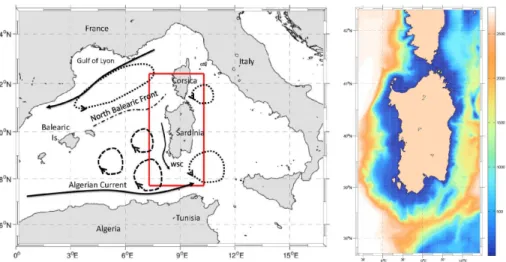
seas around Sardinia, which is a highly variable and dynamic area crossed by several

(sub-)mesoscale structures of different origin (Fuda et al., 2000; Puillat et al., 2002;

Ribotti et al., 2004; Testor et al., 2005) and also affected by strong wind events having

both high-frequency (days-weeks) and seasonal (winter) periodicity in their peaks. The Sardinian Sea, i.e. the continental shelf and offshore area west of Sardinia, 5

is part of the Algero-Provençal Basin. From the basin scale circulation perspective, the Sardinian sea is located in between the Algerian Basin at south, dominated by the inflow of Atlantic water from Gibraltar advected by the Algerian Current, and the Provençal Basin at north characterized by the path of the Northern Current (Millot et al., 1999) moving southwestward along the continental shelf and where a surface cyclonic 10

gyre drives the northern sub-basin circulation Lévy et al. (1998). The southern branch of this cyclonic gyre contributes to the formation of the North Balearic front (Fuda et al., 2000; Testor and Gascard, 2003; Olita et al., 2014) which represents the separation between the Atlantic waters reservoir of the Algerian Basin and the saltier and denser waters of the Provençal basin (e.g. Olita et al., 2014). In a recent paper (Olita et al., 15

2013) we suggested, through the analysis of the outputs of a 3-D assimilative model, that the upwelling occurring along the SW Sardinian coast was pre-conditioned by the presence of a quasi-permanent southward current (Western Sardinian Current – WSC) which origin was in part due to the approaching of anticyclonic eddies to the western Sardinia shelf. This was also supported by the findings of Pinardi et al. (2013) 20

where the same current (they called Southerly Sardinia Current – SSC) is described as permanent at low-frequency scales (decadal) bordering a northern branch of the Atlantic water flow in the Western Mediterranean. In the southern parth of the model domain, south of Sardinia, the Sardinian Channel connects Thyrrennian and Algerian sub-basins. Here the Algerian Current (e.g. Millot et al., 1999) transports Atlantic wa-25

(6)

OSD

12, 1–30, 2015

surface fluxes

A. Olita et al.

Title Page

Tables Figures

◭ ◮

Back Close

Full Screen / Esc

Discussion

P

a

per

|

Discussion

P

a

per

|

Discussion

P

a

per

|

Discussion

P

a

per

et al., 1999) in the northern Thyrrenian sea, east of Sardinia, that represents the most energetic mesoscale structure of the northern Thyrrenian sea (Iacono et al., 2013).

This area would be likely one of the most influenced by different estimations of wind

stress, considering the relevance that winds has in the local circulation.

All these characteristics make this domain a good test case to study the impact of the 5

inclusion of surface currents on the surface fluxes (with special regards to momentum) and their feedback on circulation at local scales.

The aim of the present work is to study the impact of the surface currents in the com-putation of the surface momentum and heat fluxes, through the bulk formulas (Fairall et al., 2003), in turn driving surface and sub-surface dynamics and temperature. The 10

latter can be modified both directly through changes in surface heat fluxes but also as consequences of variations in vertical motions. To evaluate such an impact, we per-formed a twin experiment with the Regional Ocean Modelling System (ROMS). ROMS was implemented in the Sardinian at 2 km of horizontal resolution and 30 s vertical lev-els. Details of the model implementation are provided in Sect. 2, together with details on 15

observational data used and analyses performed. Two experiments were conducted, both simulating the year 2012, with and without the contribution of surface currents in the computation of the momentum and heat fluxes. In Sect. 3 we validate the model

and compare the outcomes of the two setups under different points of view. Finally,

concluding remarks are drawn in Sect. 4. 20

2 Methods and data

2.1 Numerical model and experiments

The numerical model is an implementation of the Regional Ocean Modeling System (ROMS Shchepetkin and McWilliams, 2003, 2005). ROMS is a free surface,

hydro-static, primitive equation, finite di_fference model that is widely used by the scientific

25

(7)

Haid-OSD

12, 1–30, 2015

surface fluxes

A. Olita et al.

Title Page

Tables Figures

◭ ◮

Back Close

Full Screen / Esc

Discussion

P

a

per

|

Discussion

P

a

per

|

Discussion

P

a

per

|

Discussion

P

a

per

|

vogel et al., 2000), ecological modelling (Dinniman et al., 2003), coastal studies (e.g. Wilkin et al., 2005; Iermano et al., 2012), sea-ice modelling and many others. The model was implemented in the seas around Sardinia (Fig. 1) in a rectangular grid of 2 km of nominal resolution on the horizontal plane and 30 s terrain following lev-els. The equation distributing vertical levels allows a robust description of surface and 5

subsurface layers where most of the dynamical processes occur while intermediate and deep layers are discretized with larger meshes. The US Navy Digital Bathymetry Database at 1 min of resolution was interpolated on the model horizontal grid. So ob-tained bathymetry was also smoothed in order to minimize the pressure gradient force (PGF) error often caused by too steep bathymetric gradients.

10

Initial conditions as well as boundary conditions were provided by the 1/16◦ model

of the Mediterranean Sea MFS-1671 (Tonani et al., 2009) retrieved through My-Ocean (www.myocean.eu) data portal. Daily analyses 3-D fields of velocities, temperature, salinity and elevation (2-D) have been used for model nesting and initialization. At the boundary the model uses Flather conditions (Flather, 1976) for the barotropic veloc-15

ities while baroclinic velocities and 3-D tracers (T and S) are clamped to the values prescribed by the outer model. At the free surface the Chapman (Chapman, 1985) boundary condition was imposed. A third-order upstream horizontal advection of

3-D momentum (Shchepetkin and McWilliams, 1998) and the k−ǫ turbulence closure

scheme (Warner et al., 2005) were used in the present implementation. At surface, 20

which is the focus of the present work, we used the 1/8◦6 hourly ECMWF ERA-interim

analyses fields. 10 m air temperature, U and V wind momentum components, air pres-sure, solar shortwave radiation, air humidity and precipitation were used to compute freshwater, momentum and heat fluxes by using the above cited bulk formulas.

2.2 Experiments

25

Two experiments were performed: experimentBulk Fluxes(BF) did not include surface

currents (so in Eqs. 1, 2 and 3 theus term was neglected), while in Bulk Fluxes with

(8)

repro-OSD

12, 1–30, 2015

surface fluxes

A. Olita et al.

Title Page

Tables Figures

◭ ◮

Back Close

Full Screen / Esc

Discussion

P

a

per

|

Discussion

P

a

per

|

Discussion

P

a

per

|

Discussion

P

a

per

duced by the model. The simulations were integrated for 1 year, simulating the year 2012 with the model forced at boundaries and surface by the above described realistic fields. It deserves a little discussion the issue related to the data assimilation. Consid-ering that the model boundaries are provided by an assimilative model we think that for such a small domain the information contained in the boundaries would propagate 5

to the nested model without a substantial loss of information. On the contrary for larger

off-line nested domains literature (Vandenbulcke et al., 2006; Olita et al., 2012)

sug-gest that assimilation is needed to improve the simulation. Further, and maybe more important, as in the present work we are interested to observe changes generated

by different parametrizations of physical phenomena we should avoid any important

10

statistical correction of the model results as the Data Assimilation procedures do.

Fu-ture efforts will be devoted to study impacts of Data assimilation in such small coastal

domains nested to assimilative models.

2.3 Validation data and metrics

Model performances were assessed by using satellite SST fields. Satellite SST used 15

are the MyOcean sea surface temperature nominal operational product for the Mediter-ranean Sea available from http://www.myocean.eu. Product used are the daily gap-free

maps (L4) at 1/16◦ of resolution. The data are obtained from infrared measurements

collected by satellite radiometers and statistical interpolation (Optimal Interpolation). Three basic metrics, namely Bias, Root Mean Square Error (RMSE) and Anomaly 20

Correlation Coe_fficient (ACC) provide a good overview of the quality of the model in

reproducing the observed SST. While RMSE and BIAS describe the model error in reproducing observed value of the considered variable, ACC measures of the ability of the model in reproducing anomalies of the SST signature detected by the satellite, partly overlooking their absolute value. In this perspective it can be also considered an 25

(9)

OSD

12, 1–30, 2015

surface fluxes

A. Olita et al.

Title Page

Tables Figures

◭ ◮

Back Close

Full Screen / Esc

Discussion

P

a

per

|

Discussion

P

a

per

|

Discussion

P

a

per

|

Discussion

P

a

per

|

The three metrics are formulated as follows:

BIAS= 1

N

X

i=1

(obs_i−mod_i), (4)

RMSE₌

v u u

t1

N

X

i=1

(obs_i−mod_i)2_, ₍₅₎

ACC=

N

P

i=1

(mod_i−obs_i)(obs_i−obs_i)

s

N

P

i=1

(mod_i−obs_i)2PN

i=1

(obs_i−obs_i)2

, (6)

where mod and obs are respectively modeled and observed values of the variable 5

and the overbar indicates a long-term temporal average. In the present paper this long temporal average is the AVHRR monthly climatology (1982–2008). This allowed to

filter off the seasonal signal that otherwise would hide the response of this metric to

the synoptic features. ACC is an adimensional number ranging from−1 (worst) to₊1

(best). 10

2.3.1 Flow decomposition, kinetics and work

In order to investigate the impact of the different parametrizations of the surface fluxes

on the simulated dynamics, we separated the stable and the fluctuating part of the velocities as already described for example in Olita et al. (2013). The time-averaged

termu=hui+u′ represents the stable part of the flow, whileu′ is its fluctuating part.

15

The fluctuating components can be used to describe both Eddy Kinetic Energy (EKE₌

1/2(u′2+v′2)) and the Reynolds Stress covariance term (RS=u′v′) also known as

(10)

OSD

12, 1–30, 2015

surface fluxes

A. Olita et al.

Title Page

Tables Figures

◭ ◮

Back Close

Full Screen / Esc

Discussion

P

a

per

|

Discussion

P

a

per

|

Discussion

P

a

per

|

Discussion

P

a

per

the flow interacts with the mean flow, accelerating or deflecting it from its mean direction (Greatbatch et al., 2010). It is likely that changes in surface parametrization of surface

fluxes would influence both the stable and the fluctuating part of the flow, but in different

measure. This suggested us to investigate the two separately.

Wind stress workP, which is defined as the product of wind stressτ by the surface

5

ocean currents u_s was computed in order to assess the differences in terms of wind

power input to the ocean between the two model experiments. At oceanic scales, it was estimated a reduction of about 20–30 % when accounting for surface currents contribution in wind stress computation (Duhaut and Straub, 2006; Hughes and Wilson, 2008).

10

3 Results and discussion

3.1 SST validation and intercomparison

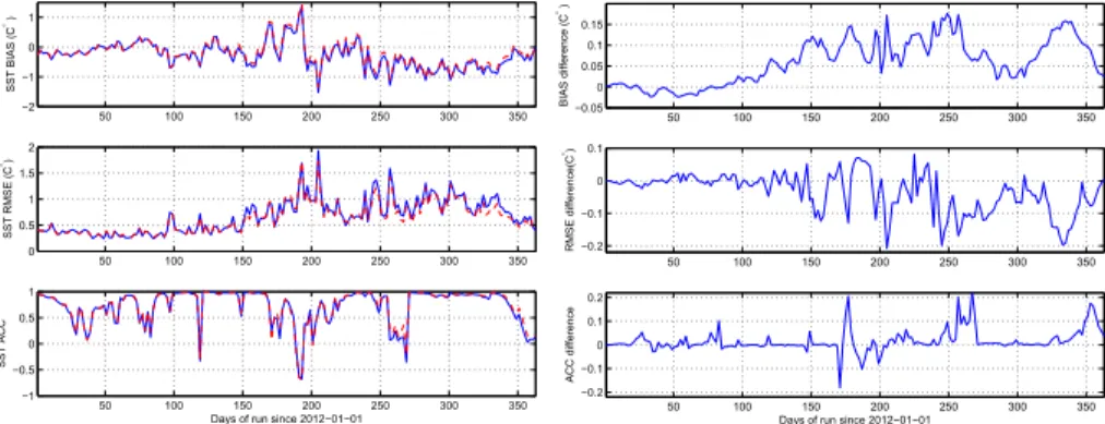
Figure 2 shows the three time series for SST RMSE, BIAS and ACC metrics computed vs the SST data as described in methods section.

Such spatially averaged metrics do not show dramatic differences between the two

15

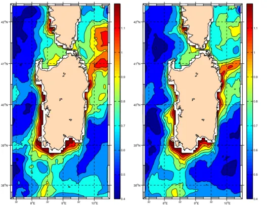
setups. However, BFC (i.e. with currents) setup shows slightly better performances than BF for all the three metrics (see right panel of Fig. 2). Of course, considering the complexity of topography, bathymetry and dynamics of the study area, a strong spatial variability of RMSE’s values would be expected. Actually RMSE maps (Fig. 3) for BF and BFC experiments show a quite large variability of the RMSE over space. Major 20

improvements for BFC setup are located in the area of cyclonic circulation just east the Bonifacio strait. Other small but significant (because probably connected to important surface features as the Western Sardinia Current) improvements are shown close to the western coast, where a narrow coastal band with large RMSE is quite reduced both in width and magnitude in the BFC experiment.

(11)

OSD

12, 1–30, 2015

surface fluxes

A. Olita et al.

Title Page

Tables Figures

◭ ◮

Back Close

Full Screen / Esc

Discussion

P

a

per

|

Discussion

P

a

per

|

Discussion

P

a

per

|

Discussion

P

a

per

|

3.2 Impact on surface fluxes

Accordingly to the bulk formulas of Eq. (1), the largest direct impact should be observed for the momentum flux as the relative wind has a quadratic relation with wind stress. A lower impact is supposed to be observed for sensible and latent fluxes, where the relative wind velocity account for a linear relation with fluxes. All the three fluxes (see 5

Fig. 4) show an impact that in percentage terms is of the order of few percentage points

(∼ −2 %) by averaging time series values, but with a distinct high frequency behaviour

showing a large temporal and also suggesting a large spatial variability.

The small differences in terms of time series underneath quite large differences in

space because of the very nature of the fluxes and the way they are computed (i.e. 10

interactively during the model integration and with a feedback to ocean currents for BFC experiment). In this regard a significant information is provided by the time-averaged

difference map between BFC and BF wind stress fluxes represented in Fig. 5.

Such spatial differences peak−7×10−3N m−2in the proximity of the southern

bound-ary of the domain where the highly unstable Algerian Current flows and also in the turn-15

ing point of the Western Sardinia Current in the SW corner of Sardinia. Positive patches

are less present, reaching a maximum of∼ 2×10−3N m−2. In percentage terms these

spatial differences range between −15 % and +20 % on the annual basis, while are

obsiously larger considering the daily basis. The values of heat fluxes difference (right

panel of Fig. 5) seem to be directly related to the improved model performances (as 20

shown in Fig. 3) east of the Bonifacio strait. In correspondence of the cyclonic gyre east of Bonifacio the map shows the largest correction in terms of heat fluxes, with a relatively “large” reduction of such a flux. Another one is the large cyclonic circulation area located in the SE margin of the domain (named South Eastern Sardinian Gyre by Sorgente et al., 2011).

(12)

OSD

12, 1–30, 2015

surface fluxes

A. Olita et al.

Title Page

Tables Figures

◭ ◮

Back Close

Full Screen / Esc

Discussion

P

a

per

|

Discussion

P

a

per

|

Discussion

P

a

per

|

Discussion

P

a

per

3.3 Impact on the mean and turbulent surface circulation

The above seen changes in wind stress would likely generate significant changes in surface kinetics and/or circulation. Figure 6 shows time series of total kinetic and eddy kinetic energy for the two experiments. Comparing the time series is evident that the introduction of the currents on stress computation (BFC) led to a spatially-averaged 5

reduction of the kinetic energies at surface. Such a reduction, which accounts for about

−17 %, shows a long period maximum between days 60 and 120, i.e. during March

and April, when BF surface kinetics almost double BFC ones. The largest part of such

difference between total kinetic energies at surface (about 65 %) is actually due to the

turbulent part of the flow. Eddy kinetic energy shows the same behaviour as the total 10

one, with maximum difference between the two experiments also during spring.

Time-averaged maps of the above quantities provide an insight of the distribution of

such differences.

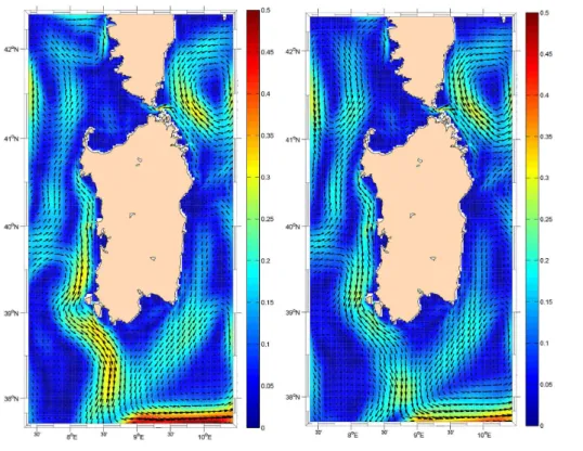
Although the mean flow (Fig. 7) does not show appreciable differences in terms of

path, it reveals an important reduction (about 15 %) in the averaged velocity module 15

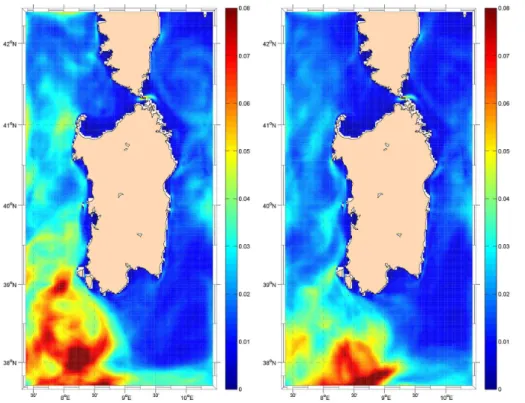
for BFC experiment. On the other side, EKE maps (Fig. 8) reveal that a large part of

such differences can be ascribed to the fluctuating part of the circulation as already

argued by observing the time series. The south-western area shows the largest diff

er-ences between the two EKE estimates. Useful information is provided by comparing Reynolds stress covariance maps (Fig. 9): the map for BF experiments shows a neat 20

circular area in the SW corner of the domain with alternating negative and positive values, which is a typical eddy footprint. This signature partially disappears in BFC: the alternance of such negative and positive patches appears only close to the coast, likely to be due to the previously mentioned WSC that here strongly interacts with to-pography and deviates its southward path towards east. Such a south-western area is 25

(13)

OSD

12, 1–30, 2015

surface fluxes

A. Olita et al.

Title Page

Tables Figures

◭ ◮

Back Close

Full Screen / Esc

Discussion

P

a

per

|

Discussion

P

a

per

|

Discussion

P

a

per

|

Discussion

P

a

per

|

a consequent change in the transfer of energy from the eddy to the mean flow. Lower turbulent energy, that can be clearly desumed by comparing the two maps of eddy ki-netic energy, could influence vertical dynamics in the SW area where the local coastal upwelling was previously (Olita et al., 2013) found to be preconditioned by the WSC intensity and by eddies interacting with the continental slope.

5

3.4 Vertical dynamics

Comparison of the maps of Fig. 10 emphasizes the differences in vertical velocitiesw

between the two setups. In those mapsw velocities are interpolated at−50 m of depth

and averaged over the whole period. We get vertical velocities for such a depth in order

to avoid the noisyw signal characterizing the (turbulent) mixed layer in agreement to

10

what was done by Jacox et al. (2014) to describe the California Current upwelling.

Comparing BF with BFC setup, the upwelling area slightly differ being a little large for

BF (warm color in the map). However, the largest difference between the two simulation

is in terms of intensity of the upwelling. In BF experiments many upwelling patches

easily overpass 5 m day−1reaching up to 10 m day−1, while in BFC the values are quite

15

lower, reaching at most 6–7 m day−1with larger areas recording values of 2–4 m day−1.

It is hard to evaluate who is more realistic, but we are confident that the lower estimate (BFC) is the best one in the light of the better performances in terms of SST RMSE and

also considering that 10 m day−1is quite a large estimate if compared with bibliography

that records such values (or even lower) for synoptic scales (e.g. Tintoré et al., 1991). 20

4 Conclusions

(14)

OSD

12, 1–30, 2015

surface fluxes

A. Olita et al.

Title Page

Tables Figures

◭ ◮

Back Close

Full Screen / Esc

Discussion

P

a

per

|

Discussion

P

a

per

|

Discussion

P

a

per

|

Discussion

P

a

per

Mediterranean Sea) by using two different setups, with and without the contribute of

currents in the computation of surface fluxes through bulk formulas.

Accordingly to bibliography (which was mainly related to oceanic and basin scales) we found a changes in momentum and net heat fluxes of some percentage points

while more consistent differences are found for surface kinetic energies (BFC records

5

a 10 % reduction on total surface kinetic enrgy in respect to BF). Differences can be

observed both in the mean as well in the fluctuating part of the flow. In particular the dynamical field changed in its fluctuating part in the SW corner of the domain, in the area of interaction between anticyclonic eddies formed along the Algerian Current and the continental shelf.

10

Inclusion of surface currents determined relevant changes not only in dynamics but also in the prognosed surface temperature by means of the surface heat fluxes. Valida-tion with satellite SST revealed that the simulaValida-tion in areas characterized by cyclonic structures benefits by such a modification in heat fluxes, largely reducing the error (RMSE) in respect to observations.

15

While quantitative metrics for SST reveal that net heat fluxes and resulting SST are improved, it is unclear (i.e. not quantitatively validated) if, at these scales, the use of relative winds brings quality to the simulated dynamics or not. Comparison of synoptic satellite infrared and optic observations with modeled results did not solve the issue: this is probably due to dynamical changes that are higher in magnitude than in spatial 20

distribution and then hardly detectable from signatures in surface optic/infrared obser-vations (not shown). However, the comparison of vertical dynamics suggest that more realistic values are provided when the model takes into account surface currents com-ponent in stress formulation.

From a process oriented perspective, observed reduction of coastal upwelling in the 25

(15)

OSD

12, 1–30, 2015

surface fluxes

A. Olita et al.

Title Page

Tables Figures

◭ ◮

Back Close

Full Screen / Esc

Discussion

P

a

per

|

Discussion

P

a

per

|

Discussion

P

a

per

|

Discussion

P

a

per

|

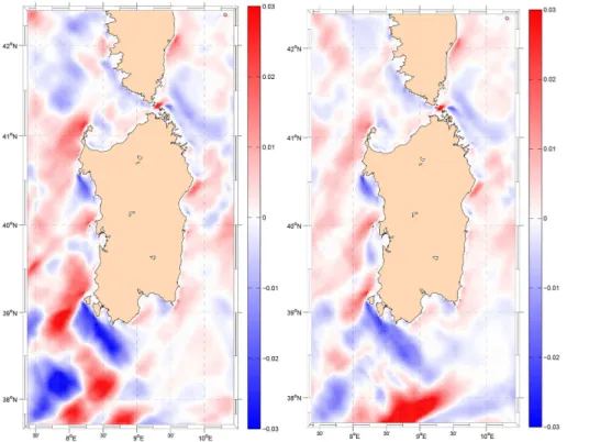
Wind stress work, the product of wind stress and ocean surface currents, provides an insight of the wind power input to the ocean. Such an input is reduced for about 15 % as

basin averages, with absolute spatial differences between the two estimates are shown

in Fig. 11. It is quite evident that power input to sea surface is noticeably reduced in the area of the Western Sardinian Current. So it is probable that such current would 5

be overestimated when not accounting for the feeback of the current itself on surface momentum flux.

More in general the study suggests that, also at regional and coastal scales, the contribution of surface currents should not be neglected in the computation of both heat and momentum fluxes at air/sea interface in ocean models, also considering 10

the negligible computational cost. This is especially true for areas highly populated by (sub-)mesoscale and other coastal processes (as the upwelling for example) that in-crease the variability of both currents and tracer fields, then requiring a higher accuracy in resolving underlying physical processes.

Acknowledgements. This work has been funded by the Italian Flagship Project RITMARE and

15

by the Italian Project PON-TESSA (C. U. PON01-02823), both funded by the Italian Ministry for Research – MIUR. Initial and boundary conditions as well as data for validation have been provided by the MyOcean data portal (http://www.myocean.eu) realized through EU projects MyOcean and MyOcean2 funded by VII FP SPACE (contracts 218812 and 283367).

References

20

Chapman, D. C.: Numerical treatment of cross-shelf open boundaries in a Barotropic Coastal Ocean Model, J. Phys. Oceanogr., 15, 1060–1075, doi:10.1175/1520-0485(1985)015<1060:NTOCSO>2.0.CO;2, 1985. 7

Dawe, J. T. and Thompson, L.: Effect of ocean surface currents on wind stress, heat flux, and wind power input to the ocean, Geophys. Res. Lett., 33, L09604,

25

(16)

OSD

12, 1–30, 2015

surface fluxes

A. Olita et al.

Title Page

Tables Figures

◭ ◮

Back Close

Full Screen / Esc

Discussion

P

a

per

|

Discussion

P

a

per

|

Discussion

P

a

per

|

Discussion

P

a

per

Deng, Z., Xie, L., Liu, B., Wu, K., Zhao, D., and Yu, T.: Coupling winds to ocean surface currents over the global ocean, Ocean Model., 29, 261–268, doi:10.1016/j.ocemod.2009.05.003, 2009. 4

Dinniman, M. S., Klinck, J. M., and Smith, W. O.: Cross-shelf exchange in a model of the Ross Sea circulation and biogeochemistry, Deep-Sea Res. Pt. II, 50, 3103–3120,

5

doi:10.1016/j.dsr2.2003.07.011, 2003. 7

Duhaut, T. H. A. and Straub, D. N.: Wind stress dependence on ocean surface velocity: im-plications for mechanical energy input to ocean circulation, J. Phys. Oceanogr., 36, 202, doi:10.1175/JPO2842.1, 2006. 4, 10

Fairall, C. W., Bradley, E. F., Rogers, D. P., Edson, J. B., and Young, G. S.: Bulk

parameteri-10

zation of air-sea fluxes for Tropical Ocean-Global Atmosphere Coupled-Ocean Atmosphere Response Experiment, J. Geophys. Res., 101, 3747–3764, doi:10.1029/95JC03205, 1996. 3

Fairall, C. W., Bradley, E. F., Hare, J. E., Grachev, A. A., and Edson, J. B.: Bulk parameterization of air sea fluxes: updates and verification for the COARE algorithm, J. Climate, 16, 571–591,

15

doi:10.1175/1520-0442(2003)016<0571:BPOASF>2.0.CO;2, 2003. 3, 6

Flather, R. A.: A tidal model of the northwest European continental shelf, Mem. Soc. R. Sci. Liege, 6, 141–164, 1976. 7

Fuda, J., Millot, C., Taupier-Letage, I., Send, U., and Bocognano, J.: XBT monitoring of a merid-ian section across the western Mediterranean Sea, Deep-Sea Res. Pt. I, 47, 2191–2218,

20

2000. 5

Greatbatch, R. J., Zhai, X., Kohlmann, J.-D., and Czeschel, L.: Ocean eddy momentum fluxes at the latitudes of the Gulf Stream and the Kuroshio extensions as revealed by satellite data, Ocean Dynam., 60, 617–628, doi:10.1007/s10236-010-0282-6, 2010. 10

Haidvogel, D. B., Arango, H. G., Hedstrom, K., Beckmann, A., Malanotte-Rizzoli, P., and

25

Shchepetkin, A. F.: Model evaluation experiments in the North Atlantic Basin: simula-tions in nonlinear terrain-following coordinates, Dynam. Atmos. Oceans, 32, 239–281, doi:10.1016/S0377-0265(00)00049-X, 2000. 6

Hughes, C. W. and Wilson, C.: Wind work on the geostrophic ocean circulation: an observa-tional study of the effect of small scales in the wind stress, J. Geophys. Res.-Oceans, 113,

30

(17)

OSD

12, 1–30, 2015

surface fluxes

A. Olita et al.

Title Page

Tables Figures

◭ ◮

Back Close

Full Screen / Esc

Discussion

P

a

per

|

Discussion

P

a

per

|

Discussion

P

a

per

|

Discussion

P

a

per

|

Iacono, R., Napolitano, E., Marullo, S., Artale, V., and Vetrano, A.: Seasonal variability of the tyrrhenian sea surface geostrophic circulation as assessed by altimeter data, J. Phys. Oceanogr., 43, 1710–1732, 2013. 6

Iermano, I., Liguori, G., Iudicone, D., Buongiorno Nardelli, B., Colella, S., Zingone, A., Saggiomo, V., and Ribera d’Alcalà, M.: Filament formation and evolution in

buoy-5

ant coastal waters: Observation and modelling, Prog. Oceanogr., 106, 118–137, doi:10.1016/j.pocean.2012.08.003, 2012. 7

Jacox, M. G., Moore, A. M., Edwards, C. A., and Fiechter, J.: Spatially resolved upwelling in the California Current System and its connections to climate variability, Geophys. Res. Lett., 41, 3189–3196, doi:10.1002/2014GL059589, 2014. 13

10

Kara, A. B., Metzger, E. J., and Bourassa, M. A.: Ocean current and wave effects on wind stress drag coefficient over the global ocean, Geophys. Res. Lett., 34, L01604, doi:10.1029/2006GL027849, 2007. 4

Lévy, M., Memery, L., and Madec, G.: The onset of a bloom after deep winter convection in the northwestern Mediterranean sea: mesoscale process study with a primitive equation model,

15

J. Marine Syst., 16, 7–21, 1998. 5

Millot, C., Gacic, M., Astraldi, M., and La Violette, P. E.: Circulation in the Western Mediter-ranean Sea, J. Marine Syst., 20, 423–442, 1999. 5

Olita, A., Dobricic, S., Ribotti, A., Fazioli, L., Cucco, A., Dufau, C., and Sorgente, R.: Impact of SLA assimilation in the Sicily Channel Regional Model: model skills and mesoscale features,

20

Ocean Sci., 8, 485–496, doi:10.5194/os-8-485-2012, 2012. 8

Olita, A., Ribotti, A., Fazioli, L., Perilli, A., and Sorgente, R.: Surface circulation and upwelling in the Sardinia Sea: A numerical study, Cont. Shelf. Res., 71, 95–108, doi:10.1016/j.csr.2013.10.011, 2013. 5, 9, 13

Olita, A., Sparnocchia, S., Cusí, S., Fazioli, L., Sorgente, R., Tintoré, J., and Ribotti, A.:

Obser-25

vations of a phytoplankton spring bloom onset triggered by a density front in NW Mediter-ranean, Ocean Sci., 10, 657–666, doi:10.5194/os-10-657-2014, 2014. 5

Perilli, A., Rupolo, V., and Salusti, E.: Satellite investigations of a cyclonic gyre in the cen-tral Tyrrhenian Sea (western Mediterranean Sea), J. Geophys. Res., 100, 2487–2499, doi:10.1029/94JC01315, 1995. 5

30

(18)

ret-OSD

12, 1–30, 2015

surface fluxes

A. Olita et al.

Title Page

Tables Figures

◭ ◮

Back Close

Full Screen / Esc

Discussion

P

a

per

|

Discussion

P

a

per

|

Discussion

P

a

per

|

Discussion

P

a

per

rospective analysis, Prog. Oceanogr., online first, doi:10.1016/j.pocean.2013.11.003, 2013. 5

Puillat, I., Taupier-Letage, I., and Millot, C.: Algerian eddies lifetime can near 3 years, J. of Marine Systems, 31, 245–259, 2002. 5

Ribotti, A., Puillat, I., Sorgente, R., and Natale, S.: Mesoscale circulation in the surface layer off

5

the southern and western Sardinia Island in 2000–2002, Chem. Ecol., 20, 345–363, 2004. 5 Shchepetkin, A. F. and McWilliams, J. C.: Quasi-monotone advection schemes based on explicit locally adaptive dissipation, Mon. Weather Rev., 126, 1541, doi:10.1175/1520-0493(1998)126<1541:QMASBO>2.0.CO;2, 1998. 7

Shchepetkin, A. F. and McWilliams, J. C.: A method for computing horizontal pressure-gradient

10

force in an oceanic model with a nonaligned vertical coordinate, J. Geophys. Res.-Oceans, 108, 3090, doi:10.1029/2001JC001047, 2003. 6

Shchepetkin, A. F. and McWilliams, J. C.: The regional oceanic modeling system (ROMS): a split-explicit, free-surface, topography-following-coordinate oceanic model, Ocean Model., 9, 347–404, doi:10.1016/j.ocemod.2004.08.002, 2005. 6

15

Sorgente, R., Olita, A., Oddo, P., Fazioli, L., and Ribotti, A.: Numerical simulation and decom-position of kinetic energy in the Central Mediterranean: insight on mesoscale circulation and energy conversion, Ocean Sci., 7, 503–519, doi:10.5194/os-7-503-2011, 2011. 11

Testor, P. and Gascard, J.-C.: Large-scale spreading of deep waters in the Western Mediterranean Sea by submesoscale coherent eddies, J. Phys. Oceanogr., 33, 75–87,

20

doi:10.1175/1520-0485(2003)033<0075:LSSODW>2.0.CO;2, 2003. 5

Testor, P., Béranger, K., and Mortier, L.: Modeling the deep eddy field in the southwest-ern Mediterranean: the life cycle of Sardinian eddies, Gephys. Res. Lett., 32, L13602, doi:10.1029/2004GL022283, 2005. 5

Tintoré, J., Gomis, D., Alonso, S., and Parrilla, G.: Mesoscale dynamics and vertical motion in

25

the Alborán Sea, J. Phys. Oceanogr., 21, 811–823, 1991. 13

Tonani, M., Pinardi, N., Fratianni, C., Pistoia, J., Dobricic, S., Pensieri, S., de Alfonso, M., and Nittis, K.: Mediterranean Forecasting System: forecast and analysis assessment through skill scores, Ocean Sci., 5, 649–660, doi:10.5194/os-5-649-2009, 2009. 7

Vandenbulcke, L., Barth, A., Rixen, M., Alvera-Azcarate, A., Ben Bouallegue, Z., and

Beck-30

(19)

OSD

12, 1–30, 2015

surface fluxes

A. Olita et al.

Title Page

Tables Figures

◭ ◮

Back Close

Full Screen / Esc

Discussion

P

a

per

|

Discussion

P

a

per

|

Discussion

P

a

per

|

Discussion

P

a

per

|

Warner, J. C., Sherwood, C. R., Arango, H. G., and Signell, R. P.: Performance of four turbulence closure models implemented using a generic length scale method, Ocean Model., 8, 81–113, doi:10.1016/j.ocemod.2003.12.003, 2005. 7

Wilkin, J. L., Arango, H. G., Haidvogel, D. B., Lichtenwalner, C. S., Glenn, S. M., and Hed-ströM, K. S.: A regional ocean modeling system for the long-term ecosystem observatory, J.

5

Geophys. Res.-Oceans, 110, C06S91, doi:10.1029/2003JC002218, 2005. 7

(20)

OSD

12, 1–30, 2015

surface fluxes

A. Olita et al.

Title Page

Tables Figures

◭ ◮

Back Close

Full Screen / Esc

Discussion

P

a

per

|

Discussion

P

a

per

|

Discussion

P

a

per

|

Discussion

P

a

per

Figure 1.Left: Study area with toponyms and main circulation features as known from literature.

(21)

OSD

12, 1–30, 2015

surface fluxes

A. Olita et al.

Title Page

Tables Figures

◭ ◮

Back Close

Full Screen / Esc

Discussion

P

a

per

|

Discussion

P

a

per

|

Discussion

P

a

per

|

Discussion

P

a

per

|

50 100 150 200 250 300 350

0 0.5 1 1.5 2

SST RMSE (C

°)

50 100 150 200 250 300 350

−1 −0.5 0 0.5 1

SST ACC

Days of run since 2012−01−01

50 100 150 200 250 300 350

−2 −1 0 1

SST BIAS (C

° )

50 100 150 200 250 300 350

−0.2 −0.1 0 0.1

RMSE difference(C

°)

50 100 150 200 250 300 350

−0.2 −0.1 0 0.1 0.2

ACC difference

Days of run since 2012−01−01

50 100 150 200 250 300 350

−0.05 0 0.05 0.1 0.15

BIAS difference (C

°)

Figure 2.Left: BIAS, RMSE and ACC for BF (blue) and BFC (red dashed) experiments. Right:

(22)

OSD

12, 1–30, 2015

surface fluxes

A. Olita et al.

Title Page

Tables Figures

◭ ◮

Back Close

Full Screen / Esc

Discussion

P

a

per

|

Discussion

P

a

per

|

Discussion

P

a

per

|

Discussion

P

a

per

30’

8o

E 30’

9o

E 30’

10o

E 38o

N 39o

N 40o

N 41o

N 42oN

0.4 0.5 0.6 0.7 0.8 0.9 1 1.1

30’

8o

E 30’

9o

E 30’

10o

E 38o

N 39o

N 40o

N 41o

N 42oN

0.4 0.5 0.6 0.7 0.8 0.9 1 1.1

(23)

OSD

12, 1–30, 2015

surface fluxes

A. Olita et al.

Title Page

Tables Figures

◭ ◮

Back Close

Full Screen / Esc

Discussion

P

a

per

|

Discussion

P

a

per

|

Discussion

P

a

per

|

Discussion

P

a

per

|

50 100 150 200 250 300 350

−15 −10 −5

0x 10 −3

WS (N/m

2)

50 100 150 200 250 300 350

−3 −2 −1 0 1

SHF (W/m

2)

50 100 150 200 250 300 350

−4 −2 0 2

LHF (W/m

2)

50 100 150 200 250 300 350

−8 −6 −4 −2 0 2 4

NHF (W/m

2)

Days since 2012−01−01

Figure 4.Top to bottom: wind stress, sensible, latent and net heat fluxes differences between

(24)

OSD

12, 1–30, 2015

surface fluxes

A. Olita et al.

Title Page

Tables Figures

◭ ◮

Back Close

Full Screen / Esc

Discussion

P

a

per

|

Discussion

P

a

per

|

Discussion

P

a

per

|

Discussion

P

a

per

Figure 5.Difference map (BFC – BF) of the time-averaged wind stress (left) and net heat

(25)

OSD

12, 1–30, 2015

surface fluxes

A. Olita et al.

Title Page

Tables Figures

◭ ◮

Back Close

Full Screen / Esc

Discussion

P

a

per

|

Discussion

P

a

per

|

Discussion

P

a

per

|

Discussion

P

a

per

|

0 50 100 150 200 250 300 350 400 0.015

0.02 0.025 0.03 0.035 0.04 0.045 0.05 0.055 0.06 0.065

Surface KE (m

2/s 2)

surface kinetic energy

BF BFC

0 50 100 150 200 250 300 350 400 0.01

0.015 0.02 0.025 0.03 0.035 0.04 0.045 0.05 0.055

Surface EKE (m

2/s 2)

surface eddy kinetic energy

BF BFC

Figure 6.Total (left) and Turbulent Kinetic Energy at surface. Red curve is for BF and green for

(26)

OSD

12, 1–30, 2015

surface fluxes

A. Olita et al.

Title Page

Tables Figures

◭ ◮

Back Close

Full Screen / Esc

Discussion

P

a

per

|

Discussion

P

a

per

|

Discussion

P

a

per

|

Discussion

P

a

per

(27)

OSD

12, 1–30, 2015

surface fluxes

A. Olita et al.

Title Page

Tables Figures

◭ ◮

Back Close

Full Screen / Esc

Discussion

P

a

per

|

Discussion

P

a

per

|

Discussion

P

a

per

|

Discussion

P

a

per

|

(28)

OSD

12, 1–30, 2015

surface fluxes

A. Olita et al.

Title Page

Tables Figures

◭ ◮

Back Close

Full Screen / Esc

Discussion

P

a

per

|

Discussion

P

a

per

|

Discussion

P

a

per

|

Discussion

P

a

per

(29)

OSD

12, 1–30, 2015

surface fluxes

A. Olita et al.

Title Page Abstract Introduction Conclusions References Tables Figures ◭ ◮ ◭ ◮ Back Close

Full Screen / Esc

Printer-friendly Version Interactive Discussion Discussion P a per | Discussion P a per | Discussion P a per | Discussion P a per | 40’ 8o

E 20’ 40’

9o E 40’ 39o N 20’ 40’ 40o N 40’ 8o

E 20’ 40’

9o E 40’ 39o N 20’ 40’ 40o N −10 −8 −6 −4 −2 0 2 4 6 8 10 40’ 8o

E 20’ 40’

9o E 40’ 39o N 20’ 40’ 40o N 40’ 8o

E 20’ 40’

9o E 40’ 39o N 20’ 40’ 40o N −10 −8 −6 −4 −2 0 2 4 6 8 10

Figure 10.Vertical velocities at−50 m depth averaged over the whole period for BF (left) and

(30)

OSD

12, 1–30, 2015

surface fluxes

A. Olita et al.

Title Page

Tables Figures

◭ ◮

Back Close

Full Screen / Esc

Discussion

P

a

per

|

Discussion

P

a

per

|

Discussion

P

a

per

|

Discussion

P

a

per

Figure 11. Wind stress work difference (BFC-BF). Units are W m−2. Blue negative patches