TOWARDS AUTOMATIC PROCESSING OF VIRTUAL CITY MODELS FOR
SIMULATIONS
R. Piepereita,∗, A. Schillingc, N. Alamb, M. Wewetzera, M. Priesa, V. Coorsb a
Beuth Hochschule f¨ur Technik Berlin University of Applied Sciences, Department II, Luxemburger Straße 10, 13353 Berlin, Germany -(rpiepereit, mwewetzer, pries)@beuth-hochschule.de
b
HFT Stuttgart University of Applied Sciences, Faculty C, Schellingstraße 24, 70174 Stuttgart, Germany -(nazmul.alam, volker.coors)@hft-stuttgart.de
cvirtualcitySYSTEMS GmbH, Tauentzienstraße 7b/c, 10789 Berlin, Germany [email protected]
KEY WORDS:3D City models processing, CityGML, STEP, B-splines, Coons, Quality
ABSTRACT:
Especially in the field of numerical simulations, such as flow and acoustic simulations, the interest in using virtual 3D models to optimize urban systems is increasing. The few instances in which simulations were already carried out in practice have been associated with an extremely high manual and therefore uneconomical effort for the processing of models. Using different ways of capturing models in Geographic Information System (GIS) and Computer Aided Engineering (CAE), increases the already very high complexity of the processing. To obtain virtual 3D models suitable for simulation, we developed a tool for automatic processing with the goal to establish ties between the world of GIS and CAE. In this paper we introduce a way to use Coons surfaces for the automatic processing of building models in LoD2, and investigate ways to simplify LoD3 models in order to reduce unnecessary information for a numerical simulation.
1. INTRODUCTION
Virtual 3D city and landscape models are mainly used for visu-alization and planning purposes nowadays. The technology for streaming and displaying huge virtual models is readily available and can be used for embedding spatial 3D assets in web pages. Many city municipalities and regional administrations are in the process of including 3D city models in their geospatial data in-frastructure. In this context, the OGC CityGML standard (Open Geospatial Consortium, 2012) has been adopted by many author-ities for storing and managing their 3D geo data sets (Kolbe, 2009). Geographic Information System (GIS) and Spatial Data Infrastructures (SDI) are well suited for documentation, distri-bution, and spatial analysis of geo data, but not for engineer-ing tasks, as for example numerical simulation. There is still a technological gap between GIS and Computed Aided Engineer-ing (CAE), which is partly due to different data capturEngineer-ing prac-tices and methods (Schilling, 2014). While engineers are mostly dealing with digital prototypes used for production, GIS data sets are created using surveying techniques such as aerial or terrestrial laser scanning. CAE tasks, such as numerical simulation, require a high degree of geometric, topologic, and semantic consistency, which detailed 3D building models as used for GIS can barely meet. Therefore, making 3D city models available to CAE in-volves not only a format conversion from 3D GIS formats such as CityGML to a CAD / CAE readable format, but also the geometry healing, preparing and optimization processes for eliminating in-consistencies in the 3D model. In many cases, a generalization is necessary because urban simulation use cases usually operate on large scale models comprising several hundreds of building ob-jects. Details such overhanging roofs, windows, doors, chimneys and other elements present in CityGML LoD3 and LoD4 models must be removed. Otherwise, the capabilities of current enter-prise workstations will not suffice for coping with the excessive number of Finite Elements involved in the physical model defini-tion.
∗Corresponding author
The aim of the research work described in this paper is to close the gap between GIS and CAE by processing virtual city mod-els with a high degree of automation in order to reduce manual effort. The implemented healing operations are applied on the CAD representation level.
For the automated processing, it has to be ensured, that the result will not falsify the outcome of a numerical simulation. Some ge-ometry features are approximated by a plurality of thin polygons, of which meshing tools of common simulation software use the edges for orientation. Thin mesh elements within these polygons can lead to numerical instability in the simulation. To avoid this instability, we used Coons surfaces for the automatic processing of building models in LoD2, as they replace a great number of thin polygons with one analytical surface.
Furthermore, we investigated ways to simplify LoD3 models, in order to reduce unnecessary information for a numerical simula-tion, without changing the simulation’s result.
The paper is organized as follows: Section 2 describes unneces-sary details of 3D building models for simulation and lists typical problems found in CityGML. A short insight into the mathemati-cal basics of B-spline surfaces and Coons surfaces is presented in section 4. In section 5, we explain in more detail the procedure for replacing polygons of LoD2 buildings with Coons surfaces. In section 3, we describe the steps for a simplification of LoD3 buildings and the occurring challenges.
2. ENABLING 3D BUILDING MODELS FOR SIMULATION
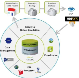
3D graphics and GIS formats. A visual inspection of the database content is enabled by an online 3D map portal, which is based on the open source Cesium.js virtual globe. Support for simulation scenarios has been added to this SDI only recently. In contrast to GIS and graphics applications, numerical simulations require different optimization methodologies, which have not been em-bedded in SDI so far. Since the involved processes cannot be supported by ETL or by OGC services, an additional branch of SDI components must be developed. Figure 1 shows how gen-eralization, geometry healing and the generation of freeform sur-faces can be attached to an already existing 3D SDI. The benefit of having a bridge between a 3D SDI and simulation frameworks is that
1. up-to-date information on the building structures is readily available for engineers working on CAE workstations,
2. time consuming manual corrections of subsets of a 3D city model becomes obsolete if all automatic geometry process-ing operations can be performed successfully,
3. scenarios and subsets can be defined by non-experts, e.g. decision-makers using an online 3D map.
Figure 1. Conceptual integration of simulation related components into a 3D SDI
When preparing CAD construction models for CAE software, a so-called de-featuring is often performed in order to reduce the model complexity and running time of the simulation. This typi-cally involves removing small drill holes, ridges, engravings, etc., which have no influence on the final simulation results. In the case of 3D building models, details such as window ledges, dec-orative elements, eaves, installations, ceilings, and so forth can often be omitted, depending on the simulation scenario. Wind simulations of entire districts, for example, work well on simpli-fied LoD2 models (according to the CityGML LoD definitions). CityGML LoD2 specifies that buildings must be represented as closed outer shells without any interiors and openings. Further-more, there must be no facade details and overhanging roofs. LoD3 models must be simplified in order to be used in numerical simulations, partly because of the model complexity, partly be-cause the separation into thematic surfaces often be-causes topolog-ical inconsistencies. Because 3D city models can be quite large
and the number of objects used for urban simulation scenarios can easily exceed one thousand, it is mandatory to fully automate the conversion and healing process, so that it can be embedded in a data preparation workflow. This workflow can then be part of a SDI with a geo database holding the entire 3D city model, so that subsets used for a simulation can be extracted on demand.
Typical geometrical / topological problems that have been found in CityGML datasets include:
• Gaps
• Holes
• Non-planar faces
• Self-intersections
• Non-manifold geometries
• Interior surfaces
• T-nodes
Figure 2 compares versions of building models without geome-try healing (left) and with geomegeome-try healing enabled (right). In contrast to approaches working directly on CityGML representa-tions and specializing in building models, as described in (Zhao et al., 2013) and (Alam et al., 2013), the healing operations imple-mented for this workflow are applied on the CAD representation level and are quite generic. Each operation, for instance fixing T-nodes, modifies only the local vicinity by deleting elements or introducing new elements and establishing new topological con-nections.
Figure 2. Geometry optimization operations on typical LoD2 building models. Top: removing interior faces. Bottom:
resolving self-intersections
3. SIMPLIFICATION OF LOD3 BUILDINGS
3.1 Simplification Process
• Investigation of surfaces which represent doors and win-dows. Identification of the surrounding wall or roof surface for projection, in which the corresponding door or window element is located.
• Determining the projection area and the corresponding poly-gons.This involves identifying the polygons in a wall or roof surface with the largest outer rings, and which contain an opening. Then calculate the surface normal of the identified projection polygons.
• Projecting the polygons of the window / door geometry on the projection surface.
• Merging of the intersected polygons type panel with the wall and merging of the type opening with the window or door opening.
• Deleting unwanted polygons (degenerated polygons, double polygons, etc.).
One of the LoD3 models used and successfully tested with the simplifications as described above is shown in Figure 3. The figure shows the original model on the right and the simplified model on the left.
Figure 3. Model simplifications of a LoD3 model
3.2 Simplification Challanges
The following section deals with some of the simplification chal-langes:
(1)
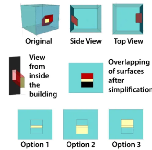
The core element of the algorithm for model simplification is the identification of the polygon within the boundary surface element on which all other polygons are to be projected. Four possible results of a simplification process in which the projection polygon is not clearly defined, are depicted in Figure 4. The options 1 to 4 show the projection on different polygons. In most cases seeking out polygons with the longest side and the largest area, and defining these as the projection polygons, will lead to a good result. Another option would be putting a bounding box around each polygon and selecting the polygon with the largest bounding box.
(2)
Figure 5 shows an example of two buildings with a loggia. The only geometrical difference is the length of the loggia. If the poly-gon is modeled around the door opening in a separate boundary surface bs2 then the loggia remains the same after the model sim-plification (option 1). In option 2 the wall surface bs1 is used as the projection surface and the door along with the loggia are projected onto the wall surface. For a very long loggia a single boundary surface might cause loss of information as is shown in building 1. On the other hand, a projection on the wall surface
Figure 4. Options for choosing the right projection surface
Figure 5. Impact of mapping the polygons to the BoundarySurfaces on the model simplification
would make more sense for a short loggia like building 2 (option 2). Ultimately, the result depends on the initial model.
(3)
When a window is positioned with an angle instead of vertically, generalization procedures could be challanging, and projecting arises redundant polygons (see Figure 6). Following are some ways to simplify: 1) The window is projected horizontally on the wall surface and the resulting redundant wall surfaces are merged and overlapping windows and surfaces will be deleted. In this case, the window remains as it is visible from the outside. 2) The window is projected horizontally on the wall and the overlapping wall surface is deleted. In this case, the window area remains the same. 3) The wall surface remains unchanged, and the horizontal positioning of the window is changed.
(4)
Figure 7 shows the problem with opening elements, which are connected with two boundary surfaces (bs). This is usually the case with corner windows or corner doors.
• Case 1: Door is projected on bs1 (result 1)
• Case 2: Door is projected on bs2 (result 2)
• Case 3: Door is splitted into two parts and projected on both boundary surfaces. (result 3)
We recommend the assignment of the door to the boundary sur-face, which is facing the street.
Figure 7. Impact of mapping the polygons to the boundary surfaces
(5)
Figure 8 shows a building with arches. The arcades are aggre-gated together with the building wall in a boundary surface. Af-ter execution of simplification, the arcades are no longer solid and projected in the wall surface, so that they exist only as a plane.
Figure 8. LoD3 Model with arches (left: after simplification) (SIG-3D Quality Working Group, 2012)
4. FREEFORM SURFACES
The following sections give a brief introduction to B-spline sur-faces and Coons sursur-faces. For detailed explanations, refer to (Piegl and Tiller, 2012) and (Farin, 2014).
In CAD, freeform surfaces, such as NURBS surfaces and B-spline surfaces, can be used for representing curved facades, barrel roofs, domes, and other building elements with curved surfaces. Nu-merical simulation software usually operates on finite elements, small tetrahedrons or prisms. The quality of the derived finite ele-ment mesh from a CAD model is usually better if curved surfaces are described as free form geometries. Faceted surfaces consist-ing of many small polygons cause problems regardconsist-ing the solu-tion of the numerical equasolu-tions and result in longer simulasolu-tion running times. The cylinder in Figure 9 illustrates the difference between using an analytical surface (red) and a surface approxi-mated with thin polygons (blue). After the discretization of the cylinder with a simulation tool 9(b), the cylinder surface requires less mesh elements for the analytical surface than the approxi-mated one.
(a) (b)
Figure 9. Difference between using an analytical surface (red) and a surface approximated with thin polygons (blue).
Before(a)and after(b)discretization of the cylinder
4.1 Introduction to B-spline Surfaces
Parametric surfaces, such as B´ezier, B-spline and NURBS, are wildly used in CAD and they are generally supported by today’s CAD systems. The ability to describe nearly any type of shape with only a few design variables makes parametric surfaces suit-able to represent complex free-form shapes (Ma and Kruth, 1998). In this paper we only use B-spline surfaces (and curves).
A B-spline surface of degreepinudirection andqinvdirection is defined by
S(u, v) =
n
X
i=0
m
X
j=0
Ni,p(u)Nj,q(v)Pi,j u, v∈[0,1] (1)
with the knot vectorsUandV and the nonrational basis functions
Ni,p(u)andNj,q(v).
Figure 10 shows a B-spline surface with4×4control points.
Figure 10. B-spline surface
Some properties of B-spline surfaces will be covered below:
1. B-spline surfaces are defined by
(a) their degreespandq,
(b) the(n+ 1)×(m+ 1)control points and
2. The knot vectorsU andV containr+ 1ands+ 1knots with:r=n+p+ 1ands=m+q+ 1.
3. If n = p, m = q, U = {0, ...,0,1, ...,1} and V =
{0, ...,0,1, ...1}, thenS(u, v)degenerates to a B´ezier sur-face.
4. The B-spline surface interpolates the four corner control points, thusS(0,0) =P0,0,S(1,0) =Pn,0,S(0,1) =P0,mand
S(1,1) =Pn,m.
5. B-spline surfaces are invariant under affine transformations.
4.2 Coons Surfaces
For the creation of B-spline surfaces used in this paper, we ap-plied the Coons algorithm. This allows for a creation of surfaces, which interpolate four given B-spline curvesc0(u),c1(v),c2(u)
andc3(v), that are connected at four corners (P0,0,Pn,0,P0,m andPn,m), forming a closed curve chain (see Figure 11). Sup-posing that the opSup-posing curvesc0(u),c2(u)inu-direction and
c1(v),c3(v)inv-direction have the same curve degree, the same number of control points and they share a common knot vector, we can use Coons algorithm to compute the inner control points for our Coons surface (the outer control points for the surface are already given by the curves). If the curves are not compatible, knot insertion and degree elevation has to be used first in order to adjust them. Equality of control point size will also be archived with these methods (Piegl and Tiller, 2012).
Figure 11. The boundary for a Coons surface given by four B-spline curves
Using a linear interpolation betweenc0(u)andc2(u)to create the ruled surface
R1(u, v) = (1−v)c0(u) +v c2(u), (2)
the linear interpolation betweenc1(v)andc3(v)for
R2(u, v) = (1−u)c1(v) +u c3(v), (3)
and the bilinear tensor product surface
T(u, v) = (1−u) (1−v)S(0,0) +(1−u)v S(0,1)
+u(1−v)S(1,0) +S(1,1), (4)
we can define the bilinear blended Coons surface as
S(u, v) =R1(u, v) +R2(u, v)−T(u, v). (5)
The process of creating the bilinear blended Coons surface by the three surfacesR1(u, v), R2(u, v)and T(u, v) is shown in Figure 12 .
Figure 12. Creation of a bilinear blended Coons surface by
R1(u, v),R2(u, v)andT(u, v)
5. USING COONS SURFACES TO SIMPLIFY BUILDINGS
5.1 The Overall Algorithm
In the simulation process of CAE, meshing is an essential issue. A good mesh can increase the accuracy, convergence, and speed of the simulation. Automated meshing tools of common simu-lation software use the edges of polygons for orientation. As a result, thin polygons might lead to equally thin mesh elements. This could have a negative impact on the simulation. Seeing that a numerical instability could occur as well, the outcome of the simulation would be useless. As a consequence thin mesh ele-ments are to be avoided. Simply decreasing the size of the mesh elements might solve this issue, but it will also lead to an increase of the duration of the simulation. In our approach, we use the al-gorithm illustrated in section 3 to replace a certain number of thin polygons with Coons surfaces. Making use of this method en-ables simulation software to adjust the size of the mesh elements more freely. Round surfaces in buildings, for example in the form of barrel roofs, are usually represented by a number of connected polygons. The basic idea of our algorithm is to combine these polygons, and to replace them with B-spline surfaces. To cal-culate the B-spline surfaces we used the algorithm of Coons, as it interpolates the boundary curves and therefore ensures that no gaps between adjacent surfaces are formed during the process-ing. For this algorithm, the CityGML models had already been converted into a CAD / CAE readable format that allows for an easy manipulation of the model’s topological and geometrical el-ements.
The process is divided into the following steps:
1. Combining and assigning surfaces of each building to col-lections.
2. Creating the boundary curves of the collections.
3. Deciding which of the collections are going to be replaced by Coons surfaces (new distribution of collections if neces-sary).
5.2 Separating Buildings into Collections
In step (1) the building’s polygons are broken down into col-lections by means of their topological neighbor relations, their semantic properties, and the enclosing angles between adjacent polygons. Figure 13 shows a building divided into collections, with each color representing a different collection. A polygon
Fjis placed in a collectionKif all of the following criteria are satisfied for a polygonFi∈K
• Fishares a mutual edge withFj(FiandFjare topological neighbors),
• FiandFjare of the same semantic type (roof, wall or ground),
• The enclosed angle between the normal vectors ofFiand
Fjis smaller than a given parameter.
Figure 13. Polygons of a building separated into collections
After all the polygons have been assigned, new boundary curves have to be defined for each collection in step (2). They con-sist of a composition of the original edges and are to represent the boundaries of potentially emerging B-spline surfaces. The boundary curves for the building in Figure 13 are highlighted in red.
5.3 Replace Collections with Coons Surfaces
The actual processing takes place in step (4), in which the bound-aries are replaced by B-spline curves and the collections by Coons surfaces. In order to compute the B-spline curves, we used the method of least squares for approximation of the boundary curves. As explained in subsection 4.2, knot insertion and degree eleva-tion is used, if the curves are not compatible. It should be pointed out that collections share boundaries. If one boundary curve is re-placed by a spline curve during the processing of one collection, the neighboring collection will not have to process that bound-ary curve again, as the properties have been carried over from the already processed collection. Therefore the boundary will be topologically and geometrically correct after the algorithm.
If the four B-spline curves for a collection are given, it can finally be replaced by using the Coons algorithm. The corresponding topological and geometrical elements of the boundary represen-tation model are changed. In Figure 14 the building of Figure 13 is depicted with some collections replaced by Coons surfaces.
The above explained process starts from the premise that all col-lections feature exactly four boundary curves. In order to proceed with collections that have more or less than four boundary curves, merging several curves or splitting collections could be an option. Figure 15 (a) shows a collection with five edges. To create a col-lection with four boundary curves the two top edges are merged into one curve. The lateral surface of a cylinder, like the one de-picted in Figure 15 (b), can be splitted into several collections by simply cutting the cylinder vertically. Both methods need to be investigated in the future.
Figure 14. Building with Coons surfaces
(a) (b)
Figure 15.(a)Redistribution of five edges into four boundary curves(b)Lateral surface of a cylinder divided into several
collections
5.4 The Original Model in Comparison to the Processed One
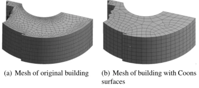
In this subsection the results of our algorithm will be explained using the model depicted in Figure 13 and Figure 14. After sep-arating the 280 polygons of the original model to 23 collections, and replacing six of these collections with Coons surfaces, our algorithm recreated a building model with a total of 23 surfaces. This simplification of the building model reduced the required memory by 90%. Figure 16 shows the mesh created for the origi-nal model (a) and the one created after using the Coons algorithm (b). Having applied the algorithm, the meshing tool did not have to use the thin edges of the polygons of the original building for orientation. As a result, we were able reduce the number of mesh elements by 80 percent for the processed model, while the aver-age aspect ratio got closer to one and therefore the quality of the mesh increased. For this example we used a rough mesh to make the difference obvious.
(a) Mesh of original building (b) Mesh of building with Coons surfaces
Figure 16. Comparison of meshes of(a)original building with arches represented by thin polygons and(b)building with arches
replaced by Coons surfaces
6. CONCLUSION
observed that many building elements were replaced by Coons surfaces without a deformation of the original shape. Using the Coons surfaces in city models produced satisfying results as one can see in Figure 16 in subsection 5.4. By replacing multiple small polygons, the model was greatly simplified and the required memory of the CAD model notably reduced. Furthermore, we were able to improve the quality of the derived finite element mesh. While many buildings could be processed using our rithm, we also found various complex buildings, where our algo-rithm could not be applied yet. In most cases this is traced back to the algorithm of Coons, which requires four boundary curves, that are not always given.
The automated simplification or generalization of LoD3 build-ings is challenging, as there is no general algorithm which works with every model. The simplification algorithm needs to be ad-justed due to differences in model and requirement. Thus, auto-mated model simplification of LoD3 buildings might not provide the expected or needed results, but it still helps to reduce manual processing for many models.
Nevertheless, there is still a lot more that can be done to advance in the field of simplification.
REFERENCES
Alam, N., Wagner, D., Wewetzer, M., von Falkenhausen, J., Coors, V. and Pries, M., 2013. Towards Automatic Validation and Healing of CityGML Models for Geometric and Semantic Consistency.ISPRS Annals of Photogrammetry, Remote Sensing and Spatial Information Sciences1(1), pp. 1–6.
Farin, G., 2014. Curves and surfaces for computer-aided geo-metric design: a practical guide. Elsevier.
Kolbe, T. H., 2009. Representing and exchanging 3D city mod-els with CityGML. In: 3D geo-information sciences, Springer, pp. 15–31.
Ma, W. and Kruth, J.-P., 1998. Nurbs curve and surface fitting for reverse engineering. The International Journal of Advanced Manufacturing Technology14(12), pp. 918–927.
Open Geospatial Consortium, 2012. OGC city geography markup language (CityGML) encoding standard V2. 0. OGC Doc.
Piegl, L. and Tiller, W., 2012. The NURBS book. Springer Sci-ence & Business Media.
Schilling, A., 2014. Integrated 3D City Models Support Blast / Evacuation Visualization for Critical Infrastructure in Urban En-vironments. 3D Visualization World feature article, published on 14 April 2014. http://3dvisworld.com.
SIG-3D Quality Working Group, 2012. Handbuch f¨ur die Model-lierung von 3D Objekten-Teil 2: ModelModel-lierung Geb¨aude (LOD1, LOD2 und LOD3).