Lagrangian analysis of microphysical and chemical processes in the Antarctic stratosphere: a case study

(1)

ACPD

14, 32629–32665, 2014

Lagrangian analysis of Antarctic stratosphere

L. Di Liberto et al.

Title Page

Abstract Introduction

Conclusions References

Tables Figures

◭ ◮

Back Close

Full Screen / Esc

Printer-friendly Version Interactive Discussion

Discussion

P

a

per

|

Discussion

P

a

per

|

Discussion

P

a

per

|

Discussion

P

a

per

Atmos. Chem. Phys. Discuss., 14, 32629–32665, 2014 www.atmos-chem-phys-discuss.net/14/32629/2014/ doi:10.5194/acpd-14-32629-2014

This discussion paper is/has been under review for the journal Atmospheric Chemistry and Physics (ACP). Please refer to the corresponding final paper in ACP if available.

Lagrangian analysis of microphysical and

chemical processes in the Antarctic

stratosphere: a case study

L. Di Liberto1, R. Lehmann2, I. Tritscher3,6, F. Fierli1, J. L. Mercer4, M. Snels1, G. Di Donfrancesco5, T. Deshler4, B. P. Luo3, J-U. Grooß6, E. Arnone1,

B. M. Dinelli1, and F. Cairo1

1

Institute for Atmospheric Sciences and Climate, ISAC-CNR, Italy 2

Alfred Wegener Institute, Potsdam, Germany 3

Institute for Atmospheric and Climate Science, ETH Zurich, Switzerland 4

Department of Atmospheric Science, University of Wyoming, Laramie, Wyoming, USA 5

Ente per le Nuove Tecnologie Energia e Ambiente, Santa Maria di Galeria, Rome, Italy 6

Institut für Energie und Klimaforschung – Stratosphäre (IEK-7), Forschungszentrum Jülich, Jülich, Germany

Received: 24 October 2014 – Accepted: 3 December 2014 – Published: 22 December 2014

Correspondence to: F. Cairo (f.cairo@isac.cnr.it)

(2)

ACPD

14, 32629–32665, 2014

Title Page

Tables Figures

◭ ◮

Back Close

Full Screen / Esc

Discussion

P

a

per

|

Discussion

P

a

per

|

Discussion

P

a

per

|

Discussion

P

a

per

|

Abstract

We investigated chemical and microphysical processes in the late winter in the Antarc-tic lower stratosphere, after the first chlorine activation and initial ozone depletion. We focused on a time interval when both further chlorine activation and ozone loss, but also chlorine deactivation, occur.

5

We performed a comprehensive Lagrangian analysis to simulate the evolution of an airmass along a ten-day trajectory, coupling a detailed microphysical box model with a chemistry model. Model results have been compared with in-situ and remote sensing measurements of particles and ozone at the start and end points of the trajectory, and satellite measurements of key chemical species and clouds along it.

10

Di_ﬀerent model runs have been performed to understand the relative role of solid and liquid Polar Stratospheric Cloud (PSC) particles for the heterogeneous chemistry, and for the denitrification caused by particle sedimentation. According to model results, under the conditions investigated, ozone depletion is not a_ﬀected significantly by the presence of Nitric Acid Trihydrate (NAT) particles, as the observed depletion rate can

15

equally well be reproduced by heterogeneous chemistry on cold liquid aerosol, with a surface area density close to background values.

Under the conditions investigated, the impact of denitrification is important for the abundances of chlorine reservoirs after PSC evaporation, thus stressing the need of using appropriate microphysical models in the simulation of chlorine deactivation.

Con-20

versely, we found that the eﬀect of particle sedimentation and denitrification on the amount of ozone depletion is rather small in the case investigated. In the first part of the analysed period, when a PSC was present in the airmass, sedimentation led to smaller available particle surface area and less chlorine activation, and thus less ozone depletion. After the PSC evaporation, in the last three days of the simulation,

25

(3)

ACPD

14, 32629–32665, 2014

Title Page

Tables Figures

◭ ◮

Back Close

Full Screen / Esc

Discussion

P

a

per

|

Discussion

P

a

per

|

Discussion

P

a

per

|

Discussion

P

a

per

1 Introduction

The depletion of ozone occurring in the polar stratosphere during winter and spring is linked to processes involving clouds in the polar stratosphere (Solomon et al., 1986). During winter the polar stratosphere cools to temperatures below 195 K, establishing a vortex circulation over the poles that separates the air inside from mid latitudes,

5

and allows for the formation of Polar Stratospheric Clouds (PSC). Such clouds can be classified into three main particle types (Browell et al., 1990; Toon et al., 1990), Ia as solid trihydrates of nitric acid (NAT), Ib as supercooled ternary solutions of H₂O/HNO₃/H₂SO₄ (STS) growing by HNO₃ uptake by pre-existing stratospheric sul-phate aerosol (SSA), type II as ice clouds, similar to tropospheric cirrus (Lowe et al.,

10

2008). A new classification by Pitts et al. (2007, 2009, 2011) emphasizes that PSCs are often composed of mixtures of such particle types. PSC classifications have been critically reviewed in Achtert et al. (2014).

Extensive observations from ground-based as well as satellite instruments have pro-vided climatologies of PSC occurrence in Antarctica (Adriani et al., 2004; Pitts et al.,

15

2007; Di Liberto et al., 2014) and in the Arctic (Maturilli et al., 2005). Antarctic PSCs, prevalently of type NAT, appear in early June to achieve maximum occurrence in July at 20–24 km. The altitude of maximum occurrence has a downward trend from 24 to 14 km between July and September. PSCs become increasingly rare to non-existent after the middle of October. Their presence is widespread over Antarctica, although regions of

20

enhanced occurrence are present above and eastward of the Antarctic Peninsula. Heterogeneous chemical reactions taking place on or within PSC particles convert relatively non-reactive chlorine reservoir species such as ClONO₂and HCl into active chlorine compounds as HOCl, ClNO₂ and Cl₂. Once the polar stratosphere has been primed by the action of heterogeneous chemistry on PSC particles, at the onset of

25

(4)

ACPD

14, 32629–32665, 2014

Title Page

Tables Figures

◭ ◮

Back Close

Full Screen / Esc

Discussion

P

a

per

|

Discussion

P

a

per

|

Discussion

P

a

per

|

Discussion

P

a

per

|

Sedimentation of large PSC particles containing water and nitric acid causes de-hydration and denitrification, depleting the stratosphere of water and nitric oxides that otherwise could reform chlorine reservoir species and reduce the lifetime of reactive chlorine. As the moderating eﬀect of NO_x is missing, the considerable buildup of ClO drives the successive decrease in stratospheric ozone (Solomon, 1999).

5

The various kinds of PSCs influence such processes differently: the conversion of chlorine from less to more reactive species takes place with different efficiency, related to di_fferent PSC types (Biele et al., 2001; Carslaw et al., 1997; Tsias et al., 1999; Weg-ner et al., 2012); moreover, the sedimentation rate strongly depends on the average PSC particle size, which depends on its composition, phase and formation process.

10

In this paper, a case study of PSC evolution and its impact on ozone depletion and related processes in the late winter Antarctic stratosphere is presented. The study is based on in-situ and remote sensing observations of trace gases and particles, and Lagrangian microphysical and chemical models. After a first observation of PSC opti-cal characteristics, particle size distributions and ozone taken over McMurdo Station

15

(77◦51′S, 166◦40′E) by a set of balloon-borne in-situ instruments and a ground based lidar, the airmass has been tracked with a trajectory model until, after ten days, air in a certain altitude range returned to McMurdo within a distance of less than 300 km. Then a second in-situ balloon sampling and lidar measurement was accomplished. Satellite measurements of key chemical species and particles along the airmass

tra-20

jectories documented its microphysical and chemical evolution. This dataset has been compared with simulations from chemical and microphysical box models reproducing the evolution of the cloud and evaluating its impact on the chemistry in the air mass. This well documented case took place in early September, soon after the onset of ozone depletion from chlorine activation but before complete destruction of ozone, in

25

(5)

impor-ACPD

14, 32629–32665, 2014

Title Page

Tables Figures

◭ ◮

Back Close

Full Screen / Esc

Discussion

P

a

per

|

Discussion

P

a

per

|

Discussion

P

a

per

|

Discussion

P

a

per

tance of the heterogeneous chemistry and denitrification will be made. The scope of this study is to provide a contribution to the most recent discussion of the relative role of PSC and liquid (background) aerosol in the ozone depletion (Drdla and Müller, 2012; Wegner et al., 2012; Wohltmann et al., 2013).

2 Instruments and Models 5

2.1 In-situ instruments

Balloon-borne instruments have been routinely launched from McMurdo Station since the 1980s (Mercer et al., 2007). Balloons are routinely equipped with instruments to measure ozone (Deshler et al., 2008), temperature, pressure and humidity, and oc-casionally with Optical Particle Counters (OPC) (Hofmann and Deshler, 1991; Adriani

10

et al., 1995; Deshler et al., 2003b).

Ozone measurements are performed with commercial electrochemical cell (ECC) ozonesondes, developed and described by Komhyr (1969). A Vaisala radio sonde RS92 performs pressure, temperature and humidity measurements using sensors de-signed to cover all atmospheric and weather conditions in every climate zone. The

15

model RS92 provides temperature and pressure with an accuracy respectively of 0.25 K and 0.2 hPa near 50 hPa (Steinbrecht et al., 2008).

The OPC counts and sizes particles drawn into a sampling chamber. The single parti-cle instrument uses white light scattering at 40◦_{in the forward direction to measure size}

using Mie theory. Deshler et al. (2003a) have described the measurement principles

20

(6)

ACPD

14, 32629–32665, 2014

Title Page

Tables Figures

◭ ◮

Back Close

Full Screen / Esc

Discussion

P

a

per

|

Discussion

P

a

per

|

Discussion

P

a

per

|

Discussion

P

a

per

|

2.2 Ground based lidar

McMurdo Station has been hosting a polarization diversity Rayleigh lidar since 1991 (Adriani et al., 2004), which was upgraded in 2004 (Di Liberto et al., 2014). The backscatter ratio, defined as the ratio of the total backscattered light to the one ex-pected from an atmosphere free of aerosol, is retrieved by using the Klett algorithm,

5

with an extinction-to backscatter ratio (lidar ratio) calculated using the empirical model proposed by Gobbi et al. (1995). The ratio of the parallel to the cross polarization signals, the volume depolarization ratioδ, is used to detect the presence of non spher-ical (i.e. solid) aerosol. This quantity is calibrated with the method described by Snels et al. (2009). The aerosol depolarization ratioδa, retrieved from δ by eliminating the

10

molecular contribution from the backscattering (Cairo et al., 1999), is a more direct characterization of the particle morphology, and is here presented. The uncertainty af-fecting these optical parameters has been estimated following the method reported in Russell et al. (1979) and is 0.1 (in absolute value) or 10 % of the measured value (the larger of the two) for the aerosol backscatter ratio (BR-1) and 3 % (in absolute value)

15

or 10 % of the measured value (the larger of the two) for the aerosol depolarization.

2.3 Satellite instruments

The Aura Microwave Limb Sounder (MLS) measures thermal emission continuously (24 h per day) using a limb viewing geometry which maximizes signal intensity and vertical resolution. Vertical profiles of mixing ratios of many diﬀerent chemical species,

20

temperature and pressure are derived (Waters et al., 2006). The MLS results for strato-spheric ozone have been extensively validated and are in good agreement with other datasets from many diﬀerent origins (Froidevaux et al., 2006). Ozone vertical profiles have vertical resolution of approximately 3 km from 215 to 0.2 hPa and about 4–6 km between 0.2 and 0.1 hPa. The ozone precision is 0.04 ppmv in the range 215–68 hPa,

25

(7)

ACPD

14, 32629–32665, 2014

Title Page

Tables Figures

◭ ◮

Back Close

Full Screen / Esc

Discussion

P

a

per

|

Discussion

P

a

per

|

Discussion

P

a

per

|

Discussion

P

a

per

estimated single-profile precision reported for the Level 2 product varies from 0.2 to 0.6 ppbv in the stratosphere. HNO₃ data are reliable over the range 215 to 3.2 hPa, with a vertical resolution of 3–4 km in the upper troposphere and lower stratosphere. The precision is approx. 0.6–0.7 ppbv throughout the range from 215 to 3.2 hPa (San-tee et al., 2007). Further information on the MLS instrumentation and its products can

5

be found at: http://mls.jpl.nasa.gov/.

In our study we have used MLS data in their version 2.2 generated by the GIOVANNI data analysis web application. We have considered MLS profiles when the MLS over-pass was included in a box of ±2◦ lat and ±15◦ lon with a time diﬀerence less than

12 h with respect to the airmass location along its trajectory. MLS data (delivered on

10

pressure levels) were interpolated to find the mixing ratio at the isentropic levels (or altitudes) of our interest. This has been done by identifying the pressure value at the isentrope (or altitude) of interest from our radiosoundings, then linearly interpolating the MLS data in term of logarithmic pressures.

MIPAS (Michelson Interferometer for Atmospheric limb Sounding) measured the

up-15

per tropospheric and stratospheric composition from a polar orbit on board the ESA ENVISAT satellite from 2002 to 2012 (Fisher et al., 2008). MIPAS was a limb-scanning Fourier Transform interferometer that measured emission spectra in the thermal in-frared, on a wide spectral range (680 to 2410 cm−1). We adopted MIPAS data from the MIPAS2D database (Dinelli et al., 2010), (http://www.isac.cnr.it/~rss/mipas2d.htm)

20

retrieved with the GMTR (Geo-fit Multi-Target Retrieval) analysis tool (Carlotti et al., 2006). The vertical resolution of MIPAS2D data is about 4 km for the altitude range of interest of this paper. Total systematic errors at the altitudes of interest for this study are: 3–8 % for pressure, 0.7–1.5 K for temperature, 5–7 % for ozone, and 5–20 % for the other species. Random errors are: 0.5–1.5 % for pressure, 0.2–0.3 K for temperature,

25

2–5 % for ozone, 2–10 % for the other species. We have considered MIPAS profiles when the overlap of the MIPAS overpass was included in a box of _±2◦ _{lat and}

±15◦

(8)

ACPD

14, 32629–32665, 2014

Title Page

Tables Figures

◭ ◮

Back Close

Full Screen / Esc

Discussion

P

a

per

|

Discussion

P

a

per

|

Discussion

P

a

per

|

Discussion

P

a

per

|

temperature, and the selected MIPAS2D profiles interpolated at the potential tempera-ture level of the models.

The Cloud-Aerosol Lidar with Orthogonal Polarization (CALIOP) is a two-wavelengths (532 and 1064 nm) lidar, with two polarizations at 532 nm, on board the CALIPSO (Cloud-Aerosol Lidar and Infrared Pathfinder Satellite Observation) satellite

5

which provides vertical profiles of aerosols and clouds, and has been extensively used for studies on PSC (Pitts et al., 2007, 2009, 2011). It has a vertical resolution between 30 and 60 m and a horizontal resolution of 333 m and 1 km for altitudes between 0.5 and 8.2 km and between 8.2 and 20.2 km, respectively. The CALIPSO satellite is part of the A-Train track (Stephens et al., 2002) and performs measurements on the same

10

MLS geo locations, only some few minutes later. In this work we considered CALIOP profiles collected during night time and matching the±1.0◦ latitude, ±2.5◦ longitude, ±6 h time diﬀerence criteria, with respect to the traced airmass location. More

informa-tion on CALIOP can be found at http://www-calipso.larc.nasa.gov/.

2.4 Trajectory model 15

During the field campaign, the air parcel trajectories were tracked by using the Goddard Space Flight Center (GSFC) isentropic trajectory model (http://acdb-ext.gsfc.nasa.gov/ Data_services/automailer/index.html). In the course of the data analysis, and for the purposes of this study, additional trajectory tools have been used for checking the re-sults of the field campaign. For the purpose of microphysical modelling, the air parcel

20

trajectories have been recalculated by the trajectory module of CLaMS (Chemical La-grangian Model of the Stratosphere) using 6 hourly ERA-Interim (Dee et al., 2011) wind and temperature fields with a horizontal resolution of 1◦×1◦. CLaMS is a modular

chem-istry transport model (CTM) system developed at Forschungszentrum Jülich, Germany (McKenna et al., 2002a, b; Konopka et al., 2004). Integration of trajectories has been

25

(9)

ACPD

14, 32629–32665, 2014

Title Page

Tables Figures

◭ ◮

Back Close

Full Screen / Esc

Discussion

P

a

per

|

Discussion

P

a

per

|

Discussion

P

a

per

|

Discussion

P

a

per

first PSC observation, starting on 10 September 2008 at 12:00 UTC. The vertical spac-ing between the trajectories is about 100 m in a vertical range between 350 and 450 K. The GSFC and CLaMS trajectories document similar paths travelled by the airmass, although wind speed was slightly lower during the first days of the simulation in the ERA Interim dataset.

5

2.5 Microphysical and optical model for PSC

The Zurich Optical and Microphysical box Model (ZOMM) has been developed for PSC simulations to study the formation, growth and evaporation of PSC particles determined by changes in temperature and pressure. ZOMM includes the following PSC formation pathways: Liquid background particles grow into STS droplets by uptake of HNO₃(Dye

10

et al., 1992; Carslaw et al., 1995). Ice nucleation takes place either homogeneously at su_ﬃciently low temperatures (Koop et al., 2000) or heterogeneously on the surfaces of foreign nuclei (Engel et al., 2013). NAT nucleation is implemented as heterogeneous nucleation on foreign nuclei (Hoyle et al., 2013) as well as on uncoated ice surfaces (Luo et al., 2003).

15

Small-scale temperature fluctuations, that are required to accurately reproduce ice number densities, are superimposed onto the synoptic-scale trajectories. The sedi-mentation of PSC particles is accounted for by using the column version of ZOMM as described in Engel et al. (2014). So far, ZOMM has always been initialized at typical background conditions for the winter polar stratosphere. This study required to

pre-20

scribe existing particle size distributions. We extracted those data from the OPC mea-surements taken at the trajectory starting points and complemented the condensed amount of H₂O and HNO₃with gas phase values measured by MLS. The optical out-put, calculated using Mie andT Matrix scattering codes (Mishchenko et al., 2012) can directly be compared to CALIOP measurements. The calculated surface area of PSCs

25

(10)

ACPD

14, 32629–32665, 2014

Title Page

Tables Figures

◭ ◮

Back Close

Full Screen / Esc

Discussion

P

a

per

|

Discussion

P

a

per

|

Discussion

P

a

per

|

Discussion

P

a

per

|

2.6 Chemistry model

The temporal evolution of the mixing ratios of chemical species along trajectories was simulated by the Alfred Wegener Institute chemical box model. It contains 48 chemi-cal species and 171 reactions, describing the stratospheric chemistry. It is based on a module for gas-phase chemistry described in Brasseur et al. (1997) and a module

5

for heterogeneous chemistry reported in Carslaw et al. (1995). Reaction rate constants have been updated to the values given by Sander (2011). For these simulations, the initial mixing ratios of ClO, HCl, HNO₃, CO, N₂O, H₂O, and O₃ were taken from the nearest MLS and ozonesonde measurements. The mixing ratios of NO_x(NO, NO₂) and ClONO₂ were assumed to be close to zero in agreement with the MIPAS ClONO₂

ob-10

servations. To start with balanced initial values, pre-runs of the chemical box model on a one day back-trajectory ending at the start point of the corresponding main trajectory were performed. The initial mixing ratios for these pre-runs were iteratively modified, until the MLS measurements were reproduced by the model at the end of the pre-run trajectory. Then the mixing ratios of all species at the end of the pre-run were used as

15

initial values for the run of the chemical box model on the main trajectory. As part of this procedure, a ClO_x (₌ClO₊2_·Cl₂O₂) mixing ratio consistent with the MLS ClO mea-surement was determined, which is essential for a correct simulation of the chemical ozone depletion.

3 Observations and simulations 20

3.1 McMurdo observations

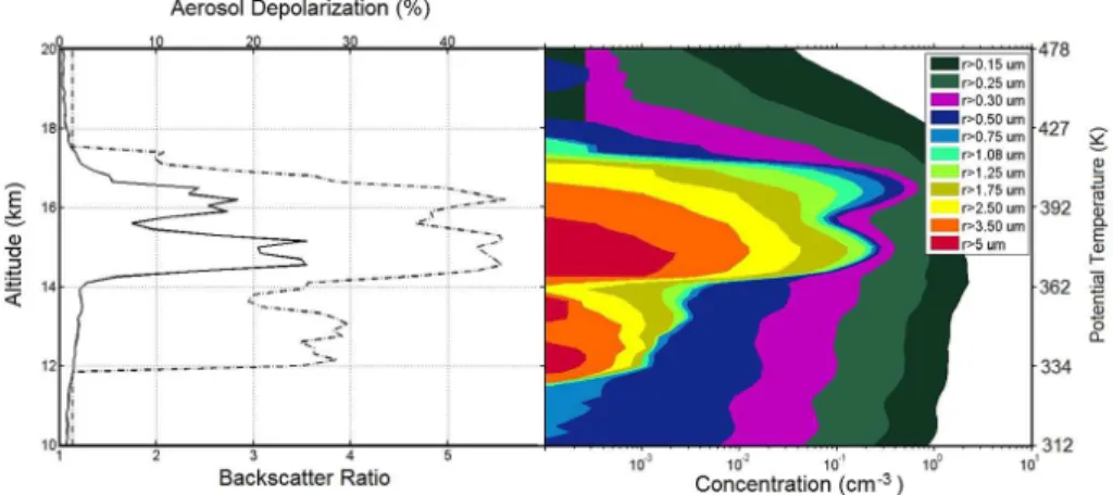
A balloon carrying an OPC and an ozone sonde was launched from the Antarctic sta-tion of McMurdo on 10 September 2008, 10:55 UTC. Lidar measurements were simul-taneously made during the 4 h duration of the balloon flight. The left panel of Fig. 1 depicts the lidar backscatter (solid line) and aerosol depolarization (dotted line) ratios

(11)

ACPD

14, 32629–32665, 2014

Title Page

Tables Figures

◭ ◮

Back Close

Full Screen / Esc

Discussion

P

a

per

|

Discussion

P

a

per

|

Discussion

P

a

per

|

Discussion

P

a

per

vs. altitude, averaged over the flight duration, while the right panel shows the particle size distribution measurements obtained by the OPC. A layered PSC can be clearly discerned between 11.5 and 17.5 km (approx. 330–420 K potential temperature). The lowermost layer shows small backscatter ratio values, but significant depolarization around 30 %, typical of NAT PSCs. The two layers between 14 (approx. 360 K) and

5

17 km show a higher backscatter ratio of about 3 and 2.5, depolarization around 40 %, again characteristic values for NAT PSCs. The particle size distribution confirms this classification, particles above 1 µm, typical of NAT particles (Voigt et al., 2000) reach-ing concentrations of up to 10−1cm−3. Temperatures (not shown) were above the ice freezing temperatureT_iceall along the profile.

10

Backtrajectory analysis showed that in the 10 days preceding the observation, the air in which the PSC was detected remained south of 60◦S, its temperature going below 195 K on 4 September, reaching 182 K the subsequent day and then howering around 190 K for the days prior to our observation.

The red solid line in Fig. 2 shows the measured ozone profile in the 300–500 K

po-15

tential temperature range, corresponding approximately to altitudes between 10 and 20 km. The ozone values on 10 September fall within the climatological variability re-ported in Kröger et al. (2003) at the onset of the mid-September ozone depletion. During the campaign, we tracked the airmass sampled by the in-situ instruments with the GSFC trajectory model finding that after approximately 10 days the air between 380

20

and 420 K potential temperature (where the PSC was observed) returned over the Ross Sea less than 300 km from McMurdo. A second balloon sounding was performed on 20 September 07:30 UTC, to match the return of the airmass close to the 400 K level. During this second balloon sounding, and in the 24 h preceding it, lidar measurements (not shown) showed no sign of PSCs. The ozone profile, in Fig. 2 with a blue solid

25

(12)

ACPD

14, 32629–32665, 2014

Title Page

Tables Figures

◭ ◮

Back Close

Full Screen / Esc

Discussion

P

a

per

|

Discussion

P

a

per

|

Discussion

P

a

per

|

Discussion

P

a

per

|

and 500 K (above 17 km up to 20 km). The gray area in Fig. 2 marks the altitude region where the airmass reencounter was expected. There, the two profiles show a similar depression with minima at 405 K. In that region, the ozone decrease between the two soundings is about 300 ppbv below 405 K, a little more above.

These ozone losses are comparable with what was observed in the past (Mercer

5

et al., 2007; Kröger et al., 2003; Nardi et al., 1999) in the same period of the year. The double overpass of the air mass over McMurdo in the layer between 380 and 420 K suggested a detailed Lagrangian study of the microphysics and chemistry that occurred in the air mass, between the two balloon observations.

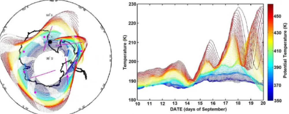
In the left panel of Fig. 3, isentropic air mass trajectories, starting from McMurdo on

10

10 September 2008 12:00 UTC are shown (color coded according to potential tempera-ture). Solid/dotted portions of the lines designate the sunlit/dark sectors of the trajecto-ries. The right panel reports temperature histories along those trajectories (again color coded in term of their potential temperature). The trajectories in the 375–425 K layer remained confined within the vortex and show a limited variability in PV (not shown).

15

Airmasses close to 400 K level returned over McMurdo after approximately 9.5 days. In those airmasses, the PSC was observed on 10 September and temperatures remained below 195 K for the initial five days of the trajectory. Then the airmasses experienced a warming in the second part of the trajectory.

To compare the results of our model simulations with observational data along the

20

path of the airmass, coincidences between the airmass trajectory and CALIOP and MLS observations were determined. In the leftmost panel of Fig. 3, purple dots indicate availability of MLS data, and purple lines crossing the trajectories specify intersections with CALIOP footprint.

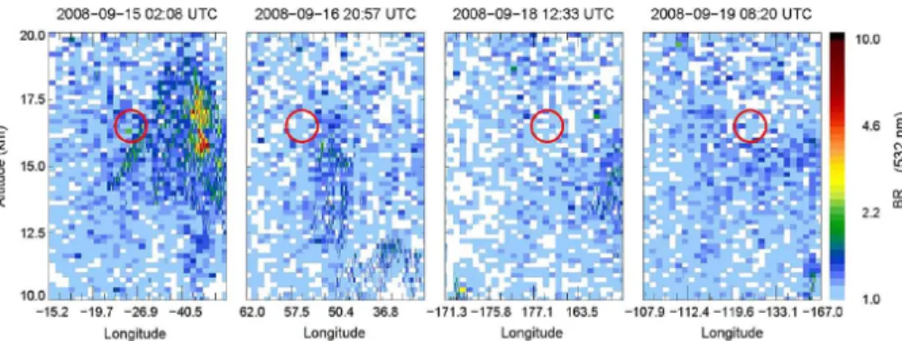
Figure 4 shows longitude vs. altitude curtains of backscatter ratio from CALIOP

25

(13)

pa-ACPD

14, 32629–32665, 2014

Title Page

Tables Figures

◭ ◮

Back Close

Full Screen / Esc

Discussion

P

a

per

|

Discussion

P

a

per

|

Discussion

P

a

per

|

Discussion

P

a

per

rameters which are the same order of magnitude of those observed above McMurdo four days earlier. On the next day, the top of a weak PSC is present in the region inter-sected by the air trajectory. Its shape resembles the previous day’s observations. On the night of 16 September the PSC is almost completely dissipated and vanishes in the following days. The CALIOP depolarization (not shown) indicates that observations are

5

consistent with a dominantly NAT PSC. The CALIOP observations document a large PSC in the area crossed by the trajectory of the airmass which was sampled five days earlier by the in-situ aerosol measurements from McMurdo.

3.2 Microphysical simulations

The microphysical model was initialized with MLS H₂O and HNO₃ profiles closest in

10

time and space to the first McMurdo balloon sounding. Since those values are gas phase values only, the amount of HNO₃ taken up by existing STS droplets and NAT particles at the time of the PSC observation had to be computed. For those calcula-tions we made use of the size distribution measured by the balloon-borne OPC. The smallest size bins up to 0.75 µm were considered to consist of STS droplets with a

den-15

sity of 1.44 g cm−3. Larger particles of the OPC size distribution were taken as NAT particles and the condensed HNO₃ phase was computed by assuming spherical NAT particles with a density of 1.62 g cm−3_{. Bimodal lognormal distributions fit to the PSC}

observations between 14.5 and 16 km indicated an average of 22 ppb HNO₃in the sec-ond (large particle) mode of the lognormal distribution. A possible overestimation of

20

HNO₃content in the condensed phase from particle size measurements was reported in some recent airborne measurements from the RECONCILE campaign (von Hobe et al., 2013) and possible reasons for that are extensively discussed in Molleker et al. (2014).

The microphysical run was initialized with an estimate of condensed HNO₃of 20 ppb,

25

(14)

tra-ACPD

14, 32629–32665, 2014

Title Page

Tables Figures

◭ ◮

Back Close

Full Screen / Esc

Discussion

P

a

per

|

Discussion

P

a

per

|

Discussion

P

a

per

|

Discussion

P

a

per

|

jectories. Temperature and pressure along the trajectories computed with the CLaMS trajectory module were used as input to predict the PSC evolution.

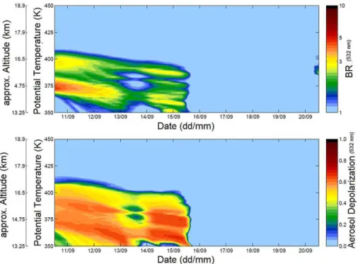
Figure 5 shows the modelled evolution of the PSC in terms of backscatter ratio (upper panel) and aerosol depolarization (lower panel) during the 10–20 September period. The persistence of the PSC for almost a week is evident. The cloud remains of NAT

5

type for 6 days after the first McMurdo balloon sounding, and totally evaporates three days before the second McMurdo sounding, as a warming caused its disappearance before 16 September. This warming in the second part of the trajectory coincides with an increasing distance of the airmass from the vortex centre. A vertical redistribution of the cloud is also evident, caused by the modelled particle sedimentation. The cloud

10

vertical extent changes from 410–360 K (approx. 17–14 km in geometrical altitude) to 390–350 K (approx. 16.5–13.5 km) in 6 days.

3.3 Chemical simulations

Chemistry model runs were performed along the CLaMS trajectories. Although the model has a microphysical module, it was forced to use prescribed values of HNO₃

15

(total and gas phase), STS/SSA and NAT aerosol surfaces, as provided oﬄine by the microphysical model output. This is because only the microphysical model could take into account particle sedimentation. The calculations were stopped at the trajectory point closest to McMurdo.

3.3.1 Effects of heterogeneous chemistry 20

Two model runs were performed, respectively with and without the inclusion of het-erogeneous chemistry. We hereafter present results of the simulations at the 400 K isentropic level, in the middle of the altitude region of the airmass trajectory match. As shown in Fig. 2, a trough in the ozone profile at 400 K implies that ozone depletion has markedly occurred already before the time of the first sounding. This isentropic

25

(15)

ACPD

14, 32629–32665, 2014

Title Page

Tables Figures

◭ ◮

Back Close

Full Screen / Esc

Discussion

P

a

per

|

Discussion

P

a

per

|

Discussion

P

a

per

|

Discussion

P

a

per

the consequences of particle sedimentation and HNO₃redistribution were likely to be more pronounced, as the microphysical simulation shows in Fig. 5, reporting profiles of backscatter ratio and aerosol depolarization. At 400 K, the NAT particle surface area decreased steadily from an initial value of 4.5 µm2cm−3 to 0 in 100 h, while STS/SSA particle surface area hovered around 1.5 µm2cm−3_{throughout the simulation, a value}

5

not far from what expected for the background aerosol surface area density (Hitchman et al., 1994; Chayka et al., 2008).

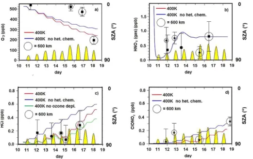
Figure 6 reports the results of the chemistry simulations, with (red line) and without (blue line) heterogeneous chemistry taken into account. Yellow regions represent sunlit parts of the trajectory. Figure 6a reports O₃evolution. Removing heterogeneous

reac-10

tions leads to less chlorine (re-)activation and, consequently, less ozone loss. However, the eﬀect is not very strong, because most of the chlorine is already activated at the beginning of the trajectory, according to MLS data. Squares represent ozone measured by MLS along the trajectory. There, and in the following panels, the radius of the circles surrounding the data points represents the match radius, defined as the distance

be-15

tween the observation and the location of the airmass on its trajectory, at the time of the observation. The simulations capture the integrated ozone loss well, although interme-diate comparisons are not good, as the large depletion is delayed in the observations until after 15 September. Such behaviour should not be expected in the present case, where both ClO_x and sunlight are available for ozone depletion throughout the whole

20

period. In the comparison with the measurements, however it has to be taken into ac-count that positions of the satellite measurements and corresponding trajectory points do usually not coincide. Moreover, limb soundings represent averages over large hori-zontal distances, and therefore might not have been able to fully account for processes going on in a relatively small portion of air.

25

(16)

ACPD

14, 32629–32665, 2014

Title Page

Tables Figures

◭ ◮

Back Close

Full Screen / Esc

Discussion

P

a

per

|

Discussion

P

a

per

|

Discussion

P

a

per

|

Discussion

P

a

per

|

sedimentation. Squares and stars represent respectively MLS and MIPAS data. In this case the agreement between simulation and observation seems reasonable although the measured uncertainties are large and the MIPAS and MLS scarcely agree with each other, with the MLS more consistent with the model. The microphysical model seems to well reproduce both the HNO₃ sequestering in condensed phase until 14

5

September, and then some denitrification. Note again that sedimentation processes are very localized and their eﬀects are observed by satellites only if the eﬀects cover a large area.

Heterogeneous chemistry aﬀects the evolution of HCl (Fig. 6c) and ClONO₂(Fig. 6d) respectively. As long as the PSC is present, both species are reduced by

heteroge-10

neous reactions. MLS HCl values are reported as squares and MIPAS ClONO₂ are reported as stars.

The comparison with the observed values seems to suggest that the simulation with heterogeneous chemistry active is more e_ﬀective in reproducing the HCl evolution over the studied period. However, as the speed of Cl deactivation is sensitively dependent

15

on ozone mixing ratios (Douglass et al., 1995; Grooß et al., 1997, 2011), but the ozone comparison is not fully satisfactory, it is di_ﬃcult to interpret this HCl and ClONO₂ com-parison. In order to estimate how sensitively HCl depends on the accuracy of ozone mixing ratio evolution in the present case, an additional sensitivity model run was then performed under the rather extreme assumption that there is no ozone depletion at all

20

(i.e. by holding constant the ozone mixing ratio to its initial value throughout the sim-ulation). Results of this sensitivity run are reported as a green solid line. The induced change in the HCl evolution is not too large, and HCl mixing ratios of the sensitivity run are still compatible with the MLS measurements between 12 and 17 September.

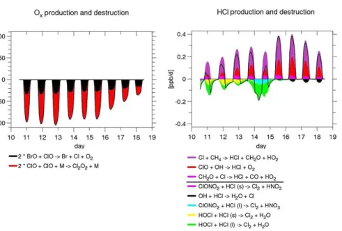
A closer look at the reactions aﬀecting ozone and HCl is presented in Fig. 7, reporting

25

(17)

ACPD

14, 32629–32665, 2014

Title Page

Tables Figures

◭ ◮

Back Close

Full Screen / Esc

Discussion

P

a

per

|

Discussion

P

a

per

|

Discussion

P

a

per

|

Discussion

P

a

per

of the chlorine activation is accomplished by the reaction of HCl with HOCl (both on NAT and STS/SSA), which is a result consistent with Grooß et al. (2011). There is a short time window (between 14 and 15 September) when also the reaction of HCl with ClONO₂ on STS/SSA is contributing. Before that period the ClONO₂ concentration is rather low, as reported in Fig. 6d, because most of the nitrogen is in NAT particles. After

5

that period the temperature is higher and thus the rate of the temperature-dependent reaction of ClONO₂ with HCl on liquid aerosol is smaller. In the model run, during the first days both NAT and liquid aerosol particles contribute to chlorine activation. After the sedimentation prevents further NAT particle existence, the reactions on liquid particles obviously prevail.

10

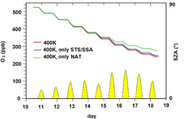
To further explore the relative role of NAT and STS/SSA, the model was run by separately switching on the heterogeneous reactions on NAT or on STS/SSA alone.

Figure 8 shows the O₃evolution with full heterogeneous chemistry (red), or with only heterogeneous chemistry on NAT (green) or on STS/SSA (blue). Although the hetero-geneous reactions on NAT particles contributed to the chlorine activation during the

15

first days (as shown in Fig. 6a), in our study STS/SSA particles might have been ef-fective on their own to produce the observed depletion occurred in 10 days after 10 September. Although a single case study does not allow to express any general state-ment for ozone depletion in the whole winter, our conclusion is in line with the results by Drdla and Müller (2012) (Arctic and Antarctic) and Wegner et al. (2012) and

Wohlt-20

mann et al. (2013) (Arctic), who argue that cold liquid aerosols alone could provide most of the chlorine activation. A major role of STS particles in driving the extreme ozone reduction in the Arctic 2011 was found by Arnone et al. (2012).

3.3.2 Effects of particle sedimentation

As the influence of PSCs on chemistry is twofold, providing the surface for

heteroge-25

(18)

ACPD

14, 32629–32665, 2014

Title Page

Tables Figures

◭ ◮

Back Close

Full Screen / Esc

Discussion

P

a

per

|

Discussion

P

a

per

|

Discussion

P

a

per

|

Discussion

P

a

per

|

constraints, obtained by performing a new run of the microphysical model that did not account for particle sedimentation. In such configuration, a PSC was produced be-tween 365 and 410 K, remaining in this vertical range for 5 days, before subsequent warming caused its evaporation.

Results of this model run are depicted in Fig. 9 which report the time evolution of

5

ClONO₂ (Fig. 9a), HCl (Fig. 9b) and O₃ (Fig. 9c). Red curves report simulations with sedimentation and blue curves report simulations with no sedimentation. The eﬀect of sedimentation (denitrification) is not very large, but still detectable. In the first phase, until 16 September when temperatures were low enough for the existence of the PSC, the lack of particle sedimentation in the microphysical model allowed NAT surfaces at

10

400 K to remain high, leading to enhanced chlorine activation, and enhanced ozone loss. After 15 September, the temperature became too high for NAT existence, signif-icantly decreasing the rates of the heterogeneous reactions on aerosols, and chlorine activation stopped. In absence of denitrification after PSC evaporation more chlorine is deactivated, the growth of HCl decreases by a factor 2, and similarly the buildup of

15

ClONO₂ increases by a factor 4, as more NO₂ is available so that, from the moment of PSC evaporation on, the absence of denitrification causes slightly less ozone deple-tion rates. The final amount of HCl is reduced with respect to the denitrified scenario, and that is the result of diﬀerent and counteracting eﬀects. During the PSC existence, more HCl is destroyed in heterogeneous reactions with HOCl and ClONO₂, as more

20

NAT surface is available. After the PSC evaporation, the ClO and OH mixing ratios are smaller in the not-denitrified scenario, because more NO₂ and HNO₃ are available to convert ClO_x and HO_x species to the reservoirs ClONO₂ and H₂O via the reaction of ClO and NO₂to produce ClONO₂, and OH with HNO₃to produce H₂O and NO₃. That is why the HCl production by the reaction of ClO with OH is reduced. A counteracting

25

(19)

ACPD

14, 32629–32665, 2014

Title Page

Tables Figures

◭ ◮

Back Close

Full Screen / Esc

Discussion

P

a

per

|

Discussion

P

a

per

|

Discussion

P

a

per

|

Discussion

P

a

per

4 Conclusions

An in-situ observation of an airmass when a PSC was present, by an optical particle counter and ozonometer on a balloon launched from the Antarctic station of McMurdo, where a polarization diversity lidar was also operating, provided information on PSC characteristics and ozone abundance. A trajectory analysis revealed that the air mass

5

at around the 400 K level was close to McMurdo Station ten days later, when lidar and ozone sounding were accomplished, showing a marked ozone depletion and no sign of PSCs. The McMurdo in-situ measurements were complemented by O₃, HCl, ClONO₂and HNO₃observations from the satellite-borne MLS and MIPAS instruments and by particle observation from the satellite-borne CALIOP lidar, taken along the air

10

mass trajectory connecting the two McMurdo overpass measurements. The observa-tions have been compared to microphysical and chemical box models, run along the air mass trajectory, to investigate the evolution of the PSC and the sensitivity of the modelled chemistry to its presence. The detailed microphysical box model reproduces the evolution and type of PSC, as documented by the CALIOP observations along the

15

airmass trajectory. The magnitude of ozone depletion was well captured by the chem-ical model, as were the evolution of the reservoir species HCl and ClONO₂. In our case study, ozone destruction processes were investigated at a time when there was already a significant amount of activated chlorine at the beginning of the simulations, and there was ozone depletion already before the time window analysed. This probably

20

explains why, in this case, along the trajectory investigated the eﬀect of heterogeneous chemistry on ozone depletion was not very large, accounting for a diﬀerence of less than 8 ppb day−1_{in the overall modeled ozone depletion rate of 35 ppb day}−1_{. As long}

as a NAT PSC existed (i.e. in the first half of the time interval investigated), it con-tributed to the chlorine activation. However, according to our findings, under the

condi-25

(20)

ACPD

14, 32629–32665, 2014

Title Page

Tables Figures

◭ ◮

Back Close

Full Screen / Esc

Discussion

P

a

per

|

Discussion

P

a

per

|

Discussion

P

a

per

|

Discussion

P

a

per

|

findings supports the view that additional surface area provided by solid PSC particles does not increase appreciably the chlorine activation, since in cold conditions the acti-vation could originate from heterogeneous chemistry on surfaces basically provided by a background aerosol distribution. As expected, diﬀerences arising from the presence of particles (whether background aerosol or PSC) and from heterogeneous chemistry

5

that they allow, are more remarkable when gas phase chlorine reservoirs are exam-ined. In fact, the buildup of HCl and, particularly, of ClONO₂is significantly reduced by heterogeneous reactions. Turning our attention to the e_ffect of denitrification on ozone depletion at 400 K, at the top of the observed PSC, we came to the conclusion that, in our study, this effect is small. In this case this may be due to two opposite effects

10

of denitrification (and the length of the time sub-intervals in which either of these ef-fects is dominant): (1) a reduction of the NAT surface area density and thus of their contribution to chlorine activation, and consequently of the ozone loss during the first 5 days of the simulation; (2) a counteracting reduction of chlorine deactivation and thus an increase of the ozone loss during the last 3 days of the simulation. Moreover, as will

15

be discussed later, the eﬀects of denitrification on HCl and ClONO₂ are opposite, so they cancel to some extent. Furthermore, the time interval that we investigate is such that in the “with denitrification” case the ozone depletion is still going on at the end of it, suggesting that the diﬀerence between the cases “with denitrification” and “without denitrification” might increase after the time interval we studied. In absence of

denitrifi-20

cation the HCl concentration decreases by a factor 2 after PSC evaporation, while the buildup of ClONO₂even quadrupled, showing how crucially the time taken for chlorine deactivation depends on HNO₃ redistribution due to the gravitational settling of NAT particles.

Summarizing, state-of-the-art microphysical and chemical models are able to

simu-25

(21)

ACPD

14, 32629–32665, 2014

Title Page

Tables Figures

◭ ◮

Back Close

Full Screen / Esc

Discussion

P

a

per

|

Discussion

P

a

per

|

Discussion

P

a

per

|

Discussion

P

a

per

chemistry on NAT and STS/SSA aerosol and of denitrification on the observed ozone depletion and chlorine partitioning. Under the investigated conditions, NAT PSC pres-ence is of little eﬀectiveness in promoting additional ozone depletion, in comparison with what might be already occurring on background aerosols alone at low tempera-tures. In our case study, although the influence of denitrification was significant, but of

5

opposite signs, on ClONO₂ and HCl abundances, its impact on ozone depletion was small.

Acknowledgements. The authors acknowledge the Programma Nazionale di Ricerca in Antar-tide (PNRA) and the Progetto Congiunto di Ricerche CNR-CNRS STRACLIMA for financial support, and the National Science Foundation (NSF) for logistics and technical support on the

10

site. Jennifer Mercer and Terry Deshler were supported by the NSF under, most recently, OPP Grant 0839124. This work was also partially funded by the European Commission under the grant number RECONCILE-226365-FP7-ENV-2008-1.

References

Achtert, P. and Tesche, M.: Assessing lidar-based classification schemes for polar stratospheric

15

clouds based on 16 years of measurements at Esrange, Sweden, J. Geophys. Res., 119, 1386–1405, 2014. 32631

Adriani, A., Deshler, T., Di Donfrancesco, G., and Gobbi, G. P.: Polar stratospheric clouds and volcanic aerosol during 1992 spring over McMurdo Station, Antarctica: lidar and particle counter comparisons, J. Geophys. Res., 100, 25877–25898, 1995. 32633

20

Adriani, A., Massoli, P., Di Donfrancesco, G., Cairo, F., Moriconi, M. L., and Snels, M.: Cli-matology of polar stratospheric clouds based on lidar observations from 1993 to 2001 over McMurdo Station, Antarctica, J. Geophys. Res., 109, D24211, doi:10.1029/2004JD004800, 2004. 32631, 32634

Arnone, E., Castelli, E., Papandrea, E., Carlotti, M., and Dinelli, B. M.: Extreme ozone depletion

25

(22)

ACPD

14, 32629–32665, 2014

Title Page

Tables Figures

◭ ◮

Back Close

Full Screen / Esc

Discussion

P

a

per

|

Discussion

P

a

per

|

Discussion

P

a

per

|

Discussion

P

a

per

|

Biele, J., Tsias, A., Luo, B. P., Carslaw, K. S., Neuber, R., Beyerle, G., and Peter, T.: Nonequi-librium coexistence of solid and liquid particles in Arctic stratospheric clouds, J. Geophys. Res., 106, 22991–23007, doi:10.1029/2001JD900188, 2001. 32632

Brasseur, G. P., Tie, X. X., Rasch, P. J., and Lefèvre, F.: A three-dimensional simulation of the Antarctic ozone hole: Impact of anthropogenic chlorine on the lower stratosphere and upper

5

troposphere, J. Geophys. Res., 102, 8909–8930, 1997. 32638

Browell, E. V., Butler, C. F., Ismail, S., Robinette, P. A., Carter, A. F., Higdon, N. S., Toon, O. B., Shoeberl, M. R., and Tuck, A. F.: Airborne lidar observations in the wintertime Arctic strato-sphere: polar stratospheric clouds, Geophys. Res. Lett., 17, 385–388, 1990. 32631

Cairo, F., Di Donfrancesco, G., Adriani, A., Pulvirenti, L., and Fierli, F.: Comparison of various

10

linear depolarization parameters measured by lidar, Appl. Optics, 38, 4425–4432, 1999. Carlotti, M., Brizzi, G., Papandrea, E., Prevedelli, M., Ridolfi, M., Dinelli, B. M., and Magnani, L.:

GMTR: two-dimensional geo-fit multitarget retrieval model for Michelson Interferometer for Passive Atmospheric Sounding/Environmental Satellite observations, Appl. Optics, 45, 716– 727, doi:10.1364/AO.45.000716, 2006. 32635

15

Carslaw, K. S. and Peter, T.: Uncertainties in reactive uptake coeﬃcients for solid stratospheric particles – 1. Surface chemistry, Geophys. Res. Lett., 24, 1743–1746, 1997. 32632

Carslaw, K. S., Luo, B. P., and Peter, T.: An analytic expression for the composition of aqueous HNO3-H2SO4 stratospheric aerosols including gas phase removal of HNO3, Geophys. Res. Lett., 22, 1877–1880, 1995. 32637, 32638

20

Chayka, A. M., Timofeyev, Y. M., and Polyakov, A. V.: Integral microphysical parameters of stratospheric background aerosol for 2002–2005 (the SAGE III Satellite Experiment), Izv. Atmos. Ocean. Phy., 44, 206–220, 2008. 32643

Dee, D. P., Uppala, S. M., Simmons, A. J., Berrisford, P., Poli, P., Kobayashi, S., Andrae, U., Balmaseda, M. A., Balsamo, G., Bauer, P., Bechtold, P., Beljaars, A. C. M., van de Berg, L.,

25

Bidlot, J., Bormann, N., Delsol, C., Dragani, R., Fuentes, M., Geer, A. J., Haimberger, L., Healy, S. B., Hersbach, H., Hólm, E. V., Isaksen, L., Kållberg, P., Köhler, M., Matricardi, M., McNally, A. P., Monge-Sanz, B. M., Morcrette, J.-J., Park, B.-K., Peubey, C., de Rosnay, P., Tavolato, C., Thépaut, J.-N., and Vitart, F.: The ERA-Interim reanalysis: configuration and performance of the data assimilation system, Q. J. Roy. Meteor. Soc., 137, 553–597,

30

doi:10.1002/qj.828, 2011. 32636

(23)

ACPD

14, 32629–32665, 2014

Title Page

Tables Figures

◭ ◮

Back Close

Full Screen / Esc

Discussion

P

a

per

|

Discussion

P

a

per

|

Discussion

P

a

per

|

Discussion

P

a

per

using balloon-borne instruments, J. Geophys. Res., 108, 4167, doi:10.1029/2002JD002514, 2003a. 32633

Deshler, T., Larsen, N., Weisser, C., Schreiner, J., Mauersberger, K., Cairo, F., Adriani, A., Di Donfrancesco, G., Ovarlez, J., Ovarlez, H., Blum, U., Fricke, K. H., and Dörnbrack, A.:, Large nitric acid particles at the top of an Arctic stratospheric cloud, J. Geophys. Res., 108,

5

4517, doi:10.1029/2003JD003479, 2003b. 32633

Deshler, T., Mercer, J. M.,. Smit, H. G. J, Stubi, R., Levrat, G., Johnson, B. J., Oltmans, S. J., Kivi, R., Thompson, A. M., Witte, J., Davies, J., Schmidlin, F. J., Brothers, G., and Sasaki, T.: Atmospheric comparison of electrochemical cell ozonesondes from diﬀerent manufactur-ers, and with diﬀerent cathode solution strengths: the Balloon Experiment on standards for

10

ozonesondes, J. Geophys. Res., 113, D04307, doi:10.1029/2007JD008975, 2008. 32633 Di Liberto, L., Cairo, F., Fierli, F., Di Donfrancesco, G., Viterbini, M., Deshler, T., and

Snels, M.: Observation of polar stratospheric clouds over McMurdo (77.85◦_{S, 166.67}◦_E) (2006–2010), J. Geophys. Res.-Atmos., 119, 5528–5541, doi:10.1002/2013JD019892, 2014. 32631, 32634

15

Dinelli, B. M., Arnone, E., Brizzi, G., Carlotti, M., Castelli, E., Magnani, L., Papandrea, E., Prevedelli, M., and Ridolfi, M.: The MIPAS2D database of MIPAS/ENVISAT measurements retrieved with a multi-target 2-dimensional tomographic approach, Atmos. Meas. Tech., 3, 355–374, doi:10.5194/amt-3-355-2010, 2010. 32635

Douglass, A. R., Schoeberl, M. R., Stolarski, R. S., Waters, J. W., Russell, J. M., Roche, A. E.,

20

and Massie, S. T.: Interhemispheric diﬀerences in springtime production of HCl and ClONO2 in the polar vortices, J. Geophys. Res., 100, 13967–13978, 1995. 32644

Drdla, K., and Müller, R.: Temperature thresholds for chlorine activation and ozone loss in the polar stratosphere, Ann. Geophys., 30, 1055–1073, doi:10.5194/angeo-30-1055-2012, 2012. 32633, 32645

25

Dye, J. E., Baumgardner, D., Gandrud, B. W., Kawa, S. R., Kelly, K. K., Loewenstein, M., Ferry, G. V., Chan, K. R., and Gary, B. L.: Particle size distributions in Arctic polar strato-spheric clouds, growth and freezing of sulfuric acid droplets, and implications for cloud for-mation, J. Geophys. Res., 97, 8015–8034, doi:10.1029/91JD02740, 1992. 32637

Engel, I., Luo, B. P., Pitts, M. C., Poole, L. R., Hoyle, C. R., Grooß, J.-U., Dörnbrack, A., and

30

(24)

ACPD

14, 32629–32665, 2014

Title Page

Tables Figures

◭ ◮

Back Close

Full Screen / Esc

Discussion

P

a

per

|

Discussion

P

a

per

|

Discussion

P

a

per

|

Discussion

P

a

per

|

Engel, I., Luo, B. P., Khaykin, S. M., Wienhold, F. G., Vömel, H., Kivi, R., Hoyle, C. R., Grooß, J.-U., Pitts, M. C., and Peter, T.: Arctic stratospheric dehydration – Part 2: Microphysical mod-eling, Atmos. Chem. Phys., 14, 3231–3246, doi:10.5194/acp-14-3231-2014, 2014. 32637 Fischer, H., Birk, M., Blom, C., Carli, B., Carlotti, M., von Clarmann, T., Delbouille, L.,

Dud-hia, A., Ehhalt, D., Endemann, M., Flaud, J. M., Gessner, R., Kleinert, A., Koopman, R.,

5

Langen, J., López-Puertas, M., Mosner, P., Nett, H., Oelhaf, H., Perron, G., Remedios, J., Ridolfi, M., Stiller, G., and Zander, R.: MIPAS: an instrument for atmospheric and climate research, Atmos. Chem. Phys., 8, 2151–2188, doi:10.5194/acp-8-2151-2008, 2008. 32635 Froidevaux, L., Livesey, N. J., Read, W. G., Jiang, Y. B., Jimenez, C, Filipiak, M. J.,

Schwartz, M. J., Santee, M. L., Pumphrey, H. C., Jiang, J. H., Wu, D. L., Manney, G. L.,

10

Drouin, B. J., Waters, J. W., Fetzer, E. J., Bernath, P. F., Boone, C. D., Walker, K. A., Jucks, K. W., Toon, G. C., Margitan, J. J., Sen, B., Webster, C. R., Christensen, L. E., Elkins, J. W., Atlas, E., Lueb, R. A., and Hendershot, R.: Early validation analyses of at-mospheric profiles from EOS MLS on the Aura Satellite, IEEE T. Geosci. Remote, 44, 1106– 1121, 2006. 32634

15

Gobbi, G. P.: Lidar estimation of stratospheric aerosol properties: surface, volume, and extinc-tion to backscatter ratio, J. Geophys. Res., 100, 11219–11235, 1995. 32634

Grooß, J. U., Pierce, R. B., Crutzen, P. J., Grose, W. L., and Russell, J. M.: Re-formation of chlorine reservoirs in Southern Hemisphere polar spring, J. Geophys. Res., 102, 13141– 13152, 1997. 32644

20

Grooß, J.-U., Brautzsch, K., Pommrich, R., Solomon, S., and Müller, R.: Stratospheric ozone chemistry in the Antarctic: what determines the lowest ozone values reached and their re-covery?, Atmos. Chem. Phys., 11, 12217–12226, doi:10.5194/acp-11-12217-2011, 2011. 32644, 32645

Hitchman, M. H., McKay, M., and Trepte, C. R.: A climatology of stratospheric aerosol, J.

Geo-25

phys. Res., 99, 20689–20700, 1994. 32643

Hofmann, D. J. and Deshler, T.: Stratospheric cloud observations during formation of the Antarc-tic ozone hole in 1989, J. Geophys. Res., 96, 2897–2912, 1991. 32633

Hoyle, C. R., Engel, I., Luo, B. P., Pitts, M. C., Poole, L. R., Grooß, J.-U., and Peter, T.: Hetero-geneous formation of polar stratospheric clouds – Part 1: Nucleation of nitric acid trihydrate

30

(NAT), Atmos. Chem. Phys., 13, 9577–9595, doi:10.5194/acp-13-9577-2013, 2013. 32637 Komhyr, W. D.: Electrochemical concentration cells for gas analysis, Ann. Geophys.-Italy, 25,

(25)

ACPD

14, 32629–32665, 2014

Title Page

Tables Figures

◭ ◮

Back Close

Full Screen / Esc

Discussion

P

a

per

|

Discussion

P

a

per

|

Discussion

P

a

per

|

Discussion

P

a

per

Konopka, P., Steinhorst, H. M., Grooß, J. U., Günther, G., Müller, R., Elkins, J. W., Jost, H. J., Richard, E., Schmidt, U., Toon, G., and McKenna, D. S.: Mixing and ozone loss in the 1999– 2000 Arctic vortex: simulations with the three-dimensional Chemical Lagrangian Model of the Stratosphere (CLaMS), J. Geophys. Res., 109, D02315, doi:10.1029/2003JD003792, 2004. 32636

5

Koop, T., Luo, B. P., Tsias, A., and Peter, T.: Water activity as the determinant for homogeneous ice nucleation in aqueous solutions, Nature, 406, 611–614, doi:10.1038/35020537, 2000. 32637

Kröger, C., Hervig, M., Nardi, B., Oolman, L., Deshler, T., Wood, S., and Nichol, S.: Strato-spheric ozone reaches new minima above McMurdo Station, Antarctica, between 1998 and

10

2001, J. Geophys. Res., 108, 4555–4567, doi:10.1029/2002JD002904, 2003. 32639, 32640 Lowe, D. and MacKenzie, A. R.: Polar stratospheric cloud microphysics and chemistry, J. Atmos.

Sol.-Terr. Phy., 70, 13–40, 2008. 32631

Nardi, B., Bellon, W., Oolman, L. D., and Deshler, T.: Spring 1996 and 1997 ozonesonde measurements over McMurdo Station, Antarctica, Geophys. Res. Lett., 22, 723–726, 1999.

15

32640

Luo, B. P., Voigt, C., Fueglistaler, S., and Peter, T.: Extreme NAT supersaturations in mountain wave ice PSCs: a clue to NAT formation, J. Geophys. Res., 108, 4441, doi:10.1029/2002JD003104, 2003. 32637

Maturilli, M., Neuber, R., Massoli, P., Cairo, F., Adriani, A., Moriconi, M. L., and Di

Don-20

francesco, G.: Diﬀerences in Arctic and Antarctic PSC occurrence as observed by lidar in Ny-Ålesund (79◦_{N, 12}◦_{E) and McMurdo (78}◦_{S, 167}◦_{E), Atmos. Chem. Phys., 5, 2081–2090,} doi:10.5194/acp-5-2081-2005, 2005. 32631

McKenna, D. S., Konopka, P., Grooß, J.-U., Günther, G., Müller, R., Spang, R., Oﬀ er-man, D., and Orsolini, Y.: A new Chemical Lagrangian Model of the Stratosphere (ClaMS):

25

1. Formulation of advection and mixing, J. Geophys. Res., 107, ACH 15-1–ACH 15-15, doi:10.1029/2000JD000114, 2002a. 32636

McKenna, D. S., Grooß, J.-U., Günther, G., Konopka, P., Müller, R., Carver, G., and Sasano, Y.: A new Chemical Lagrangian Model of the Stratosphere (CLaMS): 2. Formu-lation of chemistry scheme and initialization, J. Geophys. Res., 107, ACH 4-1–ACH 4-14,

30

doi:10.1029/2000JD000113, 2002b. 32636

(26)

Mc-ACPD

14, 32629–32665, 2014

Title Page

Tables Figures

◭ ◮

Back Close

Full Screen / Esc

Discussion

P

a

per

|

Discussion

P

a

per

|

Discussion

P

a

per

|

Discussion

P

a

per

|

Murdo Station, Antarctica, 1989–2003, during austral winter/spring, J. Geophys. Res., 112, D19307, doi:10.1029/2006JD007982, 2007. 32633, 32640

Mishchenko, M. I., Travis, L. D., and Mackowski, D. W.: T-matrix computations of light scat-tering by nonspherical particles: a review, J. Quant. Spectrosc. Ra., 111, 1704–1744, doi:10.1016/0022-4073(96)00002-7, 2010. 32637

5

Molleker, S., Borrmann, S., Schlager, H., Luo, B., Frey, W., Klingebiel, M., Weigel, R., Ebert, M., Mitev, V., Matthey, R., Woiwode, W., Oelhaf, H., Dörnbrack, A., Stratmann, G., Grooß, J.-U., Günther, G., Vogel, B., Müller, R., Krämer, M., Meyer, J., and Cairo, F.: Microphysical prop-erties of synoptic-scale polar stratospheric clouds: in situ measurements of unexpectedly large HNO3-containing particles in the Arctic vortex, Atmos. Chem. Phys., 14, 10785–10801,

10

doi:10.5194/acp-14-10785-2014, 2014. 32641

Nardi, B., Bellon, W., Oolman, L. D., and Deshler, T.: Spring 1996 and 1997 ozonesonde mea-surements over McMurdo Station, Antarctica, Geophys. Res. Lett., 26, 723–726, 1999. Pitts, M. C., Thomason, L. W., Poole, L. R., and Winker, D. M.: Characterization of Polar

Strato-spheric Clouds with spaceborne lidar: CALIPSO and the 2006 Antarctic season, Atmos.

15

Chem. Phys., 7, 5207–5228, doi:10.5194/acp-7-5207-2007, 2007. 32631, 32636

Pitts, M. C., Poole, L. R., and Thomason, L. W.: CALIPSO polar stratospheric cloud observa-tions: second-generation detection algorithm and composition discrimination, Atmos. Chem. Phys., 9, 7577–7589, doi:10.5194/acp-9-7577-2009, 2009. 32631, 32636

Pitts, M. C., Poole, L. R., Dörnbrack, A., and Thomason, L. W.: The 2009–2010 Arctic polar

20

stratospheric cloud season: a CALIPSO perspective, Atmos. Chem. Phys., 11, 2161–2177, doi:10.5194/acp-11-2161-2011, 2011. 32631, 32636

Plöger, F., Konopka, P., Günther, G., Grooß, J.-U., and Müller, R.: Impact of the vertical veloc-ity scheme on modeling transport in the tropical tropopause layer, J. Geophys. Res., 115, D03301, doi:10.1029/2009JD012023, 2010. 32636

25

Russell, P. B., Swissler, T. J., and McCormick, M. P.: Methodology for error analysis and simu-lation of lidar aerosol measurements, Appl. Optics, 18, 3783–3797, 1979. 32634

Sander, S. P.S, Friedl, R. R., Barker, J. R., Golden, D. M., Kurylo, M. J., Wine, P. H., Ab-batt, J. P. D., Burkholder, J. B., Kolb, C. E., Moortgat, G. K., Huie, R. E., and Orkin, V. L.: Chemical kinetics and photochemical data for use in atmospheric studies, Evaluation

Num-30