Uncertainties in modeling heterogeneous chemistry and Arctic ozone depletion in the winter 2009/2010

(1)

ACPD

12, 26245–26295, 2012

Uncertainties in modeling ozone

depletion

I. Wohltmann et al.

Title Page

Abstract Introduction

Conclusions References

Tables Figures

◭ ◮

Back Close

Full Screen / Esc

Printer-friendly Version Interactive Discussion

Discussion

P

a

per

|

Dis

cussion

P

a

per

|

Discussion

P

a

per

|

Discussio

n

P

a

per

|

Atmos. Chem. Phys. Discuss., 12, 26245–26295, 2012 www.atmos-chem-phys-discuss.net/12/26245/2012/ doi:10.5194/acpd-12-26245-2012

Atmospheric Chemistry and Physics Discussions

This discussion paper is/has been under review for the journal Atmospheric Chemistry and Physics (ACP). Please refer to the corresponding final paper in ACP if available.

Uncertainties in modeling heterogeneous

chemistry and Arctic ozone depletion in

the winter 2009/2010

I. Wohltmann1, T. Wegner2, R. M ¨uller2, R. Lehmann1, M. Rex1, G. L. Manney3,4,

M. L. Santee5, P. Bernath6,7, O. Sumi ´nska-Ebersoldt8, F. Stroh2, M. von Hobe2,

C. M. Volk9, E. H ¨osen9, F. Ravegnani10, A. Ulanovsky11, and V. Yushkov11

1

Alfred Wegener Institute for Polar and Marine Research, Potsdam, Germany

2

Institute of Energy and Climate Research – Stratosphere (IEK-7), Forschungszentrum J ¨ulich, J ¨ulich, Germany

3

NorthWest Research Associates, Inc., Socorro, New Mexico, USA

4

New Mexico Institute of Mining and Technology, Socorro, New Mexico, USA

5

Jet Propulsion Laboratory, California Institute of Technology, Pasadena, California, USA

6

University of York, York, UK

7

Old Dominion University, Norfolk, VA, USA

8

Institute of Meteorology and Climate Research, Karlsruhe Institute of Technology, Karlsruhe, Germany

9

University of Wuppertal, Department of Physics, Wuppertal, Germany

10

ISAC-CNR, Bologna, Italy

11

(2)

ACPD

12, 26245–26295, 2012

depletion

I. Wohltmann et al.

Title Page

Tables Figures

◭ ◮

Back Close

Full Screen / Esc

Discussion

P

a

per

|

Dis

cussion

P

a

per

|

Discussion

P

a

per

|

Discussio

n

P

a

per

|

Received: 13 September 2012 – Accepted: 19 September 2012 – Published: 5 October 2012

Correspondence to: I. Wohltmann ([email protected])

(3)

ACPD

12, 26245–26295, 2012

depletion

I. Wohltmann et al.

Title Page

Tables Figures

◭ ◮

Back Close

Full Screen / Esc

Discussion

P

a

per

|

Dis

cussion

P

a

per

|

Discussion

P

a

per

|

Discussio

n

P

a

per

|

Abstract

Stratospheric chemistry and denitrification are simulated for the Arctic winter 2009/2010 with the Lagrangian Chemistry and Transport Model ATLAS. A number of sensitivity runs is used to explore the impact of uncertainties in chlorine activation and denitrification on the model results. In particular, the e_fficiency of chlorine activation on

5

different types of liquid aerosol versus activation on nitric acid trihydrate clouds is ex-amined. Additionally, the impact of changes in reaction rate coefficients, in the particle number density of polar stratospheric clouds, in supersaturation, temperature or the ex-tent of denitrification is investigated. Results are compared to satellite measurements of MLS and ACE-FTS and to in-situ measurements onboard the Geophysica aircraft

10

during the RECONCILE measurement campaign. It is shown that even large changes in the underlying assumptions have only a small impact on the modeled ozone loss, even though they can cause considerable differences in chemical evolution and den-itrification. In addition, it is shown that chlorine activation on liquid aerosols alone is able to explain the observed magnitude and morphology of the mixing ratios of active

15

chlorine, reservoir gases and ozone.

1 Introduction

After the discovery of the Antarctic ozone hole (Farman et al., 1985), the rapid de-velopment of a robust theory of anthropogenic ozone depletion was a great scientific achievement. Since then, many aspects of this theory have been confirmed in a great

20

number of modeling and observational studies (e.g. Solomon, 1999; WMO, 2011). However, uncertainties in theory and observations of polar ozone depletion and limita-tions in modeling the complex processes in Chemistry and Transport Models (CTMs) remain an important issue. This is especially true for the microphysics and chemistry of Polar Stratospheric Clouds (PSCs) (e.g. Lowe and MacKenzie, 2008; Peter and Grooß,

25

(4)

ACPD

12, 26245–26295, 2012

depletion

I. Wohltmann et al.

Title Page

Tables Figures

◭ ◮

Back Close

Full Screen / Esc

Discussion

P

a

per

|

Dis

cussion

P

a

per

|

Discussion

P

a

per

|

Discussio

n

P

a

per

|

– In 2005, K. Drdla attracted attention with her hypothesis that the generally ac-cepted mechanism of dominant chlorine activation on clouds composed of nitric acid trihydrate (NAT) or supercooled ternary solutions (STS) might not be nec-essary for efficient chlorine activation and that heterogeneous activation of chlo-rine reservoir species might very efficiently occur already on the cold background

5

aerosol (e.g. Drdla, 2005; Drdla and M ¨uller, 2012). In fact, it is largely unknown to what extent liquid aerosols contribute to chlorine activation in relation to NAT clouds in the atmosphere. A change in this ratio would have important implications for the prediction of future ozone depletion in model scenarios. Drdla’s hypothesis is backed by the current low estimates of NAT number density, the required high

10

supersaturation of HNO₃ over NAT and the large uncertainties in reaction rates on NAT, which we will discuss in detail later.

– Reaction rate coefficients on liquid aerosols and gas-surface reaction probabilities on solid cloud particles are poorly constrained. Here, we compare the parameter-ization of Carslaw et al. (1997) on liquid aerosols (based on laboratory studies by

15

Hanson and Ravishankara, 1994) to the rates of Shi et al. (2001) and the parame-terization of Carslaw et al. (1997) on NAT clouds (based on on laboratory studies by Hanson and Ravishankara, 1993) to the alternative parameterization from the same paper based on the studies of Abbatt and Molina (1992).

– Additionally, we consider several other uncertainties, including the number density

20

of NAT cloud particles, the required supersaturation for NAT formation, the impact of a possible temperature bias in the analysis data and the impact of denitrification on ozone depletion.

The RECONCILE project was initiated to help resolving these uncertainties and aims at a better quantitative understanding of the dynamical, chemical and microphysical

25

(5)

ACPD

12, 26245–26295, 2012

depletion

I. Wohltmann et al.

Title Page

Tables Figures

◭ ◮

Back Close

Full Screen / Esc

Discussion

P

a

per

|

Dis

cussion

P

a

per

|

Discussion

P

a

per

|

Discussio

n

P

a

per

|

the SOLVE/THESEO (1999/2000) and VINTERSOL-EUPLEX (2002/2003) campaigns was conducted in 2009/2010.

Here, we use runs of the global Chemistry and Transport Model ATLAS to give an overview over the chemical evolution of the winter 2009/2010 and to assess the impact of the major uncertainties in the model formulation on the chemical results of the model.

5

Results are extensively compared to satellite observations of many trace species by the MLS instrument onboard the Aura satellite (Waters et al., 2006) and by the ACE-FTS instrument onboard the SCISAT-1 satellite (Bernath et al., 2005). Addition-ally, in-situ measurements onboard the Geophysica aircraft and ozone sonde ascents conducted during the campaign are used for the comparison (von Hobe et al., 2012).

10

The Supplement includes all comparisons to measurements performed in the frame of this study. The paper shows only a representative selection.

In a related and complementary study, Wegner et al. (2012) validate the heteroge-neous chemistry parameterizations with in-situ data from 2005 and 2010 and show that activation on background aerosol is su_fficient to explain the measurements. In addition,

15

they show that there is no correlation between chlorine activation and the formation of Polar Stratospheric Clouds in MLS data.

2 The model

2.1 Model overview

ATLAS is a global Chemistry and Transport Model (CTM) based on a Lagrangian

20

(trajectory-based) approach. A detailed description of the model can be found in Wohlt-mann and Rex (2009) and WohltWohlt-mann et al. (2010).

Transport and chemistry in the model are driven by reanalysis data of the European Centre for Medium-Range Weather Forecasts (ECMWF). A large number of trajectories is initialized and advected with this input. Chemistry is simulated on every trajectory as

25

(6)

ACPD

12, 26245–26295, 2012

depletion

I. Wohltmann et al.

Title Page

Tables Figures

◭ ◮

Back Close

Full Screen / Esc

Discussion

P

a

per

|

Dis

cussion

P

a

per

|

Discussion

P

a

per

|

Discussio

n

P

a

per

|

An important feature of the model is the mixing algorithm (Konopka et al., 2004; Wohltmann and Rex, 2009), which simulates atmospheric mixing and di_ffusion based on a physical approach using properties of the wind fields (i.e. shear and strain). This approach is necessary in Lagrangian models (which, unlike Eulerian models, show no numerical di_ffusion), and allows for a realistic simulation of atmospheric di_ffusion by

5

tuning the algorithm to observations.

The model includes a gas phase stratospheric chemistry module, heterogeneous chemistry on PSCs and a particle-based Lagrangian denitrification module. The chem-istry module comprises 47 active species and more than 180 reactions. The chemchem-istry module is updated compared to Wohltmann et al. (2010). New reactions are shown

10

in Table 1. Br₂ is added as a new species. Absorption cross sections and rate coef-ficients are taken from recent JPL recommendations (Sander et al., 2011), except for the Cl₂O₂ photolysis, which is from Burkholder et al. (1990). For technical reasons, we cannot use the JPL recommendation (Papanastasiou et al., 2009), which however gives very similar results.

15

2.2 The heterogeneous chemistry module

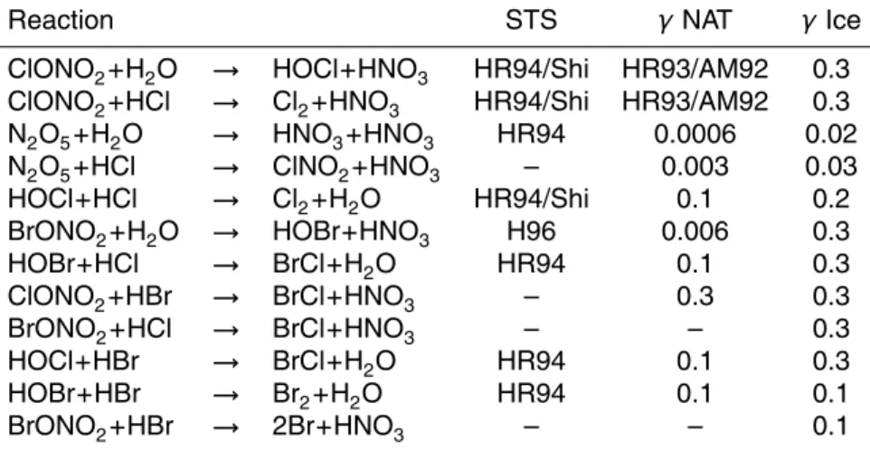
The heterogeneous chemistry module includes 30 different reactions on binary and ternary solutions, nitric acid trihydrate clouds and ice clouds (see Table 2). 14 reactions are added compared to Wohltmann et al. (2010).

The existence and composition of ternary solutions is calculated according to

20

Carslaw et al. (1995). Ternary solutions are formed only if no ice clouds exist. NAT or ice particles form if the saturation mixing ratios of HNO₃ over NAT or H₂O over ice exceed a given supersaturation. Saturation mixing ratios are calculated from the ex-pressions in Hanson and Mauersberger (1988) for NAT and Marti and Mauersberger (1993) for ice. NAT particles are assumed to form from the ternary solution droplets

25

(7)

ACPD

12, 26245–26295, 2012

depletion

I. Wohltmann et al.

Title Page

Tables Figures

◭ ◮

Back Close

Full Screen / Esc

Discussion

P

a

per

|

Dis

cussion

P

a

per

|

Discussion

P

a

per

|

Discussio

n

P

a

per

|

All particle types form instantly in equilibrium and are assumed to have a constant predefined number density. A uniform particle radius and a surface area density are calculated from the number density and the amount of HNO₃ or H₂O exceeding the saturation mixing ratio for NAT or ice clouds, respectively. In a similar way, the mean radius of a size distribution is adjusted for ternary solutions. The fractions of HNO₃,

5

H₂O and HCl contained in the cloud particles are not available for gas phase reactions. Technically, NAT clouds are formed before STS in the model, i.e. above the given supersaturation of HNO₃ over NAT, only NAT clouds and no ternary liquid clouds will exist, since they consume the available HNO₃. This is probably an overestimation of NAT occurence, since often, ternary liquids and NAT clouds are observed at the same

10

time (Pitts et al., 2011; Peter and Grooß, 2012).

The initialization of liquid H₂SO₄for the background aerosol has changed compared to Wohltmann et al. (2010). H₂SO₄mixing ratios have been reduced to a maximum of 0.12 ppb to make the surface area densities of the model compare better to surface area densities inferred from SAGE II. For this purpose, we fitted the calculated vortex

15

mean surface area densities of the reference run to the CCMVal surface area density climatology (Thomason and Peter, 2006) averaged over January to March of all years between 1997 to 2004 and latitudes north of 70◦_N.

Constant values for the gas-surface reaction probabilitiesγ on NAT and ice clouds

are employed in the model, with the exception of the reactions ClONO₂+HCl and

20

ClONO₂₊H₂O on NAT (Table 2). By default, we use the parameterization scheme 1 in Carslaw et al. (1997), which is based on the laboratory studies of Hanson and Rav-ishankara (1993). Alternatively, the scheme 2 of Carslaw et al. (1997), which is based on the studies of Abbatt and Molina (1992), can be used. By default, the reactions ClONO₂+HCl and ClONO₂+H₂O on ternary solutions are parameterized according

25

(8)

ACPD

12, 26245–26295, 2012

depletion

I. Wohltmann et al.

Title Page

Tables Figures

◭ ◮

Back Close

Full Screen / Esc

Discussion

P

a

per

|

Dis

cussion

P

a

per

|

Discussion

P

a

per

|

Discussio

n

P

a

per

|

aerosols only and is extended for ternary solutions as described in Wegner et al. (2012).

The denitrification module simulates the nucleation, transport, growth and sedimen-tation of a large number of PSC particles and is based on the DLAPSE model of Carslaw et al. (2002), for details see Wohltmann et al. (2010).

5

The model simulates two di_fferent modes of NAT particles: A small mode with parti-cles of about 1 µm radius on which the heterogeneous reactions take place, but which do not sediment in the model, and a large mode with radii of about 10 µm (“NAT rocks”, Fahey et al., 2001) in the particle module, which does not take part in the chemistry in the model. Here, we assume that the surface area density of the NAT rocks is small

10

enough to be negligible compared to the surface area of the small mode.

2.3 Model setup

Model runs are driven by meteorological data from the ECMWF ERA Interim reanalysis (Dee et al., 2011) on 60 model levels (6 h temporal resolution, 2◦

×2◦ horizontal

reso-lution). Horizontal model resolution is approximately 150 km (see Wohltmann and Rex,

15

2009) and vertical resolution is 1–2 km. The runs use the hybrid pressure-potential temperature coordinate of the model, which is a pure potential temperature coordi-nate above 100 hPa. The vertical motion is driven by diabatic heating rates (clear sky) from ERA Interim. The lower model boundary is at 350 K potential temperature and the upper boundary at 1900 K. Mixing strength by the critical Lyapunov exponent is set

20

to 3 d−1 _{(optimal mixing, see Wohltmann and Rex, 2009) and the mixing time step to}

12 h. The runs are started on 1 November 2009 and end on 31 March 2010. Chemical species are initialized on 1 December to allow for a spin-up in the mixing. Chemical species at the lower and upper boundary are re-initialized every 12 h, as described in Wohltmann and Rex (2009).

25

(9)

ACPD

12, 26245–26295, 2012

depletion

I. Wohltmann et al.

Title Page

Tables Figures

◭ ◮

Back Close

Full Screen / Esc

Discussion

P

a

per

|

Dis

cussion

P

a

per

|

Discussion

P

a

per

|

Discussio

n

P

a

per

|

active ozone is then a measure for chemical ozone depletion. In an equivalent way, a passive NO_y tracer is set up by adding up all nitrogen-containing species (except for N₂O and N₂). The di_fference between this tracer and NO_y is then a measure for denitrification by sedimenting particles.

The number density of NAT particles in the reference run is set to 0.1 cm−3_{, since} 5

this is an upper limit for the majority of measurements (e.g. Northway et al., 2002; Voigt et al., 2005; Pitts et al., 2009, 2011). For a more detailed discussion, see Drdla and M ¨uller (2012) or Peter and Grooß (2012). The number density of ice particles is set to 0.01 cm−3_{and the number density of the ternary solution droplets to 10 cm}−3_.

A supersaturation of 10 is assumed to be necessary for the formation of the NAT

10

particles (corresponding to about 3 K supercooling). This value is estimated from at-mospheric observations (e.g. Dye et al., 1990, 1992; Pitts et al., 2007) and laboratory work (Wagner et al., 2005), for discussion see Drdla and M ¨uller (2012) or Peter and Grooß (2012).

The Lagrangian particle model is used to simulate the nucleation, sedimentation,

15

growth and evaporation of large NAT particles. Particles are formed with a nucleation rate of 7.8×10−6particles per h and cm3(Voigt et al., 2005; Grooß et al., 2005) and an

initial radius of 0.1 µm, wherever the temperature is below the NAT equilibrium temper-ature.

2.4 Sensitivity runs

20

In addition to the reference run (REF), several sensitivity runs are carried out (Table 3): We explore the hypotheses of Drdla and M ¨uller with several runs that allow activa-tion only on liquid aerosol, but not on NAT or ice clouds. A run ONLY-LIQ-TER is per-formed that allows activation only on liquid ternary aerosols, but with everything else unchanged in the heterogeneous chemistry module. That is, the default rates of Shi

25

(10)

ACPD

12, 26245–26295, 2012

depletion

I. Wohltmann et al.

Title Page

Tables Figures

◭ ◮

Back Close

Full Screen / Esc

Discussion

P

a

per

|

Dis

cussion

P

a

per

|

Discussion

P

a

per

|

Discussio

n

P

a

per

|

and ClONO₂+H₂O on liquid aerosol instead of the default rates from Shi et al. (2001). Finally, we perform a run ONLY-LIQ-BIN that allows activation only on binary aerosols (no uptake of HNO₃) and uses the rates of Shi et al. (2001). NAT clouds were switched

offin the ONLY-LIQ-TER, ONLY-LIQ-TER-HR and ONLY-LIQ-BIN runs as a surrogate

for using the very slow reaction rates based on Abbatt and Molina (1992) and

prescrib-5

ing a low NAT surface area density, as done in the “NAT, current” case of Drdla and M ¨uller (2012).

In addition, a run ABBATT with the NAT reaction rates based on Abbatt and Molina (1992) is performed, which uses the same PSC parameterization as the reference run. This results in the same HNO₃ uptake on NAT clouds as in the reference run,

10

but in no heterogeneous activation on NAT due to the low reaction rates. That is, it is expected that the ABBATT run shows similar activation to the ONLY-LIQ-BIN run due to the small HNO₃ uptake by liquid aerosols. In the “NAT, current” case of Drdla and M ¨uller (2012), low surface area densities are assumed in addition. These either require very low number densities for NAT (10−4_cm−3 _{or lower) or gas-phase HNO}

3and NAT

15

to be in non-equilibrium for higher NAT number densities. Since our equilibrium model always uses all available HNO₃above the NAT saturation mixing ratio to form NAT, the results for the ABBATT run are independent of the NAT number density if the chlorine activation on the NAT clouds is negligible. However, if we had assumed non-equilibrium and higher NAT number densities to obtain the low NAT surface area density, uptake of

20

the additional gas-phase HNO₃ by liquids would have produced results similar to the ONLY-LIQ-TER run.

A run with a global temperature o_ffset of −1 K is used to study the sensitivity to

temperature changes (MINUS-ONE-KELVIN). Reaction rates for liquid aerosols show a large sensitivity to temperature changes. A typical order of magnitude for differences

25

(11)

ACPD

12, 26245–26295, 2012

depletion

I. Wohltmann et al.

Title Page

Tables Figures

◭ ◮

Back Close

Full Screen / Esc

Discussion

P

a

per

|

Dis

cussion

P

a

per

|

Discussion

P

a

per

|

Discussio

n

P

a

per

|

A run with the denitrification by sedimentation of large NAT particles switched off

(NO-DENITRI), and a run with the nucleation rate of “NAT rocks” multiplied by 10 (MORE-DENITRI) explore the sensitivity of the results to the simulated extent of deni-trification.

Several runs examine the sensitivity of the results to microphysical parameters,

5

which are still not well known (Peter and Grooß, 2012): a run with no supersaturation required for the formation of NAT particles (NO-SUPERSAT), a run with a supersatu-ration of 30 (5 K supercooling, MORE-SUPERSAT), a run with the number density of NAT particles set to 1 cm−3_(REF

×10, MORE-NATPART), and a run with the number

density of NAT particles set to 0.01 cm−3_{(REF/10, LESS-NATPART).} 10

We also tested the importance of ice clouds for chlorine activation. The reference run uses a supersaturation of 4, which e_ffectively switches ice clouds o_ff. A run with no supersaturation (not shown) shows identical results, which suggests that ice clouds play no role for the activation in this winter, even though they were observed in amounts unusual for the Arctic (Pitts et al., 2011).

15

Several of the sensitivity runs deliberately use unrealistic conditions (e.g. the number density in the MORE-NATPART run or no denitrification in the NO-DENITRI run) to show that even unrealistic changes do not cause large deviations from the reference run.

Chemistry is only calculated north of 30◦_{N latitude for the sensitivity runs to save} 20

computing time. South of 30◦_{N, the mixing ratios are constantly re-initialized with the}

results of the reference run.

2.5 Chemical initialization

H₂O, N₂O, HCl, O₃, CO and HNO₃ are initialized from all measurements of the MLS instrument on the Aura satellite performed during 1 December 2009 (Waters et al.,

25

(12)

ACPD

12, 26245–26295, 2012

depletion

I. Wohltmann et al.

Title Page

Tables Figures

◭ ◮

Back Close

Full Screen / Esc

Discussion

P

a

per

|

Dis

cussion

P

a

per

|

Discussion

P

a

per

|

Discussio

n

P

a

per

|

determined by calculating short backward trajectories from the time and location of the satellite measurement to the model initialization time.

CH₄is initialized from a monthly mean HALOE climatology (mean of the years 1991– 2002) as a function of equivalent latitude and pressure (Grooß and Russell III, 2005). All values are multiplied by 1.066 to account for the trend in CH₄ (e.g. WMO, 2011).

5

NO_xis initialized from the monthly mean HALOE data set by putting all NO_xinto NO₂. ClONO₂is calculated as the difference between Cl_yand HCl. Cl_yis taken from a Cl_y -N₂O tracer-tracer correlation from ER-2 aircraft and Triple balloon data (Grooß et al., 2002). The reference run and all sensitivity runs show a systematic and persistent bias compared to measurements with this initialization. That is, less ozone depletion

10

than observed (about 10 DU in the column), less chlorine activation (up to 0.4 ppb less ClO in sunlit conditions) and more HCl (up to 0.5 ppb). A run with ClONO₂taken from measurements of the MIPAS instrument onboard the Envisat satellite on 1 December, with the profiles retrieved by the Oxford L2 processor MORSE (http://www.atm.ox.ac. uk/group/mipas/) gave similar results (not shown in the following). Hence, we increase

15

ClONO₂by 10 %:

ClONO₂=1.1(Cl_y−HCl) (1)

HCl is decreased by the same amount to conserve Cl_y:

HCl_new=HCl−0.1 ClONO2 (2)

This leads to a better agreement between measurements and the reference run and all

20

sensitivity runs. However, there is still a moderate underestimation of chlorine activation in all runs. It seems not unlikely that the bias is indeed caused by small differences in the partitioning between HCl and ClONO₂, since small changes in the partitioning have a rather large e_ffect on the results of the model runs and the changes that define the sensitivity runs do not reduce the systematic bias in HCl.

25

(13)

ACPD

12, 26245–26295, 2012

depletion

I. Wohltmann et al.

Title Page

Tables Figures

◭ ◮

Back Close

Full Screen / Esc

Discussion

P

a

per

|

Dis

cussion

P

a

per

|

Discussion

P

a

per

|

Discussio

n

P

a

per

|

the organic source gases. The obtained Br_yis scaled by a constant factor to give max-imum Br_y values of 19.9 ppt to agree with Di_fferential Optical Absorption Spectroscopy (DOAS) measurements of BrO (Dorf et al., 2008).

CFCs and Halons (which have no relevant effects on the time scales considered in this study) are initialized as in Wohltmann et al. (2010).

5

3 Model results and comparison to observations

3.1 Meteorological situation

In the context of the Arctic stratospheric winters of the last decades, the winter of 2009/2010 was one of the more dynamically disturbed and warm winters. However, the polar vortex experienced an exceptionally cold phase for a short period during January

10

2010, when the vortex was relatively isolated and stable for several weeks (see also D ¨ornbrack et al., 2012, for more details).

The polar vortex formed in the early days of December 2009 at the 475 K level, on which we will concentrate here. Already during the formation phase of the vortex, a wave 2 event starting on 6 December split the vortex into two parts by 10 December.

15

The two parts reunited about 10 days later, but mixed in some extra-vortex air. The first temperatures below the NAT equilibrium temperature were observed around 17 De-cember. For the next four weeks, the vortex remained relatively stable and isolated. Temperatures remained low and reached the ice frost point on a synoptic scale around 15 January.

20

Starting a few days later, the vortex was gradually displaced to Siberia by a devel-oping major warming. The last temperatures below the ice frost point were observed around 25 January. The development of the major warming culminated at the end of January and beginning of February. The warming event was accompanied by a pro-nounced rise of the temperatures to more than 200 K almost everywhere in the vortex

25

(14)

ACPD

12, 26245–26295, 2012

depletion

I. Wohltmann et al.

Title Page

Tables Figures

◭ ◮

Back Close

Full Screen / Esc

Discussion

P

a

per

|

Dis

cussion

P

a

per

|

Discussion

P

a

per

|

Discussio

n

P

a

per

|

parts (one small part located over Canada and a larger part over Siberia) remained surprisingly stable until 1 March, when they were united again. The reunited vortex then remained stable for some weeks and finally dissipated.

Observations by the CALIPSO satellite (Pitts et al., 2011) show only patchy STS/NAT mixtures with low NAT number densities up to the end of December. The first half of

5

January was characterized by widespread STS/NAT mixtures with higher NAT number densities. From 15 to 21 January, synoptic scale ice clouds were observed, which is rare in the Arctic. The last PSC period, which lasted to the end of January, was domi-nated by STS clouds.

3.2 Chlorine activation

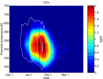
10

Figure 1 shows the vortex-averaged active chlorine (ClO_x=ClO+2 Cl₂O₂) of the refer-ence run as a function of time and potential temperature. Compared to colder winters, the period of chlorine activation was relatively short. Chlorine activation set in at the end of December and ClO_xreached maximum values of about 2.1 ppb in the second half of January, when the lowest temperatures were observed. Chlorine was deactivated very

15

quickly during early February, when the major warming set in.

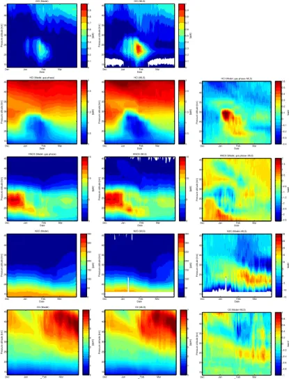
The comparison of the simulated ClO of the reference run with vortex means of satellite measurements of the MLS instrument (Fig. 2, top row) shows that the general morphology is matched well by the model. However, a quantitative comparison of the modeled and observed vortex average of ClO is difficult. The distribution of the local

20

times of the observations di_ffers from that of the model results, and these di_fferences in temporal sampling could give rise to di_fferences in their respective vortex average values.

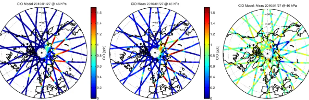
For a quantitative comparison, we calculated backward trajectories starting at se-lected satellite measurements and ending at the time of the last model output before

25

(15)

ACPD

12, 26245–26295, 2012

depletion

I. Wohltmann et al.

Title Page

Tables Figures

◭ ◮

Back Close

Full Screen / Esc

Discussion

P

a

per

|

Dis

cussion

P

a

per

|

Discussion

P

a

per

|

Discussio

n

P

a

per

|

(see Wohltmann et al., 2010, for details). Figure 3 shows the results for 27 January at 46 hPa, the results for additional dates can be found in Sect. 4 (Fig. S17) in the Sup-plement. The comparison indicates an underestimation of ClO by the model (typically 0.1–0.4 ppb). This is consistent with an overestimation of the vortex-averaged HCl of about 0.3 ppb by the model compared to MLS in the same time period and altitude

5

range (see next section). Hence, the underestimation is more likely caused by an un-derestimation of ClO_xthan by uncertainties in the partitioning between ClO and Cl₂O₂. The ClO measurements of MLS are corrected as described in Livesey et al. (2011) for the negative bias mentioned in Santee et al. (2008). The remaining uncertainties are around 0.1 ppb and cannot explain the differences between model results and

mea-10

surements.

However, ClO measurements of the HALOX instrument (von Hobe et al., 2005; Sumi ´nska-Ebersoldt et al., 2012) onboard the Geophysica agree well with the model results (see Sect. 1, Fig. S7, in the Supplement). But note that these measurements were obtained at about 430 K, where ClO mixing ratios are smaller. The reason for

15

the large discrepancy between the model and the profile measured on 30 January is unclear.

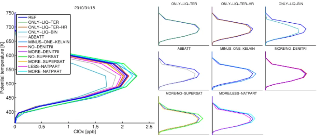
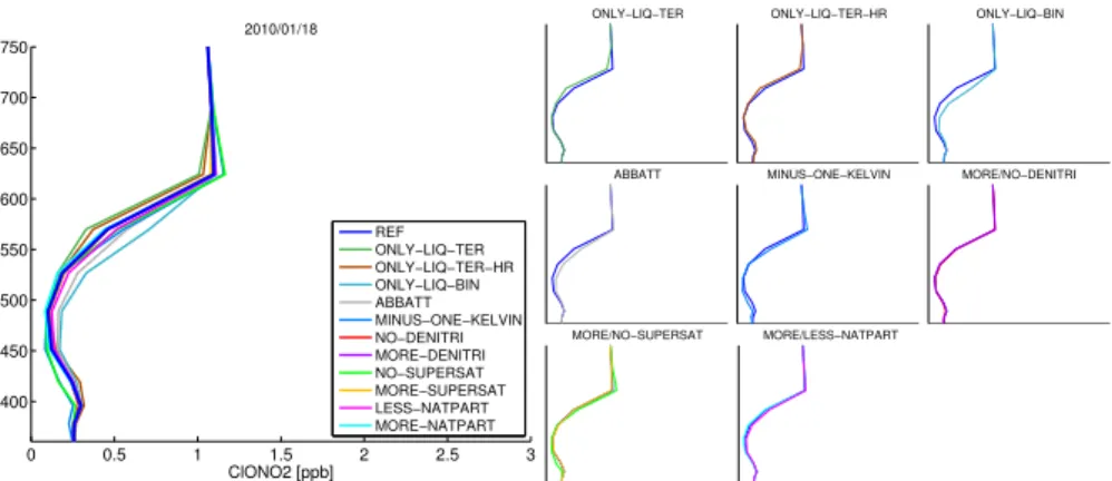
The left panel of Fig. 4 shows the vortex mean chlorine activation in all sensitivity runs and the reference run on 18 January 2010, when all runs show strong activation. The small plots on the right show the same data, but now only a single or two sensitivity

20

runs per plot for clarity. The runs show considerable di_fferences in the absolute amount of chlorine activation at the peak of the profile, ranging from 1.7 ppb for the ONLY-LIQ-BIN run to 2.3 ppb for the MINUS-ONE-KELVIN and NO-SUPERSAT runs. The reference run shows an activation of 2.1 ppb. The di_fferences between the peak mixing ratios in the sensitivity runs are within 30 %.

25

(16)

ACPD

12, 26245–26295, 2012

depletion

I. Wohltmann et al.

Title Page

Tables Figures

◭ ◮

Back Close

Full Screen / Esc

Discussion

P

a

per

|

Dis

cussion

P

a

per

|

Discussion

P

a

per

|

Discussio

n

P

a

per

|

chlorine activation and ozone depletion. The Shi et al. (2001) reaction rates in the ONLY-LIQ-TER run cause only a small increase of 0.1 ppb in the chlorine activation compared to the rates of Hanson and Ravishankara (1994) in the ONLY-LIQ-TER-HR run.

Chlorine activation in the reference run is almost identical to the ONLY-LIQ-TER

5

run and the MORE-SUPERSAT run (which shows 2.0 ppb). This suggests that the supersaturation in the reference run and the MORE-SUPERSAT run was so high that almost no NAT clouds formed. Notable di_fferences between the runs with and without NAT clouds can only be achieved by decreasing the supersaturation and increasing the NAT number densities.

10

The degree of chlorine activation is moderately larger in the runs with no super-saturation (NO-SUPERSAT) and more NAT particles (MORE-NATPART) due to the increased mean surface area density (2.3 ppb and 2.2 ppb, respectively). The opposite is true for the LESS-NATPART run (2.0 ppb). That is, even large changes in supersatu-ration and number density, which reach the limits of realistic values in the atmosphere,

15

do only cause changes in chlorine activation in the 10 % range.

The impact of changes in the denitrification on ClO_x is small on 18 January in the model. Larger di_fferences occur later in winter, when sunlight returns and the deac-tivation is hindered due to missing HNO₃ and NO_x. This can be seen clearly in the comparison of the ClO_xvalues of the NO-DENITRI run and the reference run in Sect. 6

20

(Fig. S30) in the Supplement. The NO-DENITRI shows lower ClO_x values since

de-activation into ClONO₂ is enhanced compared to the reference run. On 18 January, the NO-DENITRI run shows slightly higher ClO_x values since more NO_x is available to regenerate ClONO₂, which in turn is needed for the HCl₊ClONO₂ heterogeneous reaction.

25

(17)

ACPD

12, 26245–26295, 2012

depletion

I. Wohltmann et al.

Title Page

Tables Figures

◭ ◮

Back Close

Full Screen / Esc

Discussion

P

a

per

|

Dis

cussion

P

a

per

|

Discussion

P

a

per

|

Discussio

n

P

a

per

|

The ONLY-LIQ-BIN run shows the lowest activation of all sensitivity runs (1.7 pbb) due to the missing uptake of HNO₃ into the droplets and the decreased surface area density. But still, the results are of similar magnitude and are able to explain a large part of the observed chlorine activation and subsequent ozone depletion. The ABBATT run shows results similar to the ONLY-LIQ-BIN run (1.9 pbb). This is because HNO₃is

5

depleted from the gas-phase by the NAT clouds, but the reaction rates of Abbatt and Molina (1992) are very low.

It is di_fficult to decide between the runs with NAT and liquid aerosol and the runs with only liquid aerosol based on the comparisons between the model runs and the comparison of the model to measured species for this winter. However, our results show

10

that it is likely that liquid aerosols play an important role in the activation of chlorine, since NAT clouds are of second importance for the activation for current estimates of NAT number density and supersaturation.

Unfortunately, there are no usable measurements of Cl₂O₂for this winter so far, thus no comparison with measured ClO_xis possible.

15

3.3 Reservoir gases

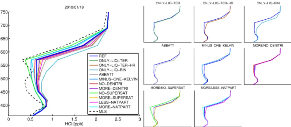
The evolution of the modeled HCl in the reference run compares well to the observa-tions of MLS morphologically (Fig. 2, 2nd row). However, HCl is overestimated in the model by about 0.3 ppb in the regions where HCl is depleted by reactions on PSCs.

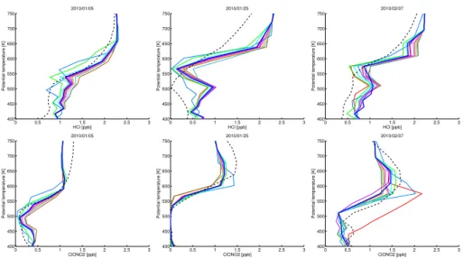
Figure 5 shows vortex mean HCl profiles on 18 January for all sensitivity runs. It is

20

obvious that the overestimation below 550 K is common to almost all sensitivity runs. A possible reason for the discrepancy could be that the reference initialization still un-derestimates the real ClONO₂ amount. That would hinder the activation of chlorine by the heterogeneous reaction ClONO₂₊HCl once that ClONO₂had been completely consumed. Further activation would only continue after reformation of ClONO₂by

pho-25

(18)

ACPD

12, 26245–26295, 2012

depletion

I. Wohltmann et al.

Title Page

Tables Figures

◭ ◮

Back Close

Full Screen / Esc

Discussion

P

a

per

|

Dis

cussion

P

a

per

|

Discussion

P

a

per

|

Discussio

n

P

a

per

|

There are other possible reasons for the discrepancies in HCl and ClO, e.g. a high temperature bias in the ERA Interim reanalysis. A global change of the temperature by -1 K in the MINUS-ONE-KELVIN run explains a large part of the discrepancy.

The good agreement between the NO-SUPERSAT run and the observations shows that it cannot be completely excluded that NAT clouds play a greater role in relation to

5

liquid clouds in reality than in our reference run, which shows almost no NAT PSCs. However, the vortex-wide formation of NAT clouds directly below the NAT equilibrium temperature is not supported by observations.

Figure 6 shows vortex mean ClONO₂ profiles, which all show very low values be-low about 525 K, indicating that most available ClONO₂ is used up in all sensitivity

10

runs. Above 600 K, ClONO₂ is not depleted. Figure S19 in Sect. 5 of the supplement shows that active chlorine is first transformed into ClONO₂starting in February, which is expected under Arctic conditions (e.g. M ¨uller et al., 1994).

Measurements of ClONO₂ for this winter were made by the ACE-FTS instrument

(Bernath et al., 2005). Since ACE-FTS is a solar occultation instrument, measurements

15

are more sparse than for the MLS instrument and are only available for the second half of the winter. In Fig. 7, we show some selected profiles of ClONO₂and HCl measured inside the vortex on di_fferent days in comparison with the model (version 3.0 data, more species can be found in Sect. 3, Figs. S14–S16, in the Supplement). The agreement of the simulated and observed ClONO₂is quite satisfactory below about 600 K. The ACE

20

measurements of HCl basically confirm the results of the comparison with MLS data. On 24 January, there was also a balloon ascent of the MIPAS-B instrument, which measured ClO, HCl and ClONO₂, but which we did not use here (Wetzel et al., 2012). Unfortunately, no instrument measures all of the important chlorine species at the same time (HCl, ClONO₂, ClO and Cl₂O₂), so that no definitive statements about the

agree-25

(19)

ACPD

12, 26245–26295, 2012

depletion

I. Wohltmann et al.

Title Page

Tables Figures

◭ ◮

Back Close

Full Screen / Esc

Discussion

P

a

per

|

Dis

cussion

P

a

per

|

Discussion

P

a

per

|

Discussio

n

P

a

per

|

3.4 Ozone loss

Figure 8 shows the vortex-averaged ozone loss as a function of time and potential temperature for the reference run. The largest loss rates are observed in the first half of February, shortly after the highest ClO_xvalues. After the warming, ozone loss continues until the end of the model run in March at a slower pace. Even though the vortex splits

5

into two parts and is subject to considerable mixing, ozone depleted air remains clearly visible until the end of March in the model. Maximum ozone loss values of 1.4 ppm are reached in the layer between 594 K and 655 K inside the vortex by the end of the winter (30 March).

Figure 9 shows the loss profiles for the reference run and all sensitivity runs on

10

30 March. The differences between the sensitivity runs are within 30 % (0.2 ppm). The potential temperature layer with the largest absolute differences between sensitivity runs is 471 K to 507 K. Ozone loss values are between 0.78 ppm and 0.95 ppm in this layer. Ozone loss is only slightly underestimated compared to MLS in this altitude range. Above about 600 K, NO_x-induced loss begins to dominate (note the decrease

15

in ClO_x in Fig. 1), but this region only plays a relatively small role for the column. Here, most runs agree well, since the e_ffects of heterogeneous chemistry begin to

decrease. The MINUS-ONE-KELVIN run shows lower ozone loss here, since the NO_x

cycle is more e_ffective at higher temperatures. The maximum ozone loss in the model is underestimated compared to the MLS loss of 1.6 ppm.

20

Figure 10 shows the corresponding loss in the ozone column for the reference run and all sensitivity runs. The column loss in the reference run on 30 March amounts to 77 DU over the complete simulated column and to 58 DU below 600 K (better compa-rable to results of methods that deduce ozone loss from sonde observations, like the vortex-average method, which typically yield no results above 600 K). The simulated

25

(20)

ACPD

12, 26245–26295, 2012

depletion

I. Wohltmann et al.

Title Page

Tables Figures

◭ ◮

Back Close

Full Screen / Esc

Discussion

P

a

per

|

Dis

cussion

P

a

per

|

Discussion

P

a

per

|

Discussio

n

P

a

per

|

at the end of the winter differs only by a maximum of 7 DU between the sensitivity runs (less than 10 %), showing that even large changes in the underlying assumptions on heterogeneous chemistry have only a relatively small impact on the modeled column ozone loss.

The di_fferences of the sensitivity runs are to some extent sensitive to the exact

pro-5

cedure of averaging. In particular, taking 1 March as the ending date for the columns would give larger differences (up to 15 %), since after 1 March, the differences between the sensitivity runs and the reference run in ozone depletion decrease (see the di_ff er-ence of ozone loss between the sensitivity runs and the referer-ence run in Sect. 6 in the Supplement, which peak around 1 March). The decrease is probably caused by

10

our vortex definition, which includes more and more mid-latitude air, since the vortex shrinks faster than we assume.

Likewise, calculating partial columns only up to 600 K also increases the percentage (up to 13 % on 30 March), since most of the di_fferences in the sensitivity runs occur below 600 K. Combining both e_ffects gives di_fferences of up to 20 %.

15

Comparison of vortex-averaged model ozone to MLS measurements shows a slight overestimation of ozone by the model (Fig. 2, 5th row), in line with the results for HCl and ClO of the last subsection. Accordingly, the column ozone loss of 82 DU obtained from MLS by subtracting the passive ozone tracer of the model from the MLS ozone measurements is slightly larger than the modeled loss in most sensitivity runs (see

20

Fig. 10). The NO-SUPERSAT run shows the best agreement, with a column loss of 81 DU at the end of March.

Measurements from ozone sondes and from the FOZAN instrument onboard the Geophysica (Ulanovsky et al., 2001) generally show a good agreement with the simu-lated ozone and also roughly confirm the simusimu-lated ozone loss (see Sect. 1, Fig. S8,

25

(21)

ACPD

12, 26245–26295, 2012

depletion

I. Wohltmann et al.

Title Page

Tables Figures

◭ ◮

Back Close

Full Screen / Esc

Discussion

P

a

per

|

Dis

cussion

P

a

per

|

Discussion

P

a

per

|

Discussio

n

P

a

per

|

3.5 Denitrification

Although the vortex was relatively disturbed (D ¨ornbrack et al., 2012), pronounced den-itrification was simulated by the model in the reference run (Fig. 11). Denden-itrification set in at the beginning of January in the model with the low temperatures and reached maximum values of 7.5 ppb in the second half of January. The air remained denitrified

5

until the end of the model run in March. Below the denitrified layer, a renitrified layer with values of up to 3.3 ppb is simulated.

Figure 12 shows NO_y (left panel) and HNO₃(right panel) for the reference run and the relevant sensitivity runs on 2 February 2010. 2 February is around the peak of denitrification, but on a day with no uptake of HNO₃ by PSCs in the model, which

10

would complicate the comparison. In addition, the CALIPSO satellite instrument shows no PSCs on this day (Pitts et al., 2011). Note that the passive NO_ytracer is identical to the modeled NO_yof the NO-DENITRI run (red line), i.e. the difference between the red line and any other line quantifies the denitrification. On this day, the reference run (and all other runs using the nucleation rate of the reference run except for the

MINUS-ONE-15

KELVIN run) shows a denitrification of 7.3 ppb and a renitrification of 3.0 ppb, while the MORE-DENITRI run (nucleation rate multiplied by 10) shows 8.8 ppb denitrification and 3.9 ppb renitrification. The MINUS-ONE-KELVIN run shows more denitrification than the reference run since the lower temperatures lead to larger areas below the NAT equilibrium temperature and a faster particle growth.

20

Comparison with vortex-averaged observations of HNO₃by MLS (e.g. for 2 February in the right panel) shows that the runs with the standard nucleation rate of the reference run usually show the best agreement with the measurements. The run with no denitrifi-cation is clearly not compatible with the measurements. The MORE-DENITRI run and the MINUS-ONE-KELVIN run often show lower values than the measurements.

25

(22)

ACPD

12, 26245–26295, 2012

depletion

I. Wohltmann et al.

Title Page

Tables Figures

◭ ◮

Back Close

Full Screen / Esc

Discussion

P

a

per

|

Dis

cussion

P

a

per

|

Discussion

P

a

per

|

Discussio

n

P

a

per

|

underestimated by the model (by less than 2 ppb), hinting at a small overestimation of the denitrification by sedimenting particles in the model in the reference run.

3.6 Long-lived tracers

A proper simulation of transport and mixing is a prerequisite for a model simulation of high quality. In addition, it excludes transport as a source of differences between

5

model and measurement and allows attribution of the di_fferences to e.g. the initializa-tion or chemistry scheme. A large number of long-lived tracers was measured on the Geophysica flights by the HAGAR instrument (Volk et al., 2000). We will concentrate on N₂O and CH₄measurements since all tracers basically allow the same conclusions and N₂O was additionally measured by MLS.

10

The flights generally show excellent agreement between model results and mea-surements, indicating no major problems (see Sect. 1, Figs. S9 and S10, in the Sup-plement). This is supported by the good agreement between model and MLS

mea-surements up to February. Figure 2 shows an overestimation of N₂O by the model

compared to MLS of up to 20 ppb between 20 to 25 km in February and March. There

15

are two possible reasons for this: either an underestimation of diabatic descent in the vortex or an overestimation of the in-mixing of air rich in N₂O from outside the vortex.

Di_fferences in heating rates and mixing between model and reality can cause dis-crepancies between measurements and model. E.g., an overestimation of mixing across the vortex edge would cause lower chlorine values and less ozone loss. It is

20

di_fficult to quantify how large these e_ffects are, since that would require knowledge about the correct mixing and heating rates.

4 Discussion

CALIPSO satellite measurements indicate that both STS and NAT clouds were ubiqui-tous in the Arctic vortex in the winter 2009/2010 (Pitts et al., 2011), with number

(23)

ACPD

12, 26245–26295, 2012

depletion

I. Wohltmann et al.

Title Page

Tables Figures

◭ ◮

Back Close

Full Screen / Esc

Discussion

P

a

per

|

Dis

cussion

P

a

per

|

Discussion

P

a

per

|

Discussio

n

P

a

per

|

sities in a broad range from 0.001 cm−3_{to 0.1 cm}−3_{and even higher. In comparison to}

the other three Arctic winters observed by CALIPSO since 2006/2007, an enhanced number of high density (>0.1 cm−3_{) STS/NAT mixture clouds was observed. A}

pecu-liarity of this winter was the widespread existence of synoptic-scale ice clouds, which were rarely observed in other Arctic winters by CALIPSO.

5

CALIPSO observed NAT clouds in significant quantities in this winter. Nevertheless, the runs with activation only or mainly on liquid aerosols (TER, ONLY-LIQ-TER-HR, ONLY-LIQ-BIN, ABBATT, MORE-SUPERSAT) show that assuming activation on liquid aerosols only is able to explain the observed magnitude and morphology of the mixing ratios of active chlorine, reservoir gases and ozone. STS clouds were observed

10

virtually during the complete period where PSC formation was possible. In addition, the onset of chlorine activation in late December was dominated by clouds with a very low NAT number density (Pitts et al., 2011). A definitive assessment of how important activation on NAT is compared to activation on liquid aerosols is not possible with our results, since the results for the runs with and without NAT clouds are very similar.

15

Notable di_fferences can only be achieved by increasing the NAT number density and decreasing supersaturation. But even then, the results for the runs with and without NAT clouds are of the similar magnitude.

Based on the information from the laboratory studies alone, it is not possible to de-cide a priori whether the reaction rates of Abbatt and Molina (1992) or Hanson and

20

Ravishankara (1993) on NAT clouds are closer to reality (Carslaw et al., 1997). In ad-dition, due to the small amount of NAT clouds that form in the reference run and the ABBATT run, both runs give relatively similar results. A set of model runs that were performed in preparation of this study and which use a NAT number density of 1 cm−3

and a supersaturation of 4 shows that chlorine activation would be relatively small with

25

(24)

ACPD

12, 26245–26295, 2012

depletion

I. Wohltmann et al.

Title Page

Tables Figures

◭ ◮

Back Close

Full Screen / Esc

Discussion

P

a

per

|

Dis

cussion

P

a

per

|

Discussion

P

a

per

|

Discussio

n

P

a

per

|

significant quantities in this winter, but if our model runs favor the rates of Hanson and Ravishankara (1993) over those of Abbatt and Molina (1992) depends on their surface area relative to the liquid clouds, which is not well known.

Further, it is not easy to distinguish between the rates of Shi et al. (2001) or Hanson and Ravishankara (1994) for liquid aerosols in the model. At least in our model runs for

5

the winter 2009/2010, the change between the rates does not have a great impact on the results.

Our model assumes that NAT clouds are formed from STS droplets. There are con-siderable theoretical problems with this approach and the formation pathways for NAT are uncertain (Lowe and MacKenzie, 2008; Peter and Grooß, 2012). A possible

alter-10

native would be the nucleation of NAT on ice (Lowe and MacKenzie, 2008; Peter and Grooß, 2012). But on the other hand, NAT PSCs have clearly been observed without the prior formation of ice clouds (Voigt et al., 2005; Pitts et al., 2011). In particular, this is also the case for the winter 2009/2010 (Pitts et al., 2011). An inclusion of the ice mechanism into the model would produce less NAT clouds than the current mechanism

15

if only synoptic scale clouds are considered, but could be modified by assuming tem-perature fluctuations by mountain waves. Another alternative would be heterogenous nucleation on e.g. meteoric material (Lowe and MacKenzie, 2008; Peter and Grooß, 2012). That could be modelled by using the current algorithm, but by switching offthe correction for STS number density. This would give very similar results to the original

20

mechanism in the model.

The weak dependence of the results on the number density of NAT particles is not too surprising. If a given constant amount of HNO₃is distributed on a variable number

N of particles, a simple calculation shows that the corresponding surface area is pro-portional toN1/3. That is, increasing the number density by a factor of 10 increases the

25

surface area only by a factor of 101/3≈2.

(25)

chem-ACPD

12, 26245–26295, 2012

depletion

I. Wohltmann et al.

Title Page

Tables Figures

◭ ◮

Back Close

Full Screen / Esc

Discussion

P

a

per

|

Dis

cussion

P

a

per

|

Discussion

P

a

per

|

Discussio

n

P

a

per

|

istry and microphysics module and insufficient constraints by theory and observations. E.g., the model assumes an immediate equilibrium, while in reality, the formation and evaporation of cloud particles is a complex non-equilibrium process. This is true in par-ticular for NAT particles, e.g. the time required to condense 50 % of available HNO₃ in the gas-phase to NAT particles at a concentration of 10−3_cm−3_{is several days (Fig. 3 in} 5

Drdla and M ¨uller, 2012). In addition, a spatially and temporally constant number density is assumed for NAT, STS and ice, and all particles are assumed to have the same size. In reality, complex mixtures of di_fferent particle types, di_fferent number densities and different size distributions exist depending on the environmental conditions, air mass history and species concentrations. However, measurements are scarce and the exact

10

formation pathways of cloud particles are still not clear (Lowe and MacKenzie, 2008; Peter and Grooß, 2012). That makes it di_fficult to constrain the module su_fficiently by observations and theory. In addition, the module has to work fast and reliably under all environmental conditions that the model produces.

Our study is somewhat hampered by the fact that there is a persistent bias in all

15

sensitivity runs. All runs show less active chlorine, more reservoir gases and less ozone loss than the observations. However, we believe that the relative changes between the runs still provide valuable information that is not a_ffected by the bias. There are several possible factors that could easily explain the bias (a high temperature bias in the analysis, a systematic error in the ClONO₂ initialization, or a bias in the heating

20

rates or mixing across the vortex edge in the analysis). However, which explanation or combination of explanations is correct is not possible to determine with the available information.

Fortunately, there is a simple reason why all these uncertainties are of secondary importance in the end: Even large changes in the underlying assumptions have only

25

(26)

ACPD

12, 26245–26295, 2012

depletion

I. Wohltmann et al.

Title Page

Tables Figures

◭ ◮

Back Close

Full Screen / Esc

Discussion

P

a

per

|

Dis

cussion

P

a

per

|

Discussion

P

a

per

|

Discussio

n

P

a

per

|

but somewhat larger (up to 30 % on 18 January). Since it can be expected that ozone loss is roughly linear in ClO_x(Harris et al., 2010), the di_fferences in ozone loss are well explained by the differences in ClO_x.

There may be several reasons why the sensitivity of ozone loss to the changes seems to be even smaller than the sensitivity of ClO_x to the changes: First, our

vor-5

tex definition reduces the differences in ozone depletion between the sensitivity runs in late March, since more and more mid-latitude air is included in the average. Another reason is that the exact timing and altitude dependence of the activation are not impor-tant as long as the extent of the chlorine activation is the same in the end. Harris et al. (2010) demonstrate that several processes offset each other, e.g. the altitude

depen-10

dence of the reaction rates is o_ffset by the altitude dependence of Cl_y and the initially higher ozone loss rates in case of late activation are offset by faster deactivation. Fig-ure 13 illustrates this very convincingly. The figFig-ure shows the mean ClO_x of the winter versus the column ozone loss on 1 March for all sensitivity runs. There is an almost perfect linear relationship between the mean chlorine activation and the column ozone

15

loss.

5 Conclusions

We performed sensitivity runs for the Arctic winter 2009/2010 with the Lagrangian Chemistry and Transport Model ATLAS to explore the impact of uncertainties in chlo-rine activation and denitrification on the model results, with a particular focus on

micro-20

physics and chemistry on polar stratospheric clouds. Our main findings are:

– Even (unrealistically) large changes in the underlying assumptions have only a small impact on the modeled ozone loss. Changes in column ozone loss stayed below 10 % in our sensitivity runs. This shows that ozone loss is a robust quantity with regard to changes in the microphysical and chemical assumptions.

(27)

ACPD

12, 26245–26295, 2012

depletion

I. Wohltmann et al.

Title Page

Tables Figures

◭ ◮

Back Close

Full Screen / Esc

Discussion

P

a

per

|

Dis

cussion

P

a

per

|

Discussion

P

a

per

|

Discussio

n

P

a

per

|

– Chlorine activation on liquid aerosols alone is sufficient to explain the observed magnitude and morphology of the mixing ratios of active chlorine, reservoir gases and ozone.

– This is even true for binary aerosols (no uptake of HNO₃ from the gas-phase allowed in the model). However, the runs with ternary aerosols agree better with

5

the observations.

– No decision between the reaction rates of Shi et al. (2001) or Hanson and Rav-ishankara (1994) for liquid aerosols is possible from our results. The change be-tween the rates only has a minor impact on the results.

– The same is true for the rates of Abbatt and Molina (1992) or Hanson and

Rav-10

ishankara (1993) on NAT. However, one of the sensitivity runs with the rates of Abbatt and Molina (1992) indicates that chlorine activation would be relatively small with these rates, if at the same time NAT clouds in appreciable amounts existed. This is however not the case with our default values for supersaturation and number density.

15

– The timing and altitude dependence of the chlorine activation are not important in the model as long as the extent of the chlorine activation (ClO_x mixing ratio averaged over winter and all altitudes) is the same.

Our results are confirmed by the findings of Drdla and M ¨uller (2012) and Wegner et al. (2012). Wegner et al. (2012) show that there is no interannual correlation between the

20

depletion of HCl and the formation of NAT or STS clouds and that binary aerosol is su_fficient to explain the observed chlorine activation for several trajectory case studies in 2005 and 2010.

Supplementary material related to this article is available online at: http://www.atmos-chem-phys-discuss.net/12/26245/2012/

25

(28)

ACPD

12, 26245–26295, 2012

depletion

I. Wohltmann et al.

Title Page

Tables Figures

◭ ◮

Back Close

Full Screen / Esc

Discussion

P

a

per

|

Dis

cussion

P

a

per

|

Discussion

P

a

per

|

Discussio

n

P

a

per

|

Acknowledgements. We thank ECMWF for providing reanalysis data, Nathaniel Livesey and

the MLS science team at JPL for their support, the ACE team for providing ACE-FTS data, and Anu Dudhia and the University of Oxford for the MIPAS data. Work at the Jet Propulsion Laboratory, California Institute of Technology, was done under contract with the National Aero-nautics and Space Administration. The Atmospheric Chemistry Experiment (ACE) mission is

5

funded mainly by the Canadian Space Agency. Work at AWI, FZ J ¨ulich and University of Wup-pertal was supported by the EC DG research through the RECONCILE project (RECONCILE-226365-FP7-ENV-2008-1) and work at AWI was additionally supported by the SHIVA project (SHIVA-226224-FP7-ENV-2008-1).

References

10

Abbatt, J. P. D. and Molina, M. J.: Heterogeneous interactions of ClONO2and HCl on nitric acid

trihydrate at 202 K, J. Phys. Chem., 96, 7674–7679, 1992. 26248, 26251, 26254, 26261, 26267, 26268, 26271, 26280, 26281

Bernath, P. F., McElroy, C. T., Abrams, M. C., Boone, C. D., Butler, M., Camy-Peyret, C., Carleer, M., Clerbaux, C., Coheur, P.-F., Colin, R., DeCola, P., DeMazi `ere, M., Drummond, J. R.,

15

Dufour, D., Evans, W. F. J., Fast, H., Fussen, D., Gilbert, K., Jennings, D. E., Llewellyn, E. J., Lowe, R. P., Mahieu, E., McConnell, J. C., McHugh, M., McLeod, S. D., Michaud, R., Midwinter, C., Nassar, R., Nichitiu, F., Nowlan, C., Rinsland, C. P., Rochon, Y. J., Rowlands, N., Semeniuk, K., Simon, P., Skelton, R., Sloan, J. J., Soucy, M.-A., Strong, K., Tremblay, P., Turnbull, D., Walker, K. A., Walkty, I., Wardle, D. A., Wehrle, V., Zander, R., and Zou,

20

J.: Atmospheric Chemistry Experiment (ACE): Mission overview, Geophys. Res. Lett., 32, L15S01, doi:10.1029/2005GL022386, 2005. 26249, 26262

Burkholder, J. B., Orlando, J. J., and Howard, C. J.: Ultraviolet absorption cross sections of

chlorine oxide (Cl2O2) between 210 and 410 nm, J. Phys. Chem., 94, 687–695, 1990. 26250

Carslaw, K., Peter, T., and M ¨uller, R.: Uncertainties in reactive uptake coefficients for solid

25

stratospheric particles – 2. Effect on ozone depletion, Geophys. Res. Lett., 24, 1747–1750,

1997. 26248, 26251, 26267

Carslaw, K. S., Luo, B., and Peter, T.: An analytical expression for the composition of aqueous

HNO3-H2SO4stratospheric aerosols including gas phase removal of HNO3, Geophys. Res.

Lett., 22, 1877–1880, 1995. 26250