Development of bioinformatics tools to track cancer cell invasion using 3D in vitro invasion assays

(1)

F

ACULDADE DE

E

NGENHARIA DA

U

NIVERSIDADE DO

P

ORTO

Development of bioinformatics tools to

track cancer cells invasion using 3D in

vitro invasion assays

Rui Sérgio Malheiro Caldeira

Report of Project/Dissertation

Integrated Master in Electrical and Computer Engineering Supervisor: Pedro Quelhas (PhD)

(2)

c

(3)

Development of bioinformatics tools to track cancer cells

invasion using 3D in vitro invasion assays

Rui Sérgio Malheiro Caldeira

Report of Project/Dissertation

Integrated Master in Electrical and Computer Engineering

Approved in oral examination by the committee:

Chair: Name of the President (Title)

External Examiner: Name of the Examiner (Title)

Internal Examiner: Name of the Examiner (Title)

(4)

(5)

Resumo

Nas últimas décadas, o desenvolvimento de métodos de processamento de imagem utiliza-dos para investigação na área da Biologia, têm sido alvo de vários estuutiliza-dos. Considerando que as doenças da actualidade, tais como o cancro, encontram a sua cura dependente do estudo do comportamento celular, tornou-se necessário desenvolver ensaios de invasão ca-pazes de simular as características do tecido celular nas quais as células se desenvolvem. Uma vez que muitos dos projectos de investigação recorrem ao uso de microscópios, a necessidade de boas condições de visualização torna-se imperativa para a evolução dos estudos. Assim sendo, os ensaios de invasão são observados com profundidades difer-entes, permitindo uma melhor análise da extensão vertical alcançada pelas células - estas são depositadas no cimo do ensaios. A visualização dos espécimes através do microscó-pio sofre de um problema de ordem física caracterizado pelas aberrações causadas pela exposição à luz que indirectamente causa desfoque e névoa capturada pela lente do mi-croscópio. A influência destas limitações em imagens de microbiologia é inconveniente para qualquer investigação já que pode ocultar detalhes relevantes. Como forma de mini-mizar estas limitações, recorre-se a algoritmos de processamento de imagem tais como a desconvolução, para realce do objecto de estudo. A desconvolução restaura a exposição do objecto à luz e à névoa que provocam desfoque, bem como promove melhoramentos no contraste da imagem.

Neste artigo foram estudadas e desenvolvidas ferramentas de análise de imagem ca-pazes de identificar e quantificar células em ensaios de invasão. Foram também apresenta-dos e analisaapresenta-dos os resultaapresenta-dos apresenta-dos métoapresenta-dos de desconvolução aplicaapresenta-dos (“no neighbors”, “nearest neighbors”, desconvolução linear 2D / 3D e desconvolução “blind”), os resul-tados do algoritmo detector de células (composto por métodos de simetria de fase para detecção de cristas nas imagens e pela transformada de Hough para detecção de células com base na intensidade dos pixels que as compõem) e os resultados da comparação entre os métodos de estimação de focagem Laplaciano e baseados em intensidade (Hough) para estimação de profundidade das células.

(6)

(7)

Abstract

The development of image processing methods for Biology research has been the subject of several projects for the last decades. Considering that nowadays diseases, like cancer, have their possible cures depending on the study of cells behavior, it became necessary to develop invasion assays capable of emulating the tissue conditions in which cells evolve. As most of the research relies on the use of microscopy techniques, the need for good imaging conditions becomes imperative for the evolution of the studies. The assay is im-aged at different depths permitting a better visualization of the vertical extent reached by cancer cells - as they’re deposited on the top of the assay. The visualization of specimens using microscopes suffer from physical obstacles due to the aberrations caused by the ex-posure to out-of-focus light and haze, captured by the microscope lens. The presence of these obstacles in microbiology images is a serious drawback for any research as it may occlude important details. One way of subduing these obstacles is to process the images with algorithms capable of enhancing them like deconvolution methods. Deconvolution aims at restoring the out-of-focus light back to it’s source point, reducing the blur and providing better contrast.

In this article we study and develop image analysis tools to track and quantify the cells in an invasion assay. We’ll present and analyze the results of the deconvolution methods used (no neighbors, nearest neighbors, linear 2D / 3D deconvolution and blind deconvolution), the results of our cell detection algorithms (composed of phase symmetry for ridge detection and Hough transform for detecting cells based on intensities of the pixels) and the results of the comparison between a focus estimation method (Laplacian) and a Hough intensity based method for depth estimation purposes.

(8)

(9)

Acknowledgments

To my parents and my sister for all the care, support and dedication all through these years.

To my Dissertation supervisor, Pedro Quelhas, for his availability and readiness. To everybody who helped me at the INEB (Instituto de Engenharia Biomédica - Biomed-ical Engineering Institute, Porto), specially Lúcio Alves, Christophe Silva and Mónica Marcuzzo.

To all my close friends Bruno Brito, Bruno Ferreira, Bruno Ribeiro, Inês Novo, João Guerreiro, Nuno Covas, Pedro Pires and, at last but not the least, Renan Ramos.

To all of them, my sincere gratitude.

Rui Caldeira

(10)

(11)

“Morality, like art, means drawing a line someplace.”

Oscar Wilde

(12)

(13)

List of Figures

1.1 3D image acquisition of a cell [1]. . . 2

2.1 Schematic of (a) confocal and (b) brightfield microscopes [1]. . . 5

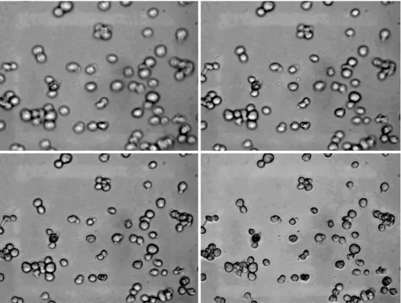
2.2 Example of an image stack: assay at different focus (from left to right, top to bottom). . . 9

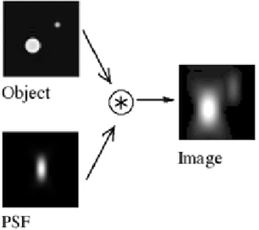
3.1 Image formation in a microscope: central longitudinal (X Z) slice. The 3D acquired distribution arises from the convolution of the real light sources with the PSF. . . 13

3.2 The 2D Gaussian distribution. . . 15

3.3 No neighbors results: original vs. processed. . . 15

3.4 Nearest neighbors results: original image versus processed. . . 17

3.5 2D Linear deconvolution results: original image versus processed. . . 19

3.6 3D Linear deconvolution results: original image versus processed. . . 19

3.7 Blind deconvolution results: original image versus processed. . . 21

3.8 Phase symmetry detection: original, phase symmetry (from left to right). . 23

3.9 Each point in the image space (left) generates a circle in the accumulator space (right). The circles in the accumulator space intersect at the (x, y) coordinates which is the center of the circle in the image space. . . 23

3.10 Hough transform: original, phase symmetry, Hough transform accumu-lator space and the representation of the maximum Hough detected point (from left to right, top to bottom). . . 24

3.11 Cell detection: original image on the left and detected cell image on the right. . . 25

3.12 Depth estimation using the Laplacian operator. . . 27

3.13 Depth estimation using the Hough transform estimator. . . 28

4.1 No neighbors results: original vs. deblurred. . . 30

4.2 Nearest neighbors results: original vs. deblurred. . . 32

4.3 Linear 2D deconvolution results: original vs. deconvolved. . . 33

4.5 Blind deconvolution results: original vs. deconvolved. . . 35

4.6 No neighbors results: original vs. deblurred. . . 37

4.7 Nearest neighbors results: original vs. deblurred. . . 37

4.10 Blind deconvolution results: original vs. deconvolved. . . 39

4.11 Depth estimation input stack of images. . . 39

(16)

xii LIST OF FIGURES

4.12 Depth estimation results: Laplace focus estimation. . . 40

4.13 Depth estimation results: Hough response based estimation. . . 41

4.14 Depth estimation results: Laplacian estimation vs. Hough response based estimation. . . 42

(17)

Abbreviations and Symbols

PSF Abbreviation for the point-spread function, which is the 3D image of a point source

Algorithm Computerized procedure to carry out a calculation

Deconvolution Method to undo the degradations introduced by an imaging process; a microscopic image is described mathematically as the convolution of the PSF with the object; to retrieve the original object from the image data, deconvolution is required

Pixel Abbreviation for picture element; the image is composed of a grid of picture elements, each with an intensity corresponding to the local in-tensity at that point in the specimen

Voxel 3D pixel, a volume element, incorporating the step size between focal planes as the third dimension; the 3D image is built from a 3D grid of voxels

X, Y , Z Coordinates for a 3D image; XY correspond to the focal-plane (or lateral) coordinates and Z corresponds to the direction of focal-plane change (or axial) coordinates

Optical axis Z axis

(18)

(19)

Chapter 1

Introduction

Since the 19th century, with the use of microscopes in Science and the discovery of cells, Biology gained a whole new meaning and suffered a huge revolution in its procedures. The knowledge of cells as the basic unit of which all living things are composed revolu-tionized the scientific community, bringing in a new chapter to the Scientific Revolution.

Nowadays Microbiology gathers efforts for the development and research of solutions to illnesses like cancer. Deaths from cancer worldwide are projected to continue rising, with an estimated 12 million deaths in 2030 [2]. As cancer being the leading cause of death worldwide, knowing how cancer evolves it’s imperative.

Cancer arises from a change in one single cell and the change may be started by external agents and inherited genetic factors. The compromising behavior of one cell affects all the others around it, spreading the abnormality throughout the tissues. During invasion, cancer cells establish a continuous molecular crosstalk with host elements of the surrounding microenvironment similar to the effect for which has been named - cancer; latin for crab. The necessity to examine the progression of cancer cells in the tissues and to study the interactions established between invasive cells and the other elements of the tumor microenvironment, led to the development of invasion assays capable of emulating the conditions in which cancer cells spread out.

An invasion assay consists of gels of extracellular matrix components (collagen type I or Matrigel, for instance), intermixed or not with macrophages or fibroblasts on top of which isolated cancer cells are added [3] and is used to analyze the expansion of the isolated top layer (cancer) cells downwards and quantify the number of cells involved in the progression.

Therefore the research on cancer cells is performed through observations of microscopy images (in digital format), taken from the assay at different depths. Those sequence of

(20)

2 Introduction

microscopy images are usually referred as stacks. Stacks of images enable us to deter-mine the relative position of a specimen in the assay and can be used to perform the 3D reconstruction of each specimen as they are equivalent to a series of microtome slices -see Figure1.1.

Figure 1.1: 3D image acquisition of a cell [1].

Considering the several different types of microscopes used for biology studies, in the next chapter (Chapter2), we’ll present and state a comparison between two often used mi-croscopes in Biology: confocal and brightfield. As an important note, the stack presented in this work is obtained from brightfield microscopy, through focal length variation.

The aim of this work is to study and develop image analysis tools for microscopy, to track and quantify cell invasion in an assay. In order to detect the depth of the cells on the images of the stack, we must create a detection algorithm capable of relating each cell to a specific image of the stack - given that each image represents a certain depth. But, imaging an assay with a brightfield doesn’t provide sufficient information to correctly relate cells to certain depths. For that reason, we’ll use deconvolution or focus estimation methods.

Deconvolution aims at removing out-of-focus haze from objects in images. As the im-ages are associated to different depth measures, preprocessing with deconvolution should improve in-focus, reducing contributions of out-of-focus cells information.

(21)

Introduction 3

image. Depth of each cell can be estimated by comparing the amount of focus, for the same (x, y) region, at different z planes. The true z location of the cell will be the point of highest focus estimation.

The main software developing platform used in the development project is Matlab R2007bR

though some use of ImageJ libraries are considered even if just for comparison procedures of the results.

The reminder of this work is organized as follows: in Chapter 2 we’ll talk about two frequently used types of microscopes applied for this kind of research; in Chapter3

we’ll unveil and describe the algorithms used: preprocessing methods as deconvolution and focus estimation and the detection algorithm; in Chapter4we’ll discuss the results; finally, Chapter5reveals the conclusions about the presented work.

(22)

(23)

Chapter 2

Microscopy

Optical microscopy involves diffraction, reflection or refraction of electromagnetic radi-ation / electron beam interacting with the subject of study, and the subsequent collection of this scattered radiation in order to build up an image. This process may be carried out by wide-field irradiation of the sample (for example standard light microscopy as bright-field) or by scanning of a fine beam over the sample (for example confocal laser scanning microscopy). Though there are several different microscopy technologies for biology studies, for our discussion, we will consider confocal and brightfield (or conventional) microscopy as the alternatives of interest.

Figure 2.1: Schematic of (a) confocal and (b) brightfield microscopes [1].

(24)

6 Microscopy

2.1 Confocal

Confocal microscopy is an optical imaging technique used to increase mi-crograph contrast and/or to reconstruct three-dimensional images by using a spatial pinhole to eliminate out-of-focus light or flare in specimens that are thicker than the focal plane. [4]

A (laser scanning) confocal microscope, also known as LSCM, incorporates two prin-cipal ideas: point by point illumination of the sample and rejection of out-of-focus light [4,

5,6]. A laser light is directed by a dichroic mirror towards a pair of mirrors that scan the light in x and y. The light then passes through the microscope objective and excites the sample. The light from the sample passes back through the objective and is de-scanned by the same mirrors used to scan the sample. The light then passes through the dichroic mirror through a pinhole placed in the conjugate focal (hence the term confocal) plane of the sample; the pinhole thus rejects all out-of-focus light arriving from the sample. The light that passes through the pinhole is finally measured by a detector such as a photo-multiplier tube [7]. At any particular instant only one point of the sample is observed; a computer reconstructs the 2D image plane one pixel at a time. A 3D reconstruction of the sample can be performed by combining a series of such slices at different depths.

In summary, a confocal imaging system achieves out-of-focus rejection by two strate-gies: a) by illuminating a single point of the specimen at any one time with a focussed beam, so that illumination intensity drops off rapidly above and below the plane of fo-cus and b) by the use of blocking a pinhole aperture in a conjugate focal plane to the specimen so that light emitted away from the point in the specimen being illuminated is blocked from reaching the detector.

2.2 Brightfield

The most common and basic mode of operation of a conventional microscope is bright-field, where objects appear dark under bright illumination; illuminated from below and observed from above. This method provides images of adequate quality but, imaging particles nearly transparent, usually results in poor contrast display [8].

Brightfield microscopy involves passing visible light transmitted through or reflected from the sample through a single or multiple lenses to allow a magnified view of the sam-ple. The resulting image can be detected directly by the eye, imaged on a photographic plate or captured digitally. The single lens with its attachments, or the system of lenses and imaging equipment, along with the appropriate lighting equipment, sample stage and support, makes up the basic light microscope [9].

(25)

2.3 Confocal vs Brightfield 7

2.3 Confocal vs Brightfield

While conventional microscopy suffers from light scattering from objects that are out-of-focus within the illuminated region, so that the image at the detector plane contains both in-focus and out-of-focus information (contributing to background haze and reducing the lateral resolution [1]), confocal microscopy presents itself as an alternative yielding better imaging results due to the power to image a single focal plane with little or no interference from out-of-focus objects and to the contrast improvement in images.

In fact, brightfield’s techniques can only image dark or strongly refracting objects ef-fectively. As live cells generally lack sufficient contrast to be studied successfully, for having internal structures colorless and transparent, confocals provide a way to overcome many of the problems caused by light scattering or low contrast images, offering shallow depth of field, pinhole out-of-focus glare filtering and a resolution that can be better by a factor of up to 1.4 than the resolution obtained with a microscope operated convention-ally [7,10].

The most common way to increase contrast in a specimens image is to stain the differ-ent structures with selective dyes but this involves killing and fixing the sample. Staining may also introduce artifacts, i.e., apparent structural details that are caused by the pro-cessing of the specimen, which in turn leads to incorrect physical interpretation of the sample in question [11].

Although it’s possible to image fluorescent specimens using a conventional micro-scope with a special light, our specimens were imaged with bright light only.

There are disadvantages about imaging stained specimens like secondary fluorescence that appears away from the region of interest, interfering with the resolution of those fea-tures that are in-focus. This situation is especially problematic for specimens having a thickness greater than about 2 micrometers [12]. The confocal imaging approach pro-vides a marginal improvement in both axial and lateral resolution, but it’s the ability of the instrument to exclude from the image the out-of-focus flare that occurs in thick fluo-rescently labeled specimens, which has caused the recent explosion in popularity of the technique.

A serious drawback for some applications is the amount of excitation light required to produce a confocal image. This may be a problem for fixed specimens requiring many focal plane images or for fixed specimens labeled with several different dyes. In these cases, the excitation light dosage required to obtain satisfactory 3D images may bleach the dye [10]. This sensitivity issue is especially critical when living specimens are exam-ined as specimen viability and bleaching become serious concerns. These limitations in sensitivity have placed constraints on what can be accomplished by confocal microscopy, particularly for long-term 3D imaging of living specimens.

(26)

8 Microscopy

However, the limitations have all been reduced to some extent by specific microscopy techniques which can non-invasively increase the contrast of the image. In general, these techniques make use of differences in the refractive index of cell structures. Conventional microscopes benefit now from the advantage of image post processing, achieving better resolutions and better 3D data reconstruction methods [10]. Reconstruction is done by 3D deconvolution that attempts to reassign that portion of the light recorded in each pixel that is due to blurring, back to the voxels from which they came, i.e., it tries to estimate the object given the 3D image and the point-spread function or PSF - see chapter3.

Image post processing procedures for conventional microscopy are mostly based upon deconvolution algorithms though images from any microscope can be further improved by this technique. As the imaging process distorts an object, to be able to reconstruct it we need to restore it to a state more closely resembling the original object. Some deconvolution methods, their advantages and disadvantages, are covered in the following chapter. Also, the direct use of those methods is discussed within the application of our project. Below, a stack of microscopy images, shows cells from an assay at different focus.

(27)

2.3 Confocal vs Brightfield 9

(28)

(29)

Chapter 3

Image deconvolution, cell detection and

depth estimation

The problem of identifying in-focus cells in images is made of difficult by the semi-transparent background and the contribution of other cell’s shadows on assays, making detection hard to resolve.

To overcome this problem and to provide better information to the detection algorithm, we implemented a few deconvolution methods. Deconvolution enhances the images by deblurring them and it assigns the out-of-focus light contributions back to its source. We’ll study and analyze the methods implemented in the next section of this chapter.

The advantage of deconvolution is that it will allow the detection algorithm to perform better identifications of in-focus cells as to detect cells we need to detect their walls or external boundaries so to determine their position and size.

The detection algorithm is composed of two sequential methods: phase symmetry and Hough transform. The phase symmetry allows the detection of the cell’s edges as those are symmetric ridges and the Hough transform determines the intensity values of cells by the information provided by the phase symmetry.

After the cell’s detection section we’ll talk about the methods used in this work for depth estimation. This method works by determining the focus estimation of a given cell either by calculating the focal distance of a given cell to the focal plane z (Laplacian operator) or by measuring the cell’s intensity strength (Hough response based estimator). The reminder of the chapter is as follows: deconvolution algorithms (3.1), cell detec-tion algorithm (phase symmetry and Hough transform methods,3.2) and depth estimation methods (3.3).

(30)

12 Image deconvolution, cell detection and depth estimation

3.1 Image deconvolution

These algorithms are used to enhance the cells in the stack of images in order to provide more accurate information about the in-focus cells to the detector. The ability for each algorithm to process the data adequately depends on the characteristics of images and the noise and/or blur present in images. While deconvolution methods work an entire stack attempting to remove the blur and the out-of-focus haze from images, assuming images have been captured with a certain PSF.

“Deconvolution methods determine how much out-of-focus light is expected for the optics in use and then seek to redistribute this light to its points of origin in the specimen. The characterization of out-of-focus light is based on the 3D image of a point source of light, the point-spread function (PSF).” [10] Deconvolution algorithms derive from a mathematical formula that approximates the imaging process on a microscope. The formula 3.1 consists in its simplest form of two known and one unknown variables; the point-spread function PSF(X ,Y, Z), the measured or captured 3D image I(X ,Y, Z) and the actual distribution of light in the 3D specimen S(X ,Y, Z), respectively [10,13]:

I(X ,Y, Z) = S(X ,Y, Z) ⊗ PSF(X ,Y, Z), (3.1) where the symbol ⊗ represents the mathematical operation known as convolution. Most blurring processes can be approximated by convolution integrals, also known as Fredholm integral equations of the first kind [14].

Convolution essentially shifts the PSF into the center of each point in the specimen, posteriorly summing the contributions of all these shifted PSF’s (see Point-spread Func-tion below). Both the PSF(X ,Y, Z) and the I(X ,Y, Z) can be determined, and so the process of solving for S has become known as deconvolution.

There’s no best method for deconvolution and any one feature of an image is often optimized by a particular algorithm. Usually, methods that require more computer time yield better reconstructed images though this doesn’t always occur [15].

The deconvolution methods we present are: no neighbors, nearest neighbors, linear methods and blind methods. There are two categories of algorithms in the deconvolution field known as “deblurring algorithms” and “image restoration algorithms”. From the presented methods no neighbors and nearest neighbors are considered “deblurring algo-rithms” while all the other methods are considered “image restoration algoalgo-rithms” [16]. 3.1.1 Point-spread function

In order to understand what the point-spread function is, we’ll unveil it’s principles based on [4,5,6,7,10] and [17] works.

(31)

3.1 Image deconvolution 13

The point-spread function (PSF) is the output of any imaging system for an input point source. Given that microscope’s lens introduce a small amount of blur, blurring is, therefore, characterized by a PSF or impulse response. Hence, we can say the degree of blurring of this point source is a measure for the quality of an optical system.

Considering the PSF as the block of the image creating process (in incoherent imaging systems, such as conventional microscopy, the image formation process is linear and de-scribed by Linear System theory), when two objects A and B are imaged simultaneously, the result is equal to the sum of the independently imaged objects.

As a result of the linearity property the image of any object can be computed by dividing up the object in parts, image each of these, and subsequently sum the results. When one chops up the object in extremely small parts, i.e., point objects of varying height, the image is computed as a sum of PSF’s, each shifted to the location and scaled according to the intensity of the corresponding point. This is mathematically represented by a convolution equation.

In conclusion, as imaging with conventional microscopy is completely described by its PSF, the more we know about the PSF the more any deconvolution attempt succeeds, because deconvolution works on the PSF scale.

Figure 3.1: Image formation in a microscope: central longitudinal (X Z) slice. The 3D acquired distribution arises from the convolution of the real light sources with the PSF.

3.1.2 No neighbors

This is the simplest approach to image deconvolution, since it ignores the imaging formula altogether3.1, as such this method is not actually a deconvolution method.

This approach uses the information from a single focal plane and is based on the assumption that out of focus light or blur tends to be flatter than the in focus light from which it was derived, which means that the out of focus light tends to be composed of

(32)

lower spatial frequencies [10]. Therefore, these methods work by boosting high spatial frequencies in the specimen (or attenuating low frequencies).

No Neighbors can be reasonably effective for certain types of specimens composed of mostly high spatial frequencies as otherwise may result in loss of information [16] and their main advantage is its computing speed [8,18]. In image processing, performing a no neighbors method on images is the same as performing an unsharp masking method [13] to improve an image.

Its final sharp featured image results from the subtraction of a blurred version of an image (also known as lower frequency version) from the image itself:

f_s(x, y) = f (x, y) − fh(x, y), (3.2)

where fs(x, y) is the resulting sharpened image and fh(x, y) is a blurred version of f (x, y)

given by:

f_h(x, y) = f (x, y) ⊗ g(x, y), (3.3)

being g(x, y) the Gaussian function used to blur f (x, y).

Gaussian filtering is used as a way of blurring an image by means of convolution. It acts like a smoothing filter in the frequency domain as it removes high spatial frequency components from an image [13]. The definition of the 2D Gaussian function is:

g(x, y) = 1 2πσ2e

−(x2+y2

2σ 2 ), (3.4)

where x and y describe the function radius and being σ the standard deviation of the Gaussian distribution. The Gaussian output is a “weighted average” of each pixel’s neigh-borhood, with the average weighted more towards the value of the central pixels. This causes the Gaussian filter to provide a gentler smoothing behavior preserving edges in images [13,19] - see Figure3.2.

By inserting a weighting variable A, we improve the method as it becomes adjustable. This improvement of the unsharp masking method may be called high-boost filter fsh(x, y) [16]

and is defined as:

f_sh(x, y) = A f (x, y) − (1 − A) f_h(x, y), (3.5)

where fsh(x, y) is the final variable-high-boost filtered image and fh(x, y) is the blurred

version of f (x, y). As A is a weighting variable, its value varies according to the images in use.

(33)

Figure 3.2: The 2D Gaussian distribution.

3.1.2.1 No neighbors processing

To apply no neighbors deconvolution to a stack of images we must set a σ value for the gaussian function and a value for the weighting parameter.

A proper σ value returns a good definition of the cell’s edge against the background while an improper value results in a white border around cell’s edge - where there’s more signal difference. The white border is known as “halo” effect. In our experiments, we determined that for no neighbors the σ value should be around 4 to 12 pixels.

The weighting parameter’s value results better with values between 0.6 and 0.9 as it boosts high frequency information in the original image providing better contrast - the edges become more defined against the background.

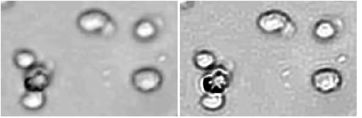
Figure 3.3: No neighbors results: original vs. processed.

In the figure3.3we have the original image (on the left) and the processed image (on the right), using σ = 12 and the weighting variable = 0.8. As shown, the processed image reveals improved contrast.

(34)

3.1.3 Nearest neighbors

It’s one of the simplest methods to use and to compute that gathers some of the available 3D information. It processes a plane z by blurring it’s neighbor planes z ± 1 - hence the name nearest neighbors - and subtracting the blurred planes from z [8,20]:

fs(x, y) = fz(x, y) − c[ fz−1(x, y)gz−1(x, y) + fz+1(x, y)gz+1(x, y)], (3.6)

where the subscript z indicates the optical slice number. One 2D image is sharpened at a time, with the neighboring images immediately above and below it blurred the same way as in the no neighbor methods, and a fraction c of them subtracted out [21].

A 3D stack of images is processed by applying the algorithm to every plane in the stack where, from each plane, an estimate of the blur is removed. Nearest neighbor methods work best when the amount of blur from one plane to the next is significant. Since the algorithms involve relatively simple calculations on single image planes, they are also most useful in situations when quick image sharpening is needed and computing power is limited. The advantages of this approach include computational speed, improved contrast, and sharpening of features in each optical slice.

Each 2D image in a 3D stack contains information from the corresponding in focus specimen plane plus a sum of defocused adjacent specimen planes. It is possible to par-tially remove defocused structures by subtracting adjacent plane images that have been blurred by convolution with the appropriate defocus PSF. In the nearest neighbor method only two immediately adjacent planes are used, one above the plane of focus and the other below. While the image taken at any one focal plane actually contains out of focus light from all specimen planes, the nearest neighbor method assumes that the strongest contributions come from the nearest two adjacent planes [19].

There are also several disadvantages to this approach. These methods are sensitive to noise and may produce noisier images, since noise from several planes tends to get added together. They also tend to introduce structural artifacts because each optical slice may contain diffraction rings or light from other structures that may be sharpened as if it were in that focal plane.

3.1.3.1 Nearest neighbors processing

In the nearest neighbors algorithm we must set the σ value and the weighting parameter’s value like we did in no neighbors. Though both methods require the same parameters, the process is different as nearest neighbors works with one more z plane than the no neighbors. The range of values of σ goes the same as for the no neighbors, creating a “halo” effect if the value is improper, i.e., if it exceeds the limits mentioned - 4 to 12 pixels.

(35)

The weighting parameter’s value has a different range as this algorithm subtracts two adjacent images to the image being processed. This means that an improper weighting value removes too much information and therefore its range must be lower in order to achieve good imaging results. The weighting parameter works better with values between 0.2 and 0.5 and the results are cleaner than the no neighbors. The output image is com-posed of high frequencies and different objects among the adjacent images, as seen below:

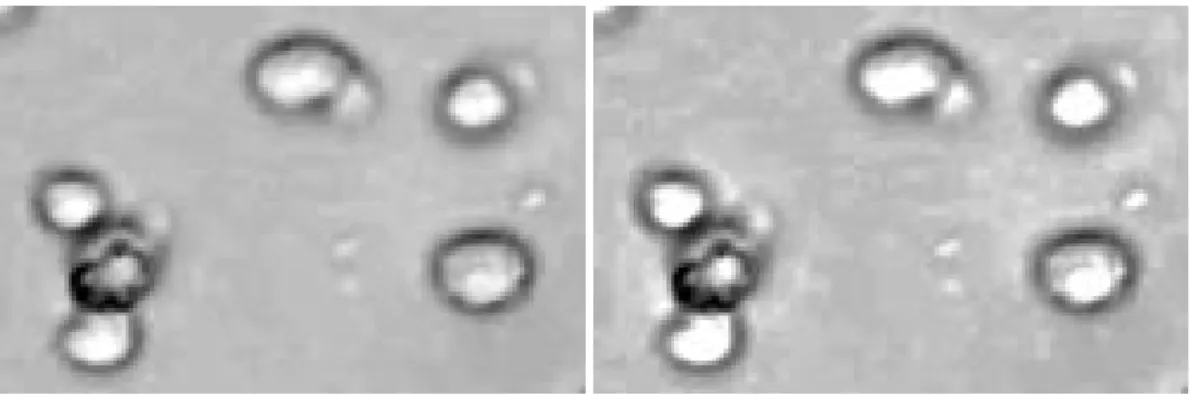
Figure 3.4: Nearest neighbors results: original image versus processed.

Figure3.4reveals the original image versus the processed one. We used σ = 12 and c = 0.3.

3.1.4 Linear deconvolution

Linear methods represent one of the simplest 3D methods for deconvolution. These meth-ods attempt to directly solve the imaging equation3.1described above using the informa-tion from all focal planes. This is achieved in the frequency domain by converting into a multiplication in the Fourier domain, allowing us to solve for S, as follows:

F (S) = _{F (PSF)}F (I) , (3.7)

whereF represents the Fourier transform operator.

The computation is as fast as the 2D deblurring methods discussed above. However, this method is limited by noise amplification. During division in Fourier space, small noise variations in the Fourier transform are amplified by the division operation. The result is that blur removal is traded against a gain in noise. As a result, artifacts like “ringing” effects can be introduced to the objects [16].

Both noise amplification and ringing artifacts can be reduced by making some as-sumptions about the structure of the object that gave rise to the image. For instance, if we assume that the object was relatively smooth, we can eliminate noisy solutions with rough edges - this is called regularization. A regularized inverse filter can be thought of

(36)

as a statistical estimator that applies a certain kind of “constraint” on possible estimates, given some assumption about the object. A constraint on some assumption enables the algorithm to select a reasonable estimate out of the large number of possible estimates that can arise due to noise variability.

The implemented approach is similar to the Wiener method and preprocesses each image of the stack (2D) or the whole stack (3D):

F (S) = _|_{F (PSF)}F (PSF)F (I)₂_|_{F (I) + N}. (3.8) Regularization can be applied in one step within an inverse filter or it can be applied iteratively [22]. It’s possible to regularize the equation in order to consider the influence of noise. To do that we just add the noise component (N(X ,Y, Z)) to the image equation3.1

and then invert the equation, solving for S - see equation3.8.

In image processing software, these algorithms go by a variety of names including “Wiener deconvolution”, “regularized least squares”, “linear least squares” and “Tikhonov-Miller regularization” [10,19,23,24].

The result is usually smoothed, i.e., stripped of higher Fourier frequencies. Much of the “roughness” being removed occurs at Fourier frequencies well beyond the resolution limit and therefore does not eliminate structures recorded by the microscope. However, since there is a potential for loss of detail, software implementations of inverse filters typically include an adjustable parameter which allows the user to control the tradeoff between smoothing and noise amplification [10].

3.1.4.1 Linear deconvolution processing

We can apply this methodology to 2D as well as 3D analysis.

As seen, linear deconvolution is the simplest form of deconvolution. The way it pro-cesses images is completely different from the above methods described. It works on the frequency domain and considering a PSF. The difference between 2D and 3D linear de-convolution has to do with the way it considers the input images and how it works with the PSF, as both implementations follow the regularized equation3.8. In the 2D decon-volution, the input is a 2D image with a 2D PSF defined by a Gaussian function with a certain radius and σ . In the 3D deconvolution, the algorithm considers the entire stack of images and the PSF is a 3D distribution affecting every point of the stack like two inverted cones.

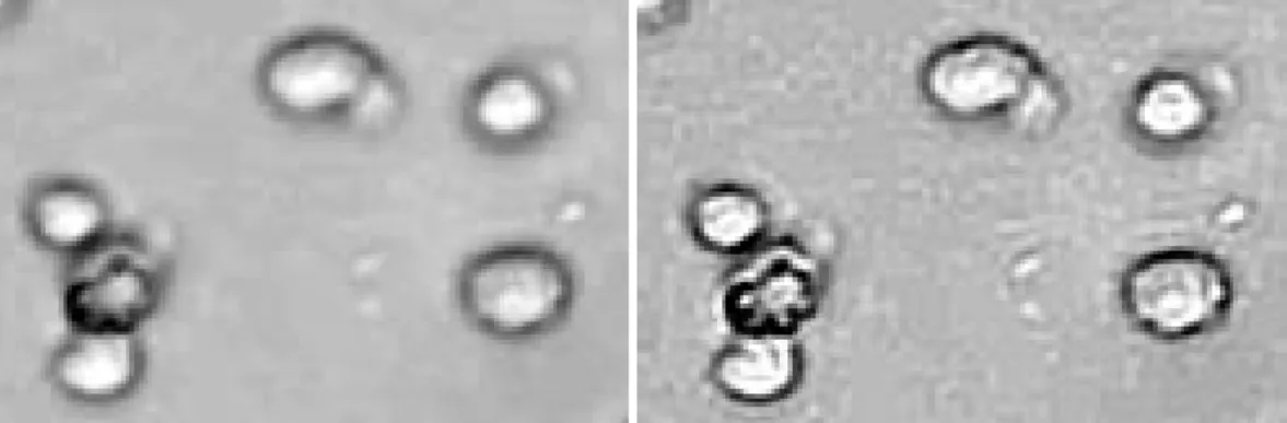
For the 2D linear deconvolution, the best results were imaged using σ = 1.4, as seen in figure 3.5. Although this value appears to be very low, setting σ with higher values results in loss of definition.

By inspecting images from both methods we can see the 3D linear deconvolution yields better results by providing better contrast images with less blur.

(37)

Figure 3.5: 2D Linear deconvolution results: original image versus processed.

(38)

3.1.5 Blind deconvolution

No matter how good the preceding deconvolution methods are, if they are given an in-accurate PSF the deconvolved image will suffer. Noise is always introduced in a PSF measurement and even if a theoretical PSF is used, it cannot completely account for aber-rations present in any optical system.

Blind deconvolution is a relatively new method that greatly simplifies the use of de-convolution for the non-specialist. It was developed by altering the maximum likelihood estimation algorithm so that not only the object, but also the PSF is estimated [16,21].

In this approach, an estimate of the object is made and convolved with a theoretical PSF calculated from optical parameters of the imaging system. The resulting blurred estimate is compared with the raw image, a correction is computed, and this correction is used to generate a new estimate. This same correction is also applied to the PSF, generating a PSF estimate. In further iterations, the object estimate and the PSF estimate are updated together using the equations below [21].

Ob ject estimate: ˆf_i+1k (x, y, z) = g(x, y, z) ˆ f_ik(x, y, z)ˆhk−1(x, y, z)ˆh k−1_{(−x, −y, −z) ˆ}_fk i(x, y, z), (3.9) PSF estimate: ˆhk_i+1(x, y, z) = g(x, y, z) ˆhk i(x, y, z) ˆfk−1(x, y, z) ˆ fk−1(−x, −y, −z)ˆhk_i(x, y, z). (3.10)

A possible approach is to constrain the PSF to be circularly symmetric and band-limited [21]. Another approach is to apply a quadratic parameterization to enforce non-negativity on f and use a PSF parameterization based on phase aberrations in the pupil plane for h.

However, less information is supplied to solve the deconvolution problem and as it’s also iterative so it becomes a time consuming method.

Blind deconvolution methods take twice as long per iteration as the maximum likeli-hood technique because two functions (i.e., object and PSF) are being estimated. They can produce better results than using a theoretical PSF, especially if unpredicted aber-rations are present. The algorithm adjusts the PSF to fit the data and can thus partially correct for spherical aberration [10,16,21,25].

In short, blind deconvolution methods work well not only on high-quality images, but also on noisy or spherically degraded images. Though it begins with a theoretical PSF adapts it to the specific data being deconvolved. As an advantage, it spares the user from the difficult process of acquiring a high-quality empirical PSF.

(39)

3.2 Cell detection algorithm 21

3.1.5.1 Blind deconvolution processing

The blind deconvolution method, though implemented as a 2D algorithm, provides good high contrast images like both linear deconvolution methods. However, depending on the settings we selected, while being able to adapt the object and the PSF on every iteration, we noticed that if the value for the Gaussian’s σ is bigger than 1.4 and the number of iterations is bigger than 15, images start to loose definition and a “ringing” effect starts appearing. Nevertheless, blind deconvolution seems to be a good choice for general de-convolution procedures as it doesn’t depend on the inputed PSF to generate good results.

Figure 3.7: Blind deconvolution results: original image versus processed.

3.2 Cell detection algorithm

The detection algorithm determines the position of the in-focus cells per image.

The identification works by performing a phase symmetry detection on images to detect the walls of the cells - this method seeks for objects or local areas with some degree of symmetry in images, like the external structure of the cells for their ridged form. After finding the cell’s walls, an Hough transform algorithm is performed to detect circle-shaped objects. The Hough transform locates the in-focus cells shapes based on the form and intensity of the phase symmetry results. By using the results of the Hough transform over the phase symmetry information we get the locations of the highest detected in-focus cells present in the images.

We’ll start by describing the phase symmetry followed by the Hough transform.

(40)

The phase symmetry algorithm searches for ridges in images by the analysis of local frequency/phase information. As the external structures of cells are symmetric, the results of this method against the results of edge detecting methods like Sobel, Prewitt or Canny, proved to be very efficient.

The phase information can be used to construct a contrast invariant measure of sym-metry that does not require any prior recognition or segmentation of objects. Under the most general definition of symmetry an object is considered symmetric if it remains in-variant under some transformation.

An important aspect of symmetry is the periodicity that it implies in the structure of the object that one is looking at. Accordingly it’s perhaps natural that one should use a frequency based approach in attempting to recognize and analyze symmetry in images.

In this work the wavelet transform is used to obtain local frequency information [26]. The basic idea behind wavelet analysis is that one uses a bank of filters to analyze the signal. The filters are all created from rescalings of the one wave shape, each scaling designed to pick out a particular band of frequencies from the signal being analyzed. An important point is that the scales of the filters vary geometrically, giving rise to a logarithmic frequency scale. As we’re interested in the calculations of local frequency and phase information from signals, linear-phase filters must be used in order to preserve phase information, i.e., we must use wavelets that are in symmetric/anti-symmetric pairs. For further details on the subject consult Kovesi’s work [27].

The results obtained from the phase symmetry measure can sometimes have no ap-parent logic in a image context as this method measures local symmetry to the exclusion of everything else. The measure is invariant to the magnitude of the local contrast and so features that we might consider to be of little significance can be marked as having strong symmetry (see Figure3.8).

Summing up, local symmetry in image intensity patterns can be identified as being particular arrangements of phase that arise at these points. The phase symmetry algo-rithm used here is considered a low-level operator that does not require any prior object recognition or segmentation. It’s dimensionless measures provide an absolute sense of the degree of local symmetry or asymmetry independent of the image illumination or contrast.

Below, the phase symmetry algorithm on an example cell from an image of the stack in use.

3.2.2 Hough transform

The Hough transform is used for identifying the locations and orientations of certain types of features in an image. A big advantage of this approach is the robustness of the

(41)

3.2 Cell detection algorithm 23

Figure 3.8: Phase symmetry detection: original, phase symmetry (from left to right).

algorithm to imperfect data or noise.

In theory, it can be used to find features of any shape in an image. In practice it is only generally used for finding straight lines or circles. The Hough transform is used when an analytical description of the feature we are searching for is not possible. Instead of a parametric equation describing the feature, we use a lookup table, correlating locations and orientations of potential features in the original image to some set of parameters in the Hough transform space [28].

So, the transform consists of parameterizing a description of a feature at any given location in the original image’s space. A mesh in the space defined by these parameters is then generated, and at each mesh point a value is accumulated, indicating how well an object generated by the parameters defined at that point fits the given image. Mesh points that accumulate relatively larger values then describe features that may be projected back onto the image, fitting to some degree the features actually present in the image.

Figure 3.9: Each point in the image space (left) generates a circle in the accumulator space (right). The circles in the accumulator space intersect at the (x, y) coordinates which is the center of the circle in the image space.

As we want to detect circles, let’s consider a dark circle in an image with an uniform bright background like the one on the left side of the figure3.9, where (a, b) is the coordi-nate of the center of the circle that passes through (x, y), being r its radius and described as:

(42)

and

y= b + rsin(θ ). (3.12)

The method starts with a search for dark image pixels sweeping the angle θ through the full 360 degree range. After finding the points (x, y) belonging to the perimeter of the circle, a locus of potential center points, in the accumulator space, forms a circle with the radius r, as demonstrated in Figure3.9on the right).

Let’s suppose the image contains many points, some of them in the perimeter of the circle; then the job of the algorithm is to find parameter triplets (a, b, r) to describe each circle. The fact that the accumulator space is 3D, makes a direct implementation of the Hough technique more expensive in computer memory and time. If the circles in an image are of known radius r, then the search can be reduced to 2D. The objective is to find the (a, b) coordinates of the centers in the accumulator space. The locus of (a, b) points in the accumulator space fall on the perimeter of a circle of radius r centered at (x, y), making of this (x, y) coordinate the true center point common to all the parameter circles in the accumulator space. The intensity of a pixel is determined by the number of votes it gets in the accumulator space [28,29].

Below, a representation of the Hough transform detection of the center of a in-focus cell.

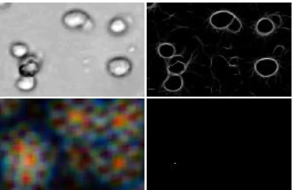
Figure 3.10: Hough transform: original, phase symmetry, Hough transform accumulator space and the representation of the maximum Hough detected point (from left to right, top to bottom).

(43)

3.3 Depth estimation 25

After the detection is computed, the identified in-focus cells are marked with a green circle with a radius equal to the radius value inputted in the Hough transform algorithm for the detection - figure3.11.

Figure 3.11: Cell detection: original image on the left and detected cell image on the right.

3.3 Depth estimation

Depth estimation methods allow the determination of the depth cells reached in the assay. To be able to quantify this vertical extent, we developed two methods that work by estimating the focus measure of cells from each z plane. The first method is based on focus estimation methods using a Laplacian operator that analyses the focal distance of the cells to the focus plane and the second was implemented using the Hough transform method to detect the depth of cells by their intensity per z plane. These methods work one cell at the time and we’ll present both in the following subsections - subsections3.3.1and subsections3.3.2.

3.3.1 Focus estimation using Laplacian

The objective of shape from focus is to estimate the focal distance of each point in the image to the camera.

This method uses a depth map to recover 3D shape of the object [30]. A sharp image and the relative depth can be retrieved by collecting the best focused points in each image. The absolute depth of object surface patches can be calculated from the focal length and the position of lens that gave the sharpest image of the surface patches. The depth or best focus is obtained by using focus measures.

Every shape from focus method relies on a focus measure operator and an approxima-tion technique. Focus measure operator plays a very important role for three dimensional shape recovery because it’s the first step in the calculation of the depth map.

(44)

Every point’s depth is calculated by the determination of the best focused points, i.e., sharpest pixel values. Hence the operator should produce high response to high frequency variations of the image intensity, since better focused images have higher frequency com-ponents [31]. A focus measure operator should provide a good estimate of the depth map by showing robustness even in the presence of noise.

Shape from focus can be implemented through different focus measure operators such as Laplacian [32] and modified Laplacian [32,33], sum of the modified Laplacian, Tenen-baum [34], gray level variance focus measure [34], mean method focus measure [34] and curvature focus measure [34] as well as approximation methods like Gaussian interpola-tion, neural networks, dynamic programming, etc., though we’ll only explore Laplacian in this report.

3.3.1.1 Laplacian operator

The Laplacian operator, being a point and symmetric operator, is suitable for accurate shape recovery. If I(x, y) represents an image frame, then this focus measure is obtained by adding second derivatives in the x and y directions, such that:

∇2I(x, y) =∂

2_{I(x, y)}

∂ x2 +

∂2I(x, y)

∂ y2 . (3.13)

In applications where computation needs to be minimized by computing only one focus measure, it is recommended to use the Laplacian as the focus measure filter. Laplacian has some desirable properties such as simplicity, rotational symmetry, elimination of un-necessary information, and retaining of un-necessary information. Laplacian is computed for each pixel of the given image window and the criterion function can be stated as:

∑

x

∑

y

∇2= I(x, y). (3.14)

Above we have an example of a cell depth estimation using the Laplacian operator. As seen in the figure, using a stack with 13 images, the cell is located at the equivalent depth of the ninth plane in the z axis.

3.3.2 Hough response based estimator

This method works the same way as the detection algorithm described in the section3.2 -Cell detection algorithm. Being an intensity response based estimator, the values of signal strength can’t be compared to the Laplacian’s.

In this example using the Hough response based algorithm, in the same stack with 13 images, the cell is detected at the equivalent depth of the eighth plane in the z axis.

(45)

3.3 Depth estimation 27

(46)

(47)

Chapter 4

Results discussion

In this chapter we’ll analyze and present the results of the methods described in the last chapter.

We’ll start by presenting the deconvolution algorithms with their results for a sam-ple section of the images from the stack, as doing so permits a better visualization, and therefore a better comparison of the methods.

The results of the deconvolution algorithms will be posteriorly used to verify their influence on the detection algorithm identification of in-focus cells. What matters in this section is the analysis evaluation of the deconvolution methods to help to determine in-focus cells.

After the deconvolution and the detection algorithms, we’ll discuss the depth estima-tion results, comparing the evaluaestima-tions done by each method about the depth of the cell being analyzed.

4.1 Analysis of the deconvolution methods

In this section we’ll be showing raw images of the stack against the images from each method.

4.1.1 No neighbors analysis

By observing the images we notice changes are few from the original to the deblurred image. This method has a poor contrast definition that is justified by its simple algorithm basis.

(48)

30 Results discussion

(49)

4.2 Analysis of the detection methods 31

4.1.2 Nearest neighbors analysis

Let’s now consider nearest neighbors. These method brings a new plane in the deblurring field permitting better results than the no neighbors at the same computational expense and speed. It exhibits better contrast but it’s at the same time prone to loose high frequency information if the weighting value is not chosen correctly.

4.1.3 Linear deconvolution analysis

This is so far the first real deconvolution method as it works considering the imaging equation3.1. Actually, to be able to perform the linear deconvolution on images, one must regularize the algorithm because of the presence of noise. Our regularization approach was based on the Wiener filter - see equation 3.8. This method improves the image by deblurring it and improving the overall contrast in all the images.

We also implemented a 3D linear regularized deconvolution algorithm for testing pur-poses and the results were very satisfactory, as seen in the image4.4.

4.1.4 Blind deconvolution analysis

The blind deconvolution method presented in figure 4.5 demonstrates very good results considering that is a method that iteratively keeps upgrading the object and the PSF. The deblurring results and the contrast improvement is similar to the results we have from linear 2D deconvolution, which makes it a very powerful algorithm considering that it doesn’t completely depend on the PSF to achieve the results linear did.

4.2 Analysis of the detection methods

In this section we’ll show raw images of the stack with the resulting images from each method where the detection algorithm is applied onto.

4.2.1 Detection algorithm analysis

Considering that both no neighbors ( 4.6) and nearest neighbors ( 4.7) are deblurring algorithms, is no surprise the detector performs the same identification on them as they don’t differ too much on the way of altering the image. On the other hand, both influence the identification on a cell that no other deconvolution method lead the detector to identify. With that said, in our sample image, both linear deconvolution methods inhibited the detection algorithm of identifying the same cell that the detector found after being pre-ceded by the deblurring algorithms - same goes for the detection after blind deconvolution. Detection after blind deconvolution shows an identification of another possible in-focus cell.

(50)

(51)

(52)

(53)

(54)

4.3 Analysis of the depth estimation methods

In this section we’ll expose the detections from both methods: Laplacian focus estimation and Hough response based estimation. The methods took the input stack of images like the one presented in figure4.11.

4.3.1 Laplacian focus estimation analysis

As observed in figure 4.12, the estimation of the Laplacian operator shows that the cell is best focused around the ninth optical slice. While being a good estimative the truth is we can’t completely rely on this approach as it’s the only method of focus estimation operators we computed.

4.3.2 Hough response based estimation analysis

While observing the image 4.13 we verify that the detection done by this algorithm is different than the Laplacian’s. In this approach, the result indicates the cell is best focused, and therefore, at an equivalent depth to the z axis value indicated as eithth.

Comparing both graphics we can tell the significance of the values of intensity credits the Hough response based estimator though we can’t fundament our statement on this values.

Therefore, we computed the five previously described deconvolution methods on the images and applied the Hough estimator on them. The result is represented in figure4.15. In conclusion, performing all these variations, the Laplacian’s estimation is for the ninth image while the linear 2D deconvolution detects the seventh for the depth from focus analysis. All the other methods yield the eighth image as the closest to the cell being analyzed.

(55)

4.3 Analysis of the depth estimation methods 37

Figure 4.6: No neighbors results: original vs. deblurred.

(56)

Figure 4.8: Linear 2D deconvolution results: original vs. deconvolved.

(57)

Figure 4.10: Blind deconvolution results: original vs. deconvolved.

(58)

(59)

(60)

(61)

(62)

(63)

Chapter 5

Conclusions

As seen in this work, the detection of cell’s invasion using microscopy images is com-posed of three main steps: image deconvolution, cell detection and depth estimation.

The image improvements either by enhancement or deblurring algorithms take a se-quence of trial and error procedures that must be considered.

We took deconvolution as the method to improve our image’s contrast and to removes the haze caused by the out-of-focus light but its results don’t always succeed, varying from case to case.

Each deconvolution method has it’s advantages and disadvantages being that the most faithful methods to the concept of deconvolution deliver better results. The differences have been pointed out throughout the work and the final conclusions about the deconvo-lution methods are related to the need of having a good estimate of the PSF and negative influence of noise in images for deconvolution. The absence of a good PSF estimative and noisy images reduce the room to improvements achieved by the deconvolution methods.

As we couldn’t have the detection algorithm biased by any means, the difference of the results it’s therefore attributed to the deconvolution methods per se. There’s still room for improvements and the outcomes achieved satisfactory levels of result.

The detection algorithm proved to be an all around good performer as it accomplished the task of acting as a detection method to determine the in-focus cells in the image’s stacks and as a response based estimator capable of being compared with a focus estimator operator for determination of relative depth.

Though there were some discrepancies on the depth estimation results, the overall detection methods achieved satisfactory levels of identification for the images in use.

In general, the work evolved as planned and the objectives were accomplished in time. As a development work, we’ll keep the process of validating data till the final report period.

(64)

(65)

References

[1] P. Sarder and A. Nehorai. Deconvolution methods for 3-d fluorescence microscopy images. IEEE SIGNAL PROCESSING MAGAZINE, Vol. 23, Issue 3, pages 32–45, May 2006.

[2] World Health Organization. Cancer - fact sheet no297, February 2009. http: //www.who.int/mediacentre/factsheets/fs297/en/.

[3] Eric A. Bruyneel Marc E. Bracke, Tom Boterberg and Marc M. Mareel. Collagen Invasion Assay, Methods in Molecular Medicine , vol 58. Academic Press, 1999. [4] J. B. Pawley. Handbook of Biological Confocal Microscopy. Springer, 2006. [5] C. J. R. Sheppard and D. M. Shotton. Confocal Laser Scanning Microscopy.

Springer, 1997.

[6] S. Inoue and K. R. Spring. Video Microscopy: The Fundamentals. Plenum, 1997. [7] D. Semwogerere V. Prasad and Eric R. Weeks. Confocal microscopy of colloids.

Journal of Physics: Condensed Matter, Vol. 19, pages 113–102, 2007.

[8] D. A. Agard. Optical sectioning microscopy: Cellular architecture in three dimen-sions. Ann. Rev. Biophys. Bioeng., Vol. 13, pages 191–219, 1984.

[9] M. Abramowitz and M. W. Davidson. Introduction to microscopy, 2007.

[10] J. Cooper J.G. McNally, T. Karpova and J. A. Conchello. Three-dimensional imag-ing by deconvolution microscopy. Methods, Vol. 19, Issue 3, pages 373–385, November 1999.

[11] J. L. Arauz-Lara J. Baumgartl and C. Bechinger. Like-charge attraction in confine-ment: myth or truth ?, May 2006.

[12] T. J. Fellers S. W. Paddock and M. W. Davidson. Confocal introductory concepts. [13] Richard E. Woods and Rafael C. Gonzalez. Digital Image Processing. Prentice Hall,

1992.

[14] I. J. D. Craig and J. C. Brown. Inverse problems in astronomy: a guide to inversion strategies for remotely sensed data, 1986.

[15] S. L. Moltz T. S. Karpova, J. G. McNally and J. A. Cooper. Assembly and function of the actin cytoskeleton in yeast: relationships between cables and patches. J. Cell Biol., Vol. 142, Issue 6, pages 1501–1517, September 1998.

(66)

48 REFERENCES

[16] W. Wallace J. Swedlow and L. H. Schaefert. A workingperson’s guide to deconvo-lution in light microscopy. BIOTECHNIQUES, 2001.

[17] Scientific Volume Imaging. Point spread function.

[18] T. J. Keating J. R. Monck, A. F. Oberhauser and J. M. Fernandez. Thin-section ratiometric ca2+ images obtained by optical sectioning of fura-2 loaded mast cells. J. Cell Biol., Vol. 116, Issue 3, pages 745–759, February 1992.

[19] K. R. Castleman. Digital image processing. Prentice-Hall, 1979.

[20] M. Weinstein and K. R. Castleman. Reconstructing 3-d specimens from 2-d section images. Proceedings of the Society for Photo-Optical Instrument Engineering, 26, pages 131–138, 1971.

[21] Kenneth R. Castleman Fatima A. Merchant and Qiang Wu. Microscope Image Pro-cessing. Academic Press, April 2008.

[22] C. Preza et al. Regularized linear method for reconstruction of three-dimensional microscopic objects from optical sections. J. Opt. Soc. Am. A., Vol. 9, Issue 2, pages 219–228, 1992.

[23] D. Shotton. Computer reconstruction in three-dimensional fluorescence microscopy, P. J. Shaw. John Wiley and Sons, 1993.

[24] A. N. Tikhonov and V. Y. Arsenin. Solutions to ill-posed problems. Bull. Amer. Math. Soc. (N.S.) Vol. 1, Number 3, pages 521–524, 1979.

[25] J. B. Pawley. Light microscopic images reconstructed by maximum likelihood de-convolution, T. J. Holmes et al. Plenum Press, 1995.

[26] J. Morlet et al. Wave propagation and sampling theory - part ii: Sampling theory and complex waves. Geophysics, Vol. 47, Issue 2, page 222–236, February 1982. [27] Peter Kovesi. Symmetry and asymmetry from local phase. In Proceedings of the

Tenth Australian Joint Conference on Artificial Intelligence, pages 185–190, Decem-ber 1997.

[28] Vaclav Hlavac Milan Sonka and Roger Boyle. Image Processing, Analysis and Ma-chine Vision. Thomson-Engineering, 2007.

[29] P. V. C. Hough. Method and means for recognizing complex patterns. Technical report, 1962.

[30] Seong-O Shim A.S. Malik and Tae-Sun Choi. Depth map estimation using a ro-bust focus measure. IEEE International Conference on Volume 6, pages 564–567, September 2007.

[31] Tarkan Aydin and Yusuf Sinan Akgul. A new adaptive focus measure for shape from focus. British Machine Vision Conference, 2008.

[32] S.K. Nayar and Y. Nakagawa. Shape from focus: An effective approach for rough surfaces. In Proceedings of 1990 IEEE International Conference on Robotics and Automation, Vol. 2, pages 218–225, May 1990.

(67)

REFERENCES 49

[33] S.K. Nayar and Y. Nakagawa. Shape from focus. IEEE Transactions on Pattern Analysis and Machine Intelligence, Vol. 16, Issue 8, pages 824–831, August 1994. [34] F. S. Helmli and S. Scherer. Adaptive shape from focus with an error estimation in

light microscopy. In Proceedings of the 2nd International Symposium, pages 188– 193, June 2001.

Development of bioinformatics tools to track cancer cell invasion using 3D in vitro invasion assays

F

E

U

P

Development of bioinformatics tools to

track cancer cells invasion using 3D in

vitro invasion assays

Rui Sérgio Malheiro Caldeira

Development of bioinformatics tools to track cancer cells

invasion using 3D in vitro invasion assays

Rui Sérgio Malheiro Caldeira

Report of Project/Dissertation

Integrated Master in Electrical and Computer Engineering

Approved in oral examination by the committee:

Resumo

Abstract

Acknowledgments

Contents

List of Figures

Abbreviations and Symbols

Chapter 1

Introduction

Chapter 2

Microscopy

2.1

Confocal

2.2

Brightfield

2.3

Confocal vs Brightfield

Chapter 3

Image deconvolution, cell detection and

depth estimation

3.1

Image deconvolution

3.2

Cell detection algorithm

3.3

Depth estimation

∑

∑

Chapter 4

Results discussion

4.1

Analysis of the deconvolution methods

4.2

Analysis of the detection methods

4.3

Analysis of the depth estimation methods

Chapter 5

Conclusions

References