Herding through the tails?

(1)

Herding through the tails?

André Santos Pinto

152110004

Abstract

This paper investigates institutional herding for extreme event-days in the US stock market between 2000 and 2010. We show that, for more extreme return’ stocks, abnormal returns and abnormal turnover are strongly linked to institutional ownership. Six month post-event performance show evidence of overreaction and underreaction by institutions on the event-days, consistent to findings related to informational cascades and the uncertain information hypothesis.

Professor José Faias Supervisor

Dissertation submitted in partial fulfillment of the requirements for the degree of MSc in Business Administration, at Universidade Católica Portuguesa, September 2012.

(2)

(3)

Acknowledgments

Foremost, I would like to express my most sincere gratitude to my supervisor, Professor José Faias. Without his continuous support, his motivational strength, his share of knowledge and his patience, this master thesis could not have been done. I could not be more grateful to him.

Besides my supervisor, I have to thank to my girlfriend Carlota that was there for me at all time; my parents to allow me to study what I love; my friends Miguel, Ana, João, Marta, Pedro, Daniela, Paulo, Claudio, Gonçalo, Luís and Francisco; my colleagues at Banco BPI; my colleagues of the Empirical Finance seminar; my beloved family for their unconditional support.

Last but not least, I have to give a special acknowledge to Fundação para a Ciência e Tecnologia (FCT) and Católica-Lisbon Research Unit for all the support.

(4)

Index of Tables

Table I - Extreme Days’ Market Returns 4

Table II - Event-Day Descriptive Statistics – All stocks 7

Table III - Event-day Adjusted market Return Regression – All stocks 10

Table IV - Event-Day Abnormal Turnover Regression – All stocks 14

Table V - Post-event Performance Statistics – All stocks 17

Table VI - Event-Day Descriptive Statistics – Extreme Stock Returns 21

Table VII - Event-day Adjusted market Return Regression – Extreme Stock Returns 22

Table VIII - Event-Day Abnormal Turnover Regression – Extreme Stock Returns 25

Table IX - Post-event Performance Statistics – Extreme Stock Returns 26

Index of Figures

Figure 1 - Unconditional event-days 4

Figure 2 – Evolution of total, domestic and foreign institutional ownership

between 2000 and 2010 5

(6)

(7)

I. Introduction

De Bondt and Thaler (1985) find evidence that investors overreact to both bad and good news. As a consequence to this overreaction, past losers become underpriced and past winners become overpriced. Jegadeesh (1990) and Lehmann (1990) show that by using “contrarian strategies” in a short-term period, it is possible to have exceptionally large returns, which can outperform the market. These strategies are transaction intensive and their performance could be due to lack of liquidity in the market or the presence of short-term price pressure rather than overreaction. Others like Shefrin and Statman (1985), Lehman (1990) and Goetzmann and Massimo (2002) also show how buying past losers, or selling past winners consistently leads to very positive returns. While the former find empirical evidence with holding periods of 3 to 5 years, Jegadeesh (1990) and Lehmann (1990) bump into the same conclusion but find evidence of overreaction in shorter periods (months and weeks). Evidence of overreaction is also examine in other markets. Schiereck, De Bondt, and Weber (1999) examine contrarian strategies for companies listed on the Frankfurt stock exchange and their results show that implementing these contrarian strategies outperform a passive approach. The same results are obtained for the Japanese stock market (Chang et al. (1995)), for the Chinese Stock market (Kang et al. (2002)), for the Malaysia market (Hameed and Ting (2000) and for the Korean markets (Chui et al. (2000)).

Dennis and Strickland (2002) (henceforth DS) analyzes who is responsible for this overreaction. They consider two types of investors, institutional and individuals. The importance of institutions on the equity markets have been growing for the past few decades. Institutional ownership (IO) is the percentage of capital owned by institutions such as banks, insurance companies, pension funds, endowments and mutual funds. According to Jiang (2010), at the end of 2004, institutional investors hold 53% of the US equity market, a significant increase from the 20% that was registered in 1980. At the end of 1989, institutions were responsible for 70% of the trading volume (Schwartz and Shapiro (1992)) whereas in 2002 they were already responsible for 96% of the volume trade on the NYSE (Jones and Lipson (2004)).

There is a strong positive relation between institutional trading and stock returns, suggesting that institutional investors herd together and trade with the momentum (Nofsinger and Sias (1999); Cai, Kaul, and Zheng (2000); Sias, Starks, and Titman (2001)). Under this

(8)

premise, that institutional investors herd when there is a large drop or a large increase on the market, it can be concluded that they are moving stock’s prices away from their true value (Scheinkman and Xiong (2003)) and if that is so, the market will be forced to correct them and to move their prices to their fundamental value again. Morris and Shin (1999) and Persaud (2000) argue that herding behaviour creates volatility, destabilize the market and force firms to focus on short-term strategies. If this is true, it is possible to take advantage of this situation.

We follow Dennis and Strickland (2002). We use US stock data between 2000 and 2010 to test if institutional investors are herding during days with extreme returns. We make several contributions. First, we enlarge the sample size of extreme returns due to the choice of the period of time. Second, this is a more recent period of time and the previous results could not hold. Third, we use two methodologies to study this effect. These show that some stocks, the trendy, have a different pattern from just taking the market as a whole.

We identify two types of event-days, days in which there is a large market drop, down market, and days in which there is a large market increase, up market. We link abnormal stock return and abnormal turnover on each event-day to institutional ownership. If institutional investors are selling (buying) more than individuals in days when there is a large market drop (increase), stocks with higher IO in their capital structure should have more negative (positive) returns since these investors herd and trade with the momentum. Empirical evidence shows that there is some correlation between these two variables, however, the relationship is different from what was expected. If herding is occurring on such extreme days, the empirical evidence suggests that institutions are not contributing for the extreme returns, in fact they are not trading with the momentum but against it. Evidence from the abnormal turnover model also shows that the level of turnover of a stock on the event-day is positively related to the presence of institutions on a stock capital structure suggesting that institutions react strongly to the extreme day.

We analyze post-event performances, six months after the event-day in order to test if institutions are overreacting to the event-day and deviating stock’s prices away from their true value. Post-herding returns reveal evidence of underreaction (overreaction) for the up (down) market event-days. These results are consistent in accordance to Schnusenberg and Madura (2001) and Lasfer, Melnik and Thomas (2003). The results for the up market event-days are also consistent with evidence from several authors that suggest that institutional herding may

(9)

not be related to information, but rather it may be just a result from irrational psychological factors that cause price bubbles (Dreman (1979) and Friedman (1984)).

The remainder of the paper is organized as follows. Section II explains the data and methodology. Section III and IV present our empirical findings for all stocks in the market and for the trendy extreme stocks, respectively. Section V presents the concluding remarks.

II. Data and Methodology

The stock return data consists of 3,422 stocks of Nasdaq and NYSE between January 1, 2000 and December 31, 2010 from Bloomberg. We are limited in our sample to the IO availability data that is obtained through Factset/Lionshares database. This period implies a larger sample of extreme return stock market days. We define the market return to be the equal-weighted average of all stocks in each day.

In order to find the event-days, the market return is compared against its unconditional eleven-year average. We define an (a) up (down) market event-days as a day when the market return is two standard deviations above (below) its unconditional average. Table I contains some of the dates and market returns of those event-days for exemplification.1

Between 2000 and 2010 there are 60 up market event-days, with an average return of 4.24% and 68 down market event-days with an average return of -4.54%. To check if the general trend in the market was reflected on these event-days for most of its individual stock, the percentage of positive, negative and zero-return firms is computed. We also compute the ratio of positive (negative) return firms to negative (positive) return firms for the up (down) market event-days. Large positive or negative returns for a small number of firms could produce an extreme market return when in fact the trend was to have returns with the opposite sign. For the up market event-days, the minimum percentage of positive firms is 67.17%, with a correspondent ratio of 2.64, which is registered on April 18, 2000. On May 27, 2010 it is registered the largest percentage of positive firms, 93.17%, with a correspondent ratio of 15.40. The average ratio for the up market event-days is 6.24, which means that on average there are 6 times more companies with positive returns than firms with negative returns. The trend is similar to the down market event-days, with an average ratio of 8.88. The smallest percentage of negative firms for these days is 71.80% with a ratio of 3.42, registered on

(10)

Table I

Extreme Days’ Market Returns

This table presents a list of some of the event-days with dates, mean returns (%), percentage of firms with positive, negative, and zero returns. The ratio for up market event-days is the ratio of percent positive to percent negative while for down market event-days is the ratio of percent negative to percent positive. The mean return represents the market returns and it is equal to the equal-weighted average of all stocks in the sample from NYSE and Nasdaq.

Date Mean Return (%) Percent Positive Percent Zero Percent

Negative Ratio Date

Mean Return (%) Percent Positive Percent Zero Percent Negative Ratio Panel A: Equal-Weighted Up Event-Days Panel B: Equal-Weighted Down Event-Days 00/03/16 3.05 70.52 6.09 23.39 3.01 00/04/14 -6.24 10.76 5.11 84.14 7.82 00/04/18 4.00 67.17 7.38 25.45 2.64 00/12/20 -3.63 21.02 7.17 71.80 3.42 00/12/05 3.19 69.84 7.81 22.34 3.13 01/03/12 -3.32 13.39 5.70 80.92 6.04 ... ... ... ... ... ... ... ... ... ... ... ... ... ... ... ... ... ... ... ... ... ... ... ... 10/05/10 4.72 93.14 1.10 5.76 16.16 10/06/01 -2.90 9.57 1.05 89.38 9.34 10/05/27 3.81 93.17 0.78 6.05 15.40 10/06/04 -4.28 5.54 1.35 93.11 16.79 10/06/10 3.07 92.02 1.40 6.58 13.98 10/06/29 -3.92 4.26 1.12 94.62 22.21

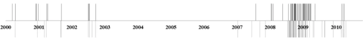
December 20, 2000. On May 20, 2010 the largest percentage of negative firms is registered, 96.12% with a ratio of negative firms of 30.50. When comparing the data sample to DS, the differences are relevant. During their period of analysis (between 1988 and 1996), they register only 6 up event-days and 10 down event-days. The different frequency can be assigned to the financial crisis of 2007. Until 2007, there are only 12 up market event-days and 10 down market event-days. The clustering of these event-days is visible on Figure 1.

Figure 1. Unconditional event-days. Above the timeline are registered the up market event-days and below the timeline are registered the down market event-days.

Our hypothesis is that institutional investors herd and together react to the extreme days. As a consequence, on such event-days, stocks that have more percentage of IO on their capital structure have larger price swings. What this theory implies is that the distribution of returns on such event-days is linked to the level of IO of the firms. If institutions are in fact the cause of this market volatility and if they are only contributing to move stock’s prices away from their true value, the post-event performance will also be linked to the level of IO, once the market is going to correct this overreaction.

(11)

We divide our analysis into two main sections. The first section runs the same framework as DS, but for a different time period. The second section uses only the extreme returns stocks that follow the market.

IO is defined as being the percentage of a firm’s capital that institutions (i.e. banks, pension funds, mutual funds, endowments) hold. The IO is also split into domestic IO (dom

io) and foreign IO (for io). dom io is the percentage of domestic IO on a firm’s capital

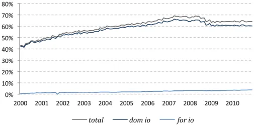
structure and for io is the percentage of foreign IO on a firm’s capital structure. All of the data was obtained through Factset/Lionshares database. Concerning the level of ownership of domestic and foreign investors, it is possible to find huge differences on our sample. Foreign investors still have a very small participation on the US market when compared to domestic ones. The average level of foreign ownership on the event-days is 2.7 and 2.8 percent for up and down market event-days while domestic investors have an average level of ownership on the same event-days of 55.7 and 56.3 percent. Figure 2 shows the differences between the level of dom io and for io in our sample. It is important to note that the level of foreign IO is very low on our sample when compared to previous papers that have analyzed the level of foreign institutions on firm’s capital structure (Ornelas and Alemanni (2008); Chen Yang and Lin (2012)). Note that these previous paper analyse foreign institutional ownership in emerging markets. With this categorization the goal is to understand if the different types of institutions, have different reactions on such event-days. Most of the financial literature highlights the differences between domestic and foreign institutional investors, therefore it is important to try to understand the differences between these two kinds of investors and their impact on our study.

Figure 2. Evolution of total, domestic and foreign ownership between 2000 and 2010.

0% 10% 20% 30% 40% 50% 60% 70% 80% 2000 2001 2002 2003 2004 2005 2006 2007 2008 2009 2010

(12)

Despite the recent trend of globalization and the increase of cross-border investment, foreign investment is still very limited when compared to local investment. French and Poterba (1991), Cooper and Kaplanis (1994), Kang and Stulz (1997) find that the existence of the home bias is still very present and that usually investors tend to overweight their portfolios with domestic firms. Brennan and Cao (1997) attribute this overweight to the difference of information that each of these two types of investors have. Usually foreign investors are less informed. On the other hand, foreign institutions have good resources, not only financial but also human. Grinblatt and Keloharju (2000) even argue that foreign institutions, because of their expertise and local resources can be smarter and more informed than domestic investors. Seasholes (2000) finds evidence that on Taiwan, foreign investors buy stocks ahead of good earnings announcements and sell before the announcement of bad earnings. In contrast, Kang and Stulz (1997) and Coval and Moskowitz (1999) show evidence of better performance by domestic institutions. Another reason that can be attributed to the better performance of domestic institutions is the access to private information. In countries where insider trading can occur, domestic firms will have a better probability to perform better than foreign. The use of this private information will only be seen on a short period of analysis since on the long term the market shall be efficient. But this is not the case for our sample. Another reason to disaggregate into these two types of institution is their strategy style. Choe, Kho and Stulz (1999) and Swanson and Lin (2005) state that foreign institutions have a preference for momentum strategies, buying winners and selling losers.

III. All Stocks

1. Event-Days Descriptive Statistics

The descriptive statistics for the up and down event-days are presented on Panels A and B of Table II, respectively. To explain abnormal returns and abnormal turnover on the event-days, we use the following variables: (a) size, the natural logarithm of the stock’s equity 50 days prior to the event-day; (b) turnover, the daily volume of a stock on the event-day expressed as a percentage of the total number of shares outstanding; (c) variance which is the market model residual variance for the period t-250 days to t-50 days (being t the event-day); (d) beta, the beta of the stocks daily returns with the market return for the period t-250 to t-50; (e) io, the percentage of IO on a firm’s capital structure on the event-day and (f) return, the

(13)

daily return of a firm on the event-day. We also separate higher from lower IO firms. Our results confirms the findings of previous literature. On average, high IO firms are larger than low IO firms (Gompers and Metrick (2001), Bennett, Sias and Starks (2003) and Campbell, Ramadorai and Schwartz (2009)). Firms with lower levels of IO are less liquid than firms with higher levels of IO (Gompers and Metrick (2001), Bennett et al. (2003) and Agarwal (2007)). Firms with more IO on their capital structure have on average lower idiosyncratic volatility but more systematic risk (Brandt, Brav, Graham, and Kumar (2009); Zhang (2010)).

Table II

Event-Day Descriptive Statistics – All stocks

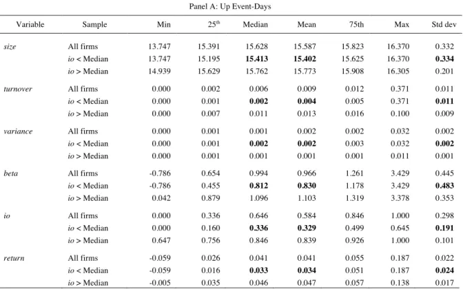
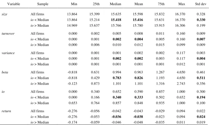
This table presents the descriptive statistics (minimum, first quartile, median, mean, third quartile, maximum, and standard deviation) for the 60 up market event-days (Panel A) and for the 68 down market event-days (Panel B). The event-days are defined as (a) up market, days in which the market return is two standard deviations above its eleven-year average (from 2000 to 2010) and (b) down market, days in which the market return is two standard deviations below its eleven-year average (from 2000 to 2010). Statistics for all firms, and two subsamples, firms with IO below and above the median, are presented. The variables analyzed are size, the natural logarithm of the firm’s equity 50 days prior to the event-day; turnover, the daily volume of a stock expressed as a percentage of the total number of shares outstanding on the event-day; variance, the market model residual variance for the period [-250,-50]; beta, the beta of stocks daily returns with the market return for the period [-250, -50]; io, the percentage of IO on the capital structure of a company on the event-day; and return the daily return of a firm on the event-day.

Panel A: Up Event-Days

Variable Sample Min 25th _Median _Mean _75th _Max _{Std dev}

size All firms 13.747 15.391 15.628 15.587 15.823 16.370 0.332

io < Median 13.747 15.195 15.413 15.402 15.625 16.370 0.334

io > Median 14.939 15.629 15.762 15.773 15.908 16.305 0.201

turnover All firms 0.000 0.002 0.006 0.009 0.012 0.371 0.011

io < Median 0.000 0.001 0.002 0.004 0.005 0.371 0.011

io > Median 0.000 0.007 0.011 0.013 0.016 0.100 0.009

variance All firms 0.000 0.001 0.001 0.002 0.002 0.032 0.002

io < Median 0.000 0.001 0.002 0.002 0.003 0.032 0.002

io > Median 0.000 0.001 0.001 0.001 0.001 0.011 0.001

beta All firms -0.786 0.654 0.994 0.966 1.261 3.429 0.445

io < Median -0.786 0.455 0.812 0.830 1.178 3.429 0.483

io > Median 0.042 0.879 1.096 1.103 1.319 3.378 0.353

io All firms 0.000 0.336 0.646 0.584 0.846 1.000 0.298

io < Median 0.000 0.160 0.336 0.329 0.499 0.645 0.191

io > Median 0.647 0.756 0.846 0.839 0.926 1.000 0.101

return All firms -0.059 0.026 0.041 0.041 0.055 0.187 0.022 io < Median -0.059 0.016 0.033 0.034 0.051 0.187 0.024

(14)

Table II – Continued

Panel B: Down Event-Days

Variable Sample Min 25th Median Mean 75th Max Std dev

size All firms 13.864 15.399 15.635 15.598 15.832 16.370 0.328

io < Median 13.864 15.214 15.418 15.416 15.631 16.370 0.330

io > Median 14.969 15.637 15.766 15.780 15.915 16.306 0.199

io < Median 0.000 0.001 0.002 0.004 0.005 0.160 0.007

io > Median 0.000 0.006 0.010 0.012 0.015 0.099 0.009

io < Median 0.000 0.001 0.002 0.002 0.003 0.117 0.004

io > Median 0.000 0.001 0.001 0.001 0.001 0.012 0.001

beta All firms -0.818 0.631 0.994 0.963 1.267 4.650 0.461

io < Median -0.818 0.429 0.783 0.826 1.193 4.650 0.511

io > Median -0.123 0.873 1.101 1.101 1.316 2.743 0.356

io All firms 0.000 0.340 0.652 0.590 0.857 1.000 0.300

io < Median 0.000 0.166 0.340 0.333 0.502 0.652 0.194

io > Median 0.653 0.764 0.857 0.848 0.935 1.000 0.100

return All firms -0.276 -0.056 -0.042 -0.043 -0.029 0.094 0.022 io < Median -0.276 -0.053 -0.036 -0.038 -0.023 0.094 0.024

io > Median -0.174 -0.059 -0.046 -0.048 -0.035 0.011 0.019

The average beta for the low IO firms is 0.830 and 0.826 for up and down market days, respectively. For high IO firms the betas are 1.103 and 1.101, respectively. The betas between the two subsamples based on IO are statistically different. These results suggest that firms with more IO have their returns’ variations more linked to changes in the market, i.e., firms with more IO are more exposed to extreme market swings. IO statistics is similar for Up and Down event-days. The mean level of IO is around 59% while the median is nearly 65%.2

There is a high level of cross sectional variation. On low IO firms, the first quartile is around 16%, whereas the third quartile is 50%. The high IO firms have a smaller standard deviation, but still considerable cross sectional variation. This heterogeneity is explored in the next section to register different reactions by institutional investors. The median and the average returns are statistically lower for the low IO firms in comparison to high IO firms. There is a higher level of clustering on returns for the high IO firms, reinforcing the idea of herding, i.e., for the high IO firms, that also have higher/lower returns on the up , the value of standard deviation is lower when comparing it to the low IO firms. The high IO firms are also larger and more liquid, which can be the reason for this.

(15)

The next step is to disentangle IO into domestic and foreign. Overall, the descriptive statistics for domestic and foreign IO are similar to those analyzed previously, and the results are not tabulated. The main difference is that foreign institutions are more conservative. On average, domestic institutions invest more on stocks with higher systematic risk compared to foreign institutions. The high IO firms, besides having higher absolute returns on the event-days, they also have a larger clustering of positive (negative) returns, fitting the idea that institutions, foreign and domestic, herd and trade with the momentum. Again, these results are not enough to conclude that herd happens. The existence of higher absolute returns on the high ownership portfolio can be just a consequence of the presence of more liquid firms. 2. Abnormal Return Evidence

This section explores the relationship between the event-day abnormal return and the the percentage of institutions as shareholders. We run Fama and MacBeth (1973) regressions of the type:

!"_! = γ_!+γ_!!"#$_! +γ_!!"#$%&'#_! +γ_!!"#$"%&'_! +γ_!!"#$_! +γ_!!"_!+ !_! (1)

where the dependent variable ari is the market adjusted return for firm i on the event-day j and the independent variables are as before. The market adjusted return is defined as being the difference between stock’s i return on the event-day j and the eleven-year average (2000-2010) of stock’s i return. The time-series average coefficients of each parameter are presented on Table III. Panel A presents results for IO and Panel B uses disaggregated IO into domestic and foreign.3_{Size is also correlated with the level of IO of the firm (Gompers}

and Metrick (2001). We include size in the regression, to avoid capturing size effects in the IO variable. The size of a firm is also related to the level of risk. The lack of theoretical explanation for why smaller firms are riskier, has led several researchers to try to understand this anomaly. Banz (1981) was the first to discuss the size anomaly. The inverse relation between size and return has led Banz (1981) to interpret as evidence that small firms have higher expected returns (Ball (1978); Chen (1988); Berk (1997)). It is not important to the analysis to understand if the size variable is a risk factor or an institutional preference factor. The main goal is to prevent a bias on the results of our regression and to make it as robust as possible. Concerning our estimation model results, the variable size does not have any

3_{We do not use the Generalized Least Squares method, since there is a substantial number of firms larger than the number of event-days,}

(16)

statistical significant relationship with the market adjusted returns on the event-days, neither for up nor down market event-days. It would be expected that if the value-weighted analysis had been done, size would have a higher relationship with the dependent variable.

Table III

Event-day Adjusted market Return Regression – All stocks

This table presents the result for the event-day adjusted market return regression on IO and control variables for the equal-weighted market following this model:

!"!=γ!+γ!!"#$!+γ!!"#$%&'#!+γ!!"#$"%&'!+γ!!"#$!+γ!!"!+ !!

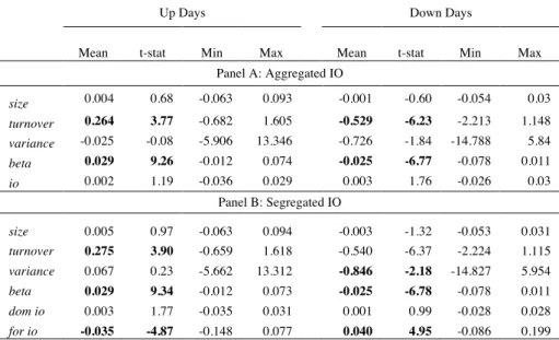
The event-days are defined as (a) up market, days in which the market return is two-standard deviations above its eleven-year average (from 2000 to 2010) and (b) down market, days in which the market return is two standard deviation below its eleven-year average (from 2000 to 2010) minus two standard deviations. The dependent variable is the event-day adjusted market return, defined as being the daily return of firm i on event-day j minus the eleven-year average (2000-2010) of firm’s i return. The independent variables are size, defined as the natural logarithm of the firm’s equity 50 days prior to the event-day; turnover, which is the daily volume of a stock expressed as a percentage of the total number of shares outstanding on the event-day; variance which is the market model residual variance for the period [-250,-50]; beta, computed as the beta of stocks daily returns with the market return for the period [-250, -50]; io, which is the percentage of IO on the capital structure of a company on the event-day. Results are presented for both aggregated and segregated IO, divided into dom io, which is the percentage of domestic IO on the capital structure of a company on the event-day and for io, which is the percentage of foreign IO on the capital structure of a company on the event-day. The table presents the mean, minimum and maximum coefficient estimated. It is also reported the t-statistic corresponding to a test of the mean being different from zero.

Up Days Down Days

Mean t-stat Min Max Mean t-stat Min Max Panel A: Aggregated IO size 0.004 0.68 -0.063 0.093 -0.001 -0.60 -0.054 0.03 turnover 0.264 3.77 -0.682 1.605 -0.529 -6.23 -2.213 1.148 variance -0.025 -0.08 -5.906 13.346 -0.726 -1.84 -14.788 5.84 beta 0.029 9.26 -0.012 0.074 -0.025 -6.77 -0.078 0.011 io 0.002 1.19 -0.036 0.029 0.003 1.76 -0.026 0.03 Panel B: Segregated IO size 0.005 0.97 -0.063 0.094 -0.003 -1.32 -0.053 0.031 turnover 0.275 3.90 -0.659 1.618 -0.540 -6.37 -2.224 1.115 variance 0.067 0.23 -5.662 13.312 -0.846 -2.18 -14.827 5.954 beta 0.029 9.34 -0.012 0.073 -0.025 -6.78 -0.078 0.011 dom io 0.003 1.77 -0.035 0.031 0.001 0.99 -0.028 0.028 for io -0.035 -4.87 -0.148 0.077 0.040 4.95 -0.086 0.199

The liquidity factor is also important for institutions. Institutional investors choose stocks with a high level of liquidity since they usually have large positions on their capital structure and need to be able to trade. This is only possible with stocks that can be traded in high volumes. Agarwal (2007) examines the relationship between IO and liquidity, finding results similar to Falkenstein (1996) and Lesmond, Ogden and Triznka (1999), that conclude that

(17)

institutions prefer more liquid stocks due to safety or reduced transactions costs by trading in big blocks. Not surprisingly, our results show that turnover is very related to the market adjusted returns, being the second variable with more statistical significance for both up and down market event-days. During the event-days, higher turnover is associated with larger market swings, (positive for the up market event-days and negative for the down market event-days). These results suggest that firms that are more liquid, experience large market movements.

Kothare and Laux (1995) and Falkenstein (1996) found evidence that links institutional holdings with more volatile stocks. Their comprehensive data found that institutional investors, compared against individual investors, prefer stocks with high idiosyncratic volatility. Falkenstein (1996) specifically, using data covering the period of 1991 and 1992, finds that mutual funds have a preference for high-volatility stocks. On the other hand, Sias (1996) has empirical evidence that fits this previous findings, but goes against the interpretation that institutional investors choose to select riskier stocks. In fact, he shows that an increase of IO on stock’s capital structures may be the reason of increase on volatility. Nevertheless, it is not the goal of this analysis to try to understand what is the cause of the volatility, but only to avoid bias on our results, therefore the variable variance is included on the abnormal return regression. Another reason to include this variable on the regression, is attribute to Dierkens (1991) that proposes that idiosyncratic volatility is a useful measure of informational asymmetry. Since institutions are informed market agents, this implies a negative relationship between the level of informational asymmetry and the level of IO. The variance results are inconclusive. For the up market event-days, it is not found any relationship between the adjusted market returns and stock’s variance, while for the down market event-days there is some statistical significance between the two variables. Since beta is also a proxy of a stock’s risk, it is imperative to include it on the regression. Omitting this variable could also bias our results. The largest statistical significance that is found, concerns the stock’s beta. As it was expected, firms with higher betas, have on up market event-days larger returns, while for down market event-days present smaller returns.

The variable of main interest for the analysis is the IO. The goal is to try to find statistical significance, once this would suggest that institutional investors react to large market swings. IO only is important for the down market event-days and only at the 10% significance level. The coefficient of 0.003 also suggests that there is small economical significance. While the

(18)

level of IO is not so significant for aggregate levels, when split into domestic and foreign IO, the results are surprisingly different. Panel B shows that the level of foreign IO during days of extreme returns is significantly related with the levels of stock’s abnormal returns, for both types of event-days. Despite the high level of significance, the coefficient magnitude shows that stocks with higher levels of IO have smaller absolute returns on the event-day. In fact, the results from our regression lead us to conclude that foreign institutions are not contributing to the extreme returns verified on the event-days, contradicting the general trend in the market on such days. On the other hand, the results for domestic institutions on such event-days do not lead to any conclusive result. The level of significance of the domestic IO variable is low and it is not in line with institutional herding during these extreme days. It is important to notice that even if there is some relationship between the two variables, it is not possible to be sure that the large market swings are caused by institutions and not by individuals’ decision. These institutions, as banks and mutual funds, are vehicles used by individual investors to trade. The decision to buy or sell is not only dependent of the money managers. Individuals can also be the cause for institutions to sell or buy during these event-days since they give the order to trade. Overall the empirical results for the abnormal return regression suggest that on event-days, foreign institutional herding is much more visible than domestic one. The level of significance of aggregate IO is low for both types of event-days, however when compared with DS empirical findings, it is important to highlight a small improvement. For the up market event-days, DS obtained a t-statistic value of 0.46 with a coefficient of 0.001 while for the down market event-days, the t-statistic and coefficient value remain low, being -0.82 and -0.001 respectively. On the other hand, DS also presents results for IO decomposed. Their findings conclude that different types of IO have different behaves on such event-days, suggesting that specially managers from mutual funds, pension funds and endowments herd and trade with the momentum.

The reason to use the equal-weighted data is connected with the possible bias that could happen. With the value-weighted data, the methodology could pick days in which larger firms had moved more than smaller ones. As it was previously said, size is highly correlated with the level of IO of a firm. Conditioning our analysis to the value-weighted data could have biased our results. Overall the results obtained are not so satisfactory in terms of our prediction. The cross-sectional distribution of returns on the event-days can be related to the level of IO of the firms, but only has statistical significance for the down market event-days.

(19)

3. Abnormal Turnover Evidence

The previous results showed that there is a relationship between the event-day abnormal return and the level of IO, and stronger for foreign IO. A possible cause for the relationship between abnormal return and IO can be the trade volume. If during these market extreme days, institutions buy (up market event-days) or panic and sell (down market event-days), a high level of volume shall be noticed. This section aims to understand the relationship between turnover and institutional ownership.

On Table I, the descriptive statistics have shown that firms with higher level of IO, are more liquid firms. However, as it was stated before, literature findings say that institutions prefer more liquid stocks. In order to take further conclusions about the relationship between turnover and firm’s level of IO, it is necessary to compare it against abnormal turnover. A comparison between regular turnover and low or high levels of IO would not bring any valid conclusions. Abnormal turnover is defined as the difference between the daily turnover of firm i on event-day j and the eleven-year average (2000-2010) of firm’s i turnover (unconditional average). Stocks that compose the high IO subsample have on average higher values than the low IO portfolio (corresponding to a mean of 0.0004 for the low IO portfolio and a mean of 0.0024 for the high IO portfolio for the up market event-days and a mean of 0.0003 for the low IO portfolio and a mean of 0.0017 for the high IO portfolio for the down market event-days). The t-test to determine if the means of the two subsamples are equal, rejects the equality at one percent significance level.

The purpose of this regression is to try to understand if the variable IO has any statistical significance relatively to the abnormal turnover. If the level of firms’ IO is associated to the abnormal turnover, one can infer that in fact, on such event-days, institutions are contributing to the increase of liquidity and therefore they can be herding and trading with momentum. Fama and MacBeth (1973) regressions are used:

!"#$%_! =γ_!+γ_!!"#$_! +γ_!!"!"#$%&_!+γ_!!"_!+ !_! (2)

where the dependent variable, aturn, is the event-day abnormal turnover, the difference between daily turnover of firm i on event-day j and the eleven-year average (2000-2010) of firm’s i turnover. Turnover is defined as the daily volume of a stock expressed as a percentage of the total number of shares outstanding on the event-day. Since firms with higher levels of IO have on normal days higher values of turnover, it is necessary to compute

(20)

a control variable to make sure that these firms maintain the high levels of turnover on days with extreme returns. The abnormal turnover, previously defined, shall be a good measure. The independent variables are size, variance and IO. The decision to include size and variance as control variables are related to the preference of institutions to larger firms and higher levels of idiosyncratic risk, as explained in the previous section.

On Table IV, the results are presented for up and down event-days and are divided into Panel A which aggregates IO and Panel B which disaggregates IO into domestic and foreign.

Table IV

Event-Day Abnormal Turnover Regression – All stocks

This table presents the estimates of the event-day abnormal turnover regression on IO and control variables for the market:

!"#$%!= !!+ !!!"#$!+ !!!"#$"%&'!+ !!!"!+ !!

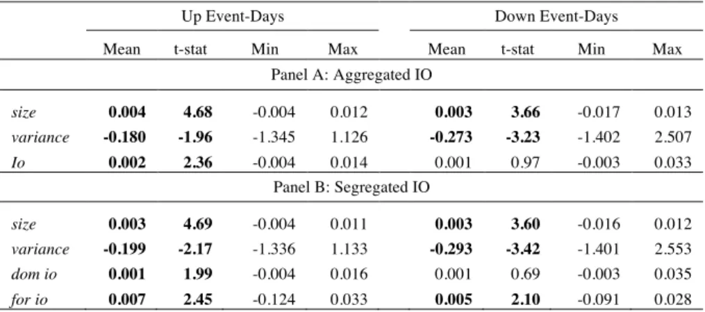
The event-days are defined as (a) up market, days in which the market return is two standard deviation above its eleven-year average (from 2000 to 2010) and (b) down market, days in which the market return is two standard deviation below its eleven-year average (from 2000 to 2010). The dependent variable is the event-day abnormal turnover, the difference between daily turnover of firm i on event-day j and the eleven-year average (2000-2010) of firm’s i turnover. The independent variables are size, the natural logarithm of the firm’s equity 50 days prior to the event-day; variance, the market model residual variance for the period [-250,-50]; io, the percentage of IO on the capital structure of a company on the event-day. The table presents the mean, t-statistic for a null hypothesis of zero mean, minimum and maximum coefficient estimated.

Up Event-Days Down Event-Days Mean t-stat Min Max Mean t-stat Min Max

Panel A: Aggregated IO size 0.004 4.68 -0.004 0.012 0.003 3.66 -0.017 0.013 variance -0.180 -1.96 -1.345 1.126 -0.273 -3.23 -1.402 2.507 Io 0.002 2.36 -0.004 0.014 0.001 0.97 -0.003 0.033 Panel B: Segregated IO size 0.003 4.69 -0.004 0.011 0.003 3.60 -0.016 0.012 variance -0.199 -2.17 -1.336 1.133 -0.293 -3.42 -1.401 2.553 dom io 0.001 1.99 -0.004 0.016 0.001 0.69 -0.003 0.035 for io 0.007 2.45 -0.124 0.033 0.005 2.10 -0.091 0.028

First, size matters. On such extreme days, there is a considerable statistical significance between the firm size and its abnormal turnover. Its average coefficient of 0.004 and 0.003 also shows that besides its statistical meaning, size also has an economical significance. The results for the second control variable of the regression also show that variance is contributing to the level of abnormal turnover of the firms, more on the down market event-days than on the extreme positive days. The IO coefficient is positive and highly significant for the up market event-days, supporting the idea that on days that there is a huge increase on the

(21)

market, institutions herd and trade with the momentum. On the other hand, the results for the down market event-days do not sustain the herding behaviour on such extreme days (t-statistic 0.97). Despite these inconclusive results, when IO is disaggregated, the variable of foreign IO turns out to be statistically significant, suggesting that firms with higher levels of foreign IO have larger abnormal turnovers on the event-days. Again, fitting the previous results from the abnormal return regression, there is some evidence that foreign institutions react to large market swings. Comparing the results with those of Dennis and Strickland (2002), the conclusions are in clear contrast. Their empirical results regarding the abnormal turnover and IO, identify a relationship between the two variables during both types of event-days, leading them to conclude that during the extreme event-days, institutions are the cause for the abnormal turnover. The two control variables have no statistical significance. Their evidence suggests, more than ours, that institutions herd together and trade with the momentum of the market.

The regression results concerning the aggregate IO are very different for the two types of event-days and overall it is not possible to suggest that the cause for the abnormal turnover on such event-days come from institutional trades. However, it is possible to infer that in fact, foreign institutions seem to have a relationship with both abnormal returns and abnormal turnovers on days with large market swings. Another possible inference that can be made, is that firms with more market capitalization are the ones that are contributing more to such abnormal turnover levels.

4. Post-event Performance

The empirical findings regarding the event-days variables have not been so conclusive about the contribution of institutions to the extreme returns verified on such days. However, for the up (down) market days, the high IO firms have event-day returns higher (lower) than the low IO firms. This statistical evidence fits the idea that institutions herd on such days and contribute to such extreme returns. However, this would not be a problem if in fact institutions were driving stock’s prices to their fundamental value.

Table V presents six months returns after the event-days to ascertain if institutions are (a) contributing to market efficiency or (b) if they are just trading with the momentum contributing only to market volatility. If six months after the event-day stock’s prices go back to their previous values, institutions just contributed to market volatility and contrarian

(22)

strategies can be used to take advantage of this mispricing. Table V presents results for all firms and for several cuts. First, we divide the sample into non-IO firms and IO firms. Then we sort IO firms into quintiles based on IO on the event-day. Panel A and B present the results for up and down market event-days, respectively. The first row presents the average of the percentage of IO on the event-days for each of the subsamples. The second row presents the event-day return average. The third row presents the average of the six months returns (125 days) after the event-day. The post-event return averages are tested to see if they are significantly different from zero. The standard deviation, skewness and kurtosis are computed next. The last row contains the average number of stocks on the event-days. To avoid a bias, all returns and averages are equal-weighted, since institutions own on average larger firms (Gompers and Metrick (2001); Bennett, Sias and Starks (2003); Campbell, Ramadorai and Schwartz (2009)).

Up and down market days have different contrasting results. The average of event-day return for the up market event-event-days is similar to all the subsamples, except for the first quintile IO firms. From this, it is not possible to conclude that institutions trade more than individual investors on those same event-days. However, using post-event 125-return, IO firms have significant positive returns whereas non-IO firms have negative returns. The difference between the two type of firms is statistically significant. These conclusions are in clear contrast to our expectations if institutions would herd, i.e., if in fact institutions herd during the event-day and move the stock’s price away from their true value, then a negative six month post-event return, moving the stock’s price to its prior value.

On the other hand, the results from Panel B (down market event-days) lead us to think that in fact on such extreme days, institutions have herd and deviate stock’s prices from their true value. Although, the event-day return average is not sufficient to conclude that IO firms have more negative returns than non-IO firms on the event-days, the difference between the post-event performance of low IO firms and high IO firms is sufficient to infer a different behaviour between institutions and individuals. IO firms six month post-event returns are statistically positive and different from the non-IO firms. This shows that the market correct the previously oversell by institutions on the event-day and moved the stock’s prices back again to their previous value.

This is in line with Schnusenberg and Madura (2001). After examining six US indexes, they report underreaction to extreme positive event-days and significant reversals over a 60

(23)

day period following negative market shocks. This results are consist with the Uncertain Information Hypothesis (UIH), a hypothesis put forward by Brown, Harlow and Tinic (1988) that states that after the release of new information regarding a security creates considerable uncertainty. Therefore an investment on that security entails additional risk for the investor

Table V

Post-event Performance Statistics – All stocks

This table presents the post-event performance statistics for all stocks. The sample is divided into non-IO firms and IO firms. IO firms are sliced into quintiles on IO. The first row contains the average of IO on the event-day. The event-days are defined as (a) up market, days in which the market return is two standard deviations above its eleven-year unconditional average (from 2000 to 2010) and (b) down market, days in which the market return is two standard deviations below its eleven-year unconditional average (from 2000 to 2010). The event-day return is the average of the event-day returns. The post-event return is defined as being the 6-month return (125 days) after the event-day. It is also computed a post-event return average for each of the eleven subsamples. This table presents an average of the standard deviation, skewness, and kurtosis on the event-days. The average number of stocks in portfolio is an equal-weighted average of the number of stocks that each of the subsamples contains on event-days. Subsample’s post-event return averages are tested to check if they are significantly different from zero. Non-IO firms IO firms IO firms – Non-IO Low IO firms Q2 Q3 Q4 High IO firms High IO – Low IO High IO – Non-IO All firms

(I) (II) (II) – (I) (1) (2) (3) (4) (5) (5)-(1) (5)-(I)

Panel A: Up Event-Days Instit. ownership (%) 0.00 62.72 62.72 18.10 46.15 68.52 84.06 96.75 78.65 96.75 61.69 Event-day return (%) 4.05 4.24 0.19 2.96 4.23 4.67 4.71 4.66 1.69 0.60 4.24 Post-event return (%) -1.84 9.58 11.41 8.86 10.42 9.97 9.71 8.93 0.07 10.77 9.39 t-statistic -0.52 2.93 12.34 2.90 3.04 2.97 2.85 2.77 0.07 9.77 2.87 St. deviation 0.27 0.25 0.07 0.24 0.27 0.26 0.26 0.25 0.08 0.09 0.25 Skewness -0.77 -0.82 0.24 -0.73 -0.68 -0.52 -0.94 -1.25 -0.44 0.37 -0.81 Kurtosis 1.29 1.80 -0.50 0.93 1.38 1.29 2.10 3.05 0.01 -0.46 1.77 Average # stocks 38 2,409 482 482 482 482 482 2,447

Instit. ownership (%) 0.00 63.53 63.53 18.66 47.15 69.55 84.98 97.31 78.65 97.31 62.64 Event-day return (%) -4.67 -4.53 0.14 -3.52 -4.61 -4.88 -4.94 -4.71 -1.20 -0.04 -4.54 Post-event return (%) -6.67 6.37 13.03 4.07 6.76 7.22 6.91 6.89 2.83 13.56 6.19 t-statistic -1.71 1.85 13.39 1.30 1.88 2.08 1.89 1.97 3.07 11.84 1.79 St. deviation 0.32 0.28 0.08 0.26 0.30 0.29 0.30 0.29 0.08 0.09 0.28 Skewness -0.84 -1.03 -0.08 -0.88 -0.88 -0.77 -1.18 -1.37 -0.88 0.18 -1.03 Kurtosis 0.90 1.36 -0.56 0.87 1.01 1.00 1.64 2.12 0.49 -0.40 1.34 Average # stocks 34 2,476 495 495 495 495 496 2,509

and a rational investor will require an additional premium as compensation for the additional risk. The main consequence of this theory implies that after a very negative event-day, average abnormal returns will be positive and post-positive event abnormal returns will be non-negative, in case investors show decreasing absolute risk aversion. Lasfer, Melnik and

(24)

Thomas (2003) use a similar methodology and also report findings consistent with the UIH, i.e. investors overreact to bad news and as a consequence observe significant reversals but underreact to good news and observe significant positive post-event returns.

Regarding the up market event-days results, it is also possible to link with ideas first introduced by Bikhchandani et al. (1992) and Welch (1992), the informational cascades. The basic concept of this type of herding, is that agents see what other agents have previously done and prefer to ignore their own private information. For example if an agent has information that may convince him not to buy a certain stock, but he/she sees that other institutions have bought it, the agent prefer to ignore its private information and go along with the herd. As Keynes (1936) thought, the stock market is like a beauty contest where judges choose the winner not because she is the most beautiful but because they think that other judges will pick her. Overall what our results for the up market event-days can show is some evidence of bubbles, caused by herding, namely informational cascades. Again, if institutions are herding and contributing only for the growth of a bubble, at a certain point, the market shall correct stock’s prices and move it again to its fundamental value.

The findings on this paper are similar to those of DS. The different behaviour of institutions on both types of event-days is also verified on their post-event statistics which fits to our previously justifications fitting the UIH.

5. Conditional Event-Day Definition

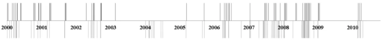
This section tests the same hypothesis that institutional ownership is linked to extreme stock return movements using a rolling window definition of event-days. We use the same methodology as before but an event-day is defined when the market return is two standard deviations above its one-year moving average, up market day, or two standard deviations below its one-year moving average, down market day. Between 2000 and 2010 there were 71 up market event-days, with an average return of 3.39% and 109 down market event-days with an average return of -3.36%. On Figure 2, the distribution of events over time is presented. It is clear that most events cluster over time. In comparison to the unconditional definition of event-days, most of the events are the same, but now our sample increases mostly in the period before 2007.

(25)

Figure 3. Conditional event-days. Above the timeline are registered the up market event-days and below the timeline are registered the down market event-days.

We estimate Equation (1) to understand the relationship between IO and abnormal return on these event-days. The level of significance for the aggregated IO variable for both types of extreme days increased. The t-statistics of 1.35 and 2.28 for the up market event-days and for the down market event-days respectively, show that for our out-of-sample test, the relation is more significant than before. The results for the segregated IO are completely different. The variable of foreign IO lacks statistical significance and the relation between the domestic IO variable and the abnormal returns continued to be statistically insignificant.

The biggest improvement registered is linked to estimation model (2), concerning the relation between the abnormal turnover and the level of IO on the event-days. For both types of event-days, the variable of aggregated IO registers very high t-statistics, suggesting a relation between the two variables. Regarding the segregated IO, the foreign IO variable loses its statistical significance but on the other hand, the domestic IO variable suffer an improvement regarding its significance. With t-statistics of 6.45 and 4.81 for the up and down market event-days respectively, we can conclude that during the event-days, firms with higher levels of domestic IO are contributing to the abnormal levels of turnover.

Evidence from the post-event performance, suggest that during the event-days, firms are in fact herding. When the event-day returns is decomposed into the 5 quintiles, it is possible to conclude that stocks with higher levels of IO are the ones that have the most extreme returns, for both types of event-days. The similarity with the analysis that was done on Section III.4. ends it here. The post-event performances results are inconclusive. In fact, stocks that do not have any IO are the ones that six months after the event-day have the most extreme returns.

IV. Extreme Stocks

In this section, we focus only on the stocks that (a) on the up market event-days had returns two standard deviations above its unconditional average and (b) on the down market event-days had returns two standard deviations below its unconditional average. We expect institutional herding to be more visible when we exclude the stocks that do not contribute for the general trend of the market on that day.

(26)

1. Event-Days Descriptive Statistics

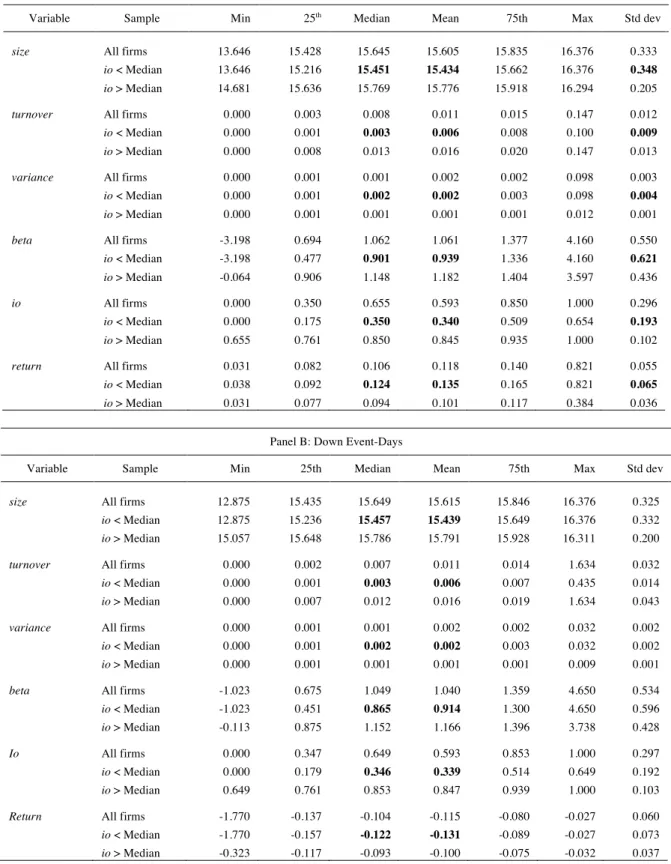
Table VI presents the descriptive statistics for the event-days for stocks with extreme returns as stated before and its structure is the same as Table II. The size statistics again, show that institutions prefer stocks with bigger size. An average size of 15.605 and 15.615 for up and down market event-days, corresponds to an increase of size on our stock’s sample when compared with Section III. The increase is not statistically significant but since institutions prefer stocks with a bigger size, our sample of stocks with extreme returns show signs of being a sample with more IO, which lead us to think that institutions in fact can be contributing more for the extreme returns. In terms of liquidity, the turnover variable in comparison with the previous analysis, show signs of increase. Our sample now is composed by stocks with higher levels of turnover than before. Again it lead us to think that our sample has higher levels of IO since institutions prefer more liquid stocks. When decomposing the turnover variable into the two subsamples, again it is possible to confirm that stocks with higher levels of IO are much more liquid than the others. The variance statistics do not show any significant change however it confirms that institutions prefer stocks with low levels of idiosyncratic risk when compared with others. The beta statistics show that our sample for this Section IV has stocks with more systematic risk. Again, when beta statistics are decomposed, it is possible to confirm that stocks with a higher level of IO prefer stocks with bigger betas. Taking into account that previous literature and our statistics show that institutions prefer these kind of stocks, it lead us to think that our sample of stocks with extreme returns have in fact higher levels of IO which can be a sign of their contribution to extreme returns on the event-days. When analysing the IO statistics, it is possible to confirm that there is an increase of the presence of institutions on our stock sample. An average of 59.3 percent represents an increase of 0.9 and 0.3 percent of the level of IO on the up and down market event-days respectively. An increase of the level of IO on this sample, would lead us to think that in fact institutions could be contributing more to the extreme returns but in fact, the return statistics lead us to think that this may not be happening. Despite the increase on absolute values of the returns for both types of event-days (more positive returns for the up market event-days and more negative returns for the down market event-days), the descriptive statistics show that in fact higher returns on up market event-days are associated with stocks with low levels of IO and lower returns on down market event-days are associated

(27)

Table VI

Event-Day Descriptive Statistics – Extreme Stock Returns

This table presents the descriptive statistics for the 60 up market event-days (Panel A) and for the 68 down market event-days (Panel B). This table is structured as Table II.

Panel A: Up Event-Days

Variable Sample Min 25th _Median _Mean _75th _Max _{Std dev}

size All firms 13.646 15.428 15.645 15.605 15.835 16.376 0.333

io < Median 13.646 15.216 15.451 15.434 15.662 16.376 0.348

io > Median 14.681 15.636 15.769 15.776 15.918 16.294 0.205

io < Median 0.000 0.001 0.003 0.006 0.008 0.100 0.009

io > Median 0.000 0.008 0.013 0.016 0.020 0.147 0.013

io < Median 0.000 0.001 0.002 0.002 0.003 0.098 0.004

io > Median 0.000 0.001 0.001 0.001 0.001 0.012 0.001

beta All firms -3.198 0.694 1.062 1.061 1.377 4.160 0.550

io < Median -3.198 0.477 0.901 0.939 1.336 4.160 0.621

io > Median -0.064 0.906 1.148 1.182 1.404 3.597 0.436

io All firms 0.000 0.350 0.655 0.593 0.850 1.000 0.296

io < Median 0.000 0.175 0.350 0.340 0.509 0.654 0.193

io > Median 0.655 0.761 0.850 0.845 0.935 1.000 0.102

return All firms 0.031 0.082 0.106 0.118 0.140 0.821 0.055 io < Median 0.038 0.092 0.124 0.135 0.165 0.821 0.065

io > Median 0.031 0.077 0.094 0.101 0.117 0.384 0.036

Variable Sample Min 25th Median Mean 75th Max Std dev

size All firms 12.875 15.435 15.649 15.615 15.846 16.376 0.325

io < Median 12.875 15.236 15.457 15.439 15.649 16.376 0.332

io > Median 15.057 15.648 15.786 15.791 15.928 16.311 0.200

io < Median 0.000 0.001 0.003 0.006 0.007 0.435 0.014

io > Median 0.000 0.007 0.012 0.016 0.019 1.634 0.043

io < Median 0.000 0.001 0.002 0.002 0.003 0.032 0.002

io > Median 0.000 0.001 0.001 0.001 0.001 0.009 0.001

beta All firms -1.023 0.675 1.049 1.040 1.359 4.650 0.534

io < Median -1.023 0.451 0.865 0.914 1.300 4.650 0.596

io > Median -0.113 0.875 1.152 1.166 1.396 3.738 0.428

Io All firms 0.000 0.347 0.649 0.593 0.853 1.000 0.297

io < Median 0.000 0.179 0.346 0.339 0.514 0.649 0.192

io > Median 0.649 0.761 0.853 0.847 0.939 1.000 0.103

Return All firms -1.770 -0.137 -0.104 -0.115 -0.080 -0.027 0.060 io < Median -1.770 -0.157 -0.122 -0.131 -0.089 -0.027 0.073 io > Median -0.323 -0.117 -0.093 -0.100 -0.075 -0.032 0.037

(28)

with stock with low levels of IO. Beside this, the subsample of stocks with high levels of IO has a standard deviation much smaller. This statistics show signs of institutional herding in a different way that was expected. What is shown is that institutions are not contributing to the extreme returns, in fact they are contributing to contradict the general trend in the market on such days.

2. Abnormal Return Evidence

The independent variables used to compute the regression are the ones analyzed on the previous section. Like before, the technique used to compute the regression is the Fama and MacBeth (1973) one. We use the previously defined estimation model (1).

The dependent variable ari is the market adjusted return for firm i on the event-day j. The market adjusted return is defined as being the difference between the eleven-year unconditional average (2000-2010) of stock’s i return and stock’s i return on the event-day j. The coefficients used to make our conclusions are the time-series average of the coefficients of the several event-days. Table VII presents all the results for the abnormal return regression. The results are divided into Panel A, aggregated IO and Panel B, disaggregated IO.

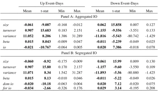
Table VII

Event-day Adjusted market Return Regression – Extreme Stock Returns

This table presents the result for the event-day adjusted market return regression on IO and control variables for the equal-weighted market following model (1) for extreme stock returns. This table is structured as Table III.

Up Event-Days Down Event-Days

Mean t-stat Min Max Mean t-stat Min Max Panel A: Aggregated IO size -0.061 -9.087 -0.168 -0.012 0.062 15.858 0.007 0.127 turnover 0.907 15.683 0.183 2.151 -1.155 -9.556 -3.551 0.133 variance 11.052 8.206 1.386 31.289 -11.816 -5.543 -80.742 -1.429 beta 0.015 8.043 -0.009 0.047 -0.011 -5.239 -0.049 0.025 io -0.021 -10.767 -0.064 0.005 0.020 7.386 -0.018 0.078 Panel B: Segregated IO size -0.060 -8.92 -0.175 -0.009 0.061 15.99 0.009 0.130 turnover 0.907 15.80 0.170 2.137 -1.157 -9.60 -3.550 0.109 variance 11.071 8.34 1.542 31.287 -11.893 -5.56 -80.880 -1.425 beta 0.015 8.13 -0.010 0.046 -0.011 -5.22 -0.049 0.026 dom io -0.020 -10.18 -0.063 0.004 0.020 7.12 -0.020 0.075 for io -0.034 -2.66 -0.326 0.176 0.029 3.14 -0.195 0.208

(29)

statistical significance for both types of event-days, a very different result from the previous analysis. However, the empirical results from the regression show that the relationship between size and abnormal return is slightly different from what would be expected. Although the size of a firm is related with its abnormal return on the event-day, size is not contributing to an increase of the absolute return on such days, in fact bigger firms have smaller absolute returns on extreme days, which is possible to confer by the value of the coefficient (-0.061 for up market event-days and 0.062 for down market event-days).

On the other hand, the relation between turnover and abnormal return is as it was expected. With a t-statistic of 15.683 and -9.556 for up and down market event-days respectively, the level of abnormal returns is intrinsically related with the level of liquidity of the stocks, being an increase of turnover a sign of increase of the absolute abnormal return of a stock for both types of event-days. The main variable of interest for our analysis, IO level, lead us to different conclusions for each of the event-days. For the up market event-days, the average coefficient for IO is -0.021 with a t-statistic of -10.767. There are no questions that on up market event-days, there is a relation between the abnormal returns and the level of IO of a firm, leading us to think that in fact institutions can herd on such days. However, institutions herd in a different way that it was expected. They are not contributing for the extreme returns verified in such days, in fact they are herding on the opposite direction. Despite the herding evidence during the up market event-days, it is not possible to say that institutions are buying and contributing for the extreme positive returns. The segregation of IO by types of institutions as DS do on their work, would show if this is the general trend for all types of institutions or if there are any outliers. On their empirical results, DS show that different institutions react differently to these event-days. Institutions as banks and insurance companies do not contribute for the abnormal returns on such extreme-days, in fact they react as our results also show, on the opposite direction. Regarding the results of the IO variable for the down market event-days, the high level of statistical significance and the value of the coefficient fit the same idea. On such days, institutions herd but on the opposite direction. Overall, the empirical results show evidence of herding but in fact institutions are not contributing to the extreme returns verified on such days. The coefficients values show that in fact institutions are herding on the opposite direction and that this kind of investors are not the ones contributing for the extreme returns on such days. The different results that are registered on our analysis can be due to different reasons but the main difference from DS sample is the