Pricing of Reverse Mortgages : an application exercise to the portuguese market : does it make sense?

(1)

Pricing of Reverse Mortgages: An application exercise to the Portuguese market Does it make sense?

Marco Paulo Pedro Barata

Advisor: Professor Joaquim Cadete

Dissertation submitted in partial fulfilment of requirements for the degree of Master in Finance, at the Universidade Católica Portuguesa

(2)

ii CATÓLICA-LISBON

School of Business & Economics

Pricing of Reverse Mortgages: An application exercise to the Portuguese market Does it make sense?

Marco Paulo Pedro Barata July 2017

Abstract

Pricing Reverse Mortgages (RM) is particularly challenging for loan providers, especially due to the uncertainty related with termination timing and the volatility of economic variables such as interest rates and house prices. When a no negative equity guarantee is offered, as Reverse Mortgages do, these variables are the ones that most significantly impact the size of the losses and the timing on termination for the lenders. This Master Thesis studies the risks that a lenders faces when providing this type of loan and the pricing of RMs applied to the Portuguese case, by estimating the house price and the required reverse mortgage interest rate when considering a RM annuity and a RM lump sum.

Keywords: Reverse Mortgage, VAR Model, VECM, pension, Semi-Markov multiple state model, No Negative Equity Guarantee, Portugal

(3)

iii

Acknowledgments

Foremost, I would like to express my sincere gratitude to my friends and former colleagues Maria for her motivation and Rita for the continuous support and for her patience.

I am grateful to D. Esmeralda for being there whenever she was asked to without saying “no” or “let me check”.

I would like to thank my parents Celeste and José, for all the support they gave me throughout my life.

Last but not the least, to my son Vasco and my wife Susana, for being the light of my life and the reason for never giving up fighting to be better every day.

(4)

iv

5. Conclusion ... 40 Appendices ... 42 Appendix I ... 42 Appendix II ... 43 Appendix III ... 44 Appendix IV ... 45 Appendix V ... 46 Appendix VI ... 47 Appendix VII ... 48 Appendix VIII ... 49 Appendix IX ... 50 Appendix X ... 52 Appendix XI ... 53 Appendix XII ... 54 Appendix XIII ... 56 References ... 58

(6)

vi

List of Figures

Figure 1 – Age dependency ratio, young (% of working-age population) ... 42

Figure 2 – Age dependency ratio, old (% of working-age population) ... 42

Figure 3 - Mortgage, Equity and House Value Simulation (bankwest a Division of the Commonwealth Bank of Australia). ... 43

Figure 4 -Mortgage loan vs Reverse Mortgage loan balances. ... 43

Figure 5 - ACF and PACF analysis ... 45

Figure 6 - Normality test for the Variables. ... 48

Figure 7 - Impulse response from shock in RLnHPI ... 50

Figure 8 - Impulse response from shock in RLnHPI ... 50

Figure 9 - Impulse response from shock in LnLC ... 51

Figure 10 - Impulse response from shock in LnGDP ... 51

Figure 11 - Swap rate curve obtained from the spot rates for the AAA- Euro Area Government bonds ... 53

Figure 12 - Female mortality at age 65. ... 53

Figure 13 - Female survival rate at age 65 ... 53

Figure 14 - House price simulations (base 100 for 1st quarter 2009) ... 53

Figure 15 - Three-dimensional plot of the expected VaR 95% for different applicable RM interest rates and annuity payments (65 years old borrower is assumed ... 54

Figure 16 - Risk vs VaR 95% chart for an annuity RM ... 55

Figure 17 - Changes in VaR 95% and VaR 99% from changes in house price estimated evolution (annuity) ... 55

Figure 18 - Changes in VaR 95% and VaR 99% from changes in borrower's age at contract start (annuity) ... 55

Figure 19 - Three-dimensional plot of the expected VaR 95% for different applicable RM Interest Rates and LTV (65 years old borrower is assumed) ... 56

Figure 20 - Risk vs VaR 95% chart for lump sum RM ... 57

Figure 21 - Changes in VaR 95% and VaR 99% from changes in house price estimated evolution (lump sum) ... 57

Figure 22 - Changes in VaR 95% and VaR 99% from changes in borrower's age at contract start (lump sum) ... 57

(7)

vii

List of Tables

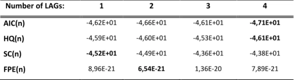
Table 1 – VARselect from R – selection methods ... 28

Table 2 – VARselect from R – Values calculated for each Method ... 28

Table 3 – Johansen Procedure (Test type: trace statistic without linear trend and constant in cointegration). ... 29

Table 4 – Loan Parameters ... 34

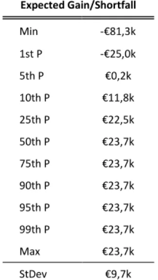
Table 5 - Expected payoff/shortfall for the annuity base case scenario ... 36

Table 6 - Expected VaR 95% for different applicable RM Interest Rates and annuity payment (65 years old borrower is assumed) ... 37

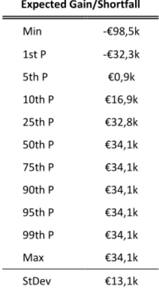
Table 7 - Expected payoff/shortfall for the lump sum base case scenario ... 38

Table 8 - Expected VaR 95% for different applicable RM Interest Rates and LTV (65 years old borrower is assumed)... 39

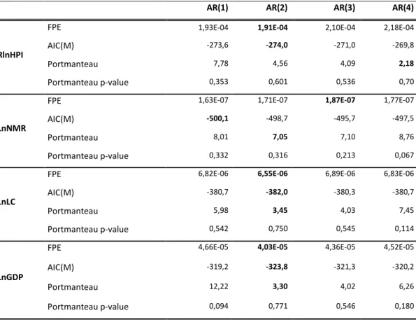
Table 9 – Autoregressive order determination ... 46

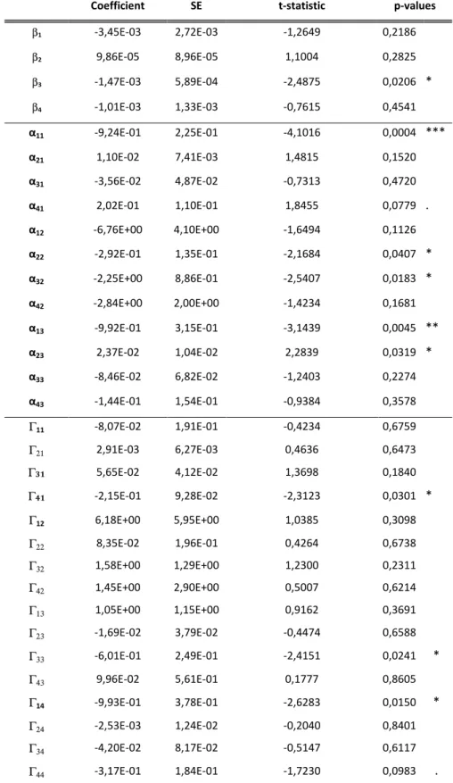
Table 10 – Significance tests for VECM coefficients ... 47

Table 11 – Residuals Correlation Matrix ... 49

Table 12 – Residuals Correlation p-values Matrix ... 49

Table 13 – Residuals Correlation Matrix (New) ... 49

Table 14 – Residuals Correlation p-values Matrix(New) ... 49

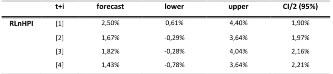
Table 15 – One year forecast of the VAR Model ... 49

Table 16 – Forecast Error Variance Decomposition ... 52

Table 17 - RM interest rates for a RM annuity (2% upfront insurance premium and 1% annual fee) ... 54

Table 18 - Expected median for different applicable RM Interest Rates and annuity payments (65 years old borrower is assumed) ... 54

Table 19 – RM interest rates for a Lump Sum RM (2% upfront insurance premium and 1% annual fee) ... 56

Table 20 – Expected median for different applicable RM Interest Rates and LTV (65 years old borrower is assumed)... 56

(8)

1

1. Introduction

Reverse Mortgages can be resumed as a mortgage loan offered to older borrowers, that give their home as collateral, without having to move out or without the need of repayment until the contract termination which, most probably would occur at the time of death of the borrower. Generally, with the age the health care expenditure by the elderly people increases substantially. For the retirees the pension, itself is often too short and additional sources of income, such as the Reverse Mortgage, would clearly be a plus. Reverse Mortgages is still an unexplored universe in Portugal. Two questions may be asked: 1) Does it make sense to offer this type of products in Portugal? 2) What is missing in the Portuguese market?

During this master thesis we will address those two questions regarding the Reverse Mortgages by analyzing the Portuguese current and required conditions to develop the Reverse Mortgage market, address existing regulatory issues and analyze the advantages and disadvantages of the product to both Borrowers and Lenders. We will be focusing on the pricing of reverse mortgages for the Portuguese market by estimating the house prices and the Interest rates, some of the macroeconomic variables with the most significant impact on the timing and Size of the losses for the Issuer.

This paper is divided in 4 sections. In the first section we present a Literature Overview on reverse mortgages, the concepts, features and risks. We will also dedicate a topic to the RM around the World and the Portuguese current environment. On the second section we will focus on the reverse mortgage pricing, from the pricing of the RM variables to the final model for RM. The third section of this work is dedicated to an actual case, where we will address our model through the simulation of the variables applying the Monte Carlo simulations method. Finally, we will present the conclusions taken from the study and the next steps regarding this subject.

(9)

2

2. Literature Overview (Concepts, Features and Risks)

During the last century, the World has faced a considerable number of crises. The impact of those crises is normally measured (or attempted to be measured) in terms of an immediate result (e.g. unemployment rate increase, budget deficit impact) or, at the best, at a medium term (e.g. the impact of new legislation created). The impact of some of those crises, such a Demographic change, may however, prevail for a much longer period of time and have a significant impact many years later.

A good example is the end of the World War II, when many countries around the World and particularly in Europe observed a demographic birth boom also known as the Baby Boom.1 Considering 2016 as a reference, the baby boomers should be today between 52 and 70 years old, meaning most of them are reaching, or will reach soon, the retirement age. Also important to refer is the life expectancy rate which is currently near its peak (LeDuc Media, 2015). As one may imagine, the scenario we now face constitutes on its own, a major challenge for Private and Public Pension Systems, particularly for those with a Defined Benefit Pension plan, where an unfunded or Pay-as-you-go2_{financing model was put in place.}

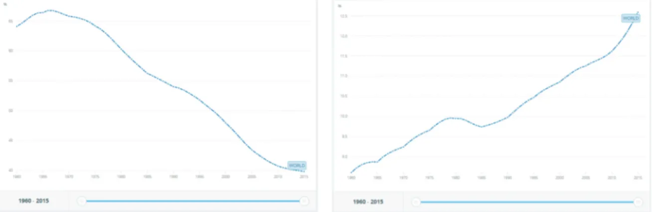
Well, the real challenge is even bigger. During the last 2 decades, several financial crises took place, starting with the Japanese Real Estate Crisis, followed by the Technological Bubble, the Subprime crisis and, more recently, the Sovereign Debt Crisis. All of these crises were responsible for creating a significant uncertainty environment that led to an observed reduction of the birth rates all over Europe3. This new generation of babies now have between 0 and 20 years (using again 2016 as the ending date) meaning they are now starting their professional careers. In turn, the retirees are growing rapidly in number with longer life expectancy, while new entrants on the Labor Market are decreasing significantly. The same conclusion is drawn from the World Bank’s indexes of the Age Dependency Ratio for young and old people (measuring the % of young/old individuals in terms of the working-age population). The Age Dependency ratio (Young), illustrated in Figure 1 from Appendix I, show a steady decrease in global terms reaching in 2015 the lowest figure (39.8%) since 1960.

1

According with the United States Census Bureau the baby boom period took place between mid-1946 and mid-1964

2_{“‘Pay-as-you-go’ is a financing model for the Pension Systems where the workers’ current contributions pay for pensioners’} current benefits. The alternative means of financing retirement incomes is through funding, where workers’ contributions are invested. Accumulated contributions and investment returns then pay for the pension.”´ (The World Bank, 2005)

3_{Data from the Eurostat database show that the births rate in the European Union countries as a whole is near its historical low} rate since 1960 and decreasing in average since the 60’s. (European Comission, 2016)

(10)

3 Regarding this ratio, Portugal ranks 18 between the countries with the lowest ratio (22%) within 241 countries. (The World Bank(1), 2016)

The Age Dependency Ratio (Old), illustrated in Figure 2 from Appendix I, show us the opposite scenario with the index constantly increasing and reaching 12.6% in 2015 its highest point since 1960 in terms of the universe of countries. Portugal ranks 6th in this list with 31.9%. (The World Bank(2), 2016)

As previously mentioned, the challenges for the Pension Systems are huge. For a Defined Benefit Pension System to be financially sustainable, the actuarial value of the assets must be in equilibrium with the future responsibilities of the system. The way to reach this equilibrium will always depend on the financing model that is adopted, either Pay-as-you-go or funded, resulting in different types of measures or dimension of these measures that should take place in case the equilibrium is lost4. The profitability of a system based on the funding model will depend on the interest rates evolution while a Pay-as-you-go system will depend on the rate of increase of the population (Carneiro, 2013).

In Portugal, like in many other European countries, the Social Security System and most of the Private Pension Systems are based on the Pay-as-you-go Model, where the current assets and contributions fund the current responsibilities, supported in the expectation that the future contributions will be enough to cover future responsibilities. The recent change in demographics along with the high level of unemployment (not yet referred) has led to the Portuguese Pension System loss of the Equilibrium, in which the income is far from fulfilling the expenses.

The Size of the Annual Pension Responsibilities in terms of the Portuguese National Budget correspond to nearly 20%, and has, for the last few years, increased in absolute terms, from around €21 billion in 2010 to around €24 billion in 20145_.

In order to fill the gaps, transfers from the Public National Budget have been increasing in many OECD countries. Some extraordinary transfers have also taken place. In Portugal, an extraordinary tax (CES – Extraordinary Solidary Contribution) was created, and was paid by retirees from 2011 until the end of 2016.

However, to restore the equilibrium of the system, more deep measures are required, albeit some might have significant political impact and entail loss of political popularity.

4_{The Debate on the most adequate means of finance the Pension Plans is extensive all over the globe, particularly related with} the contribution in terms of slice of the national annual budget. See (Carneiro, 2013) for the Portuguese case.

(11)

4 “Raising state pensionable age, or perhaps more specifically linking it explicitly to

expected longevity, is generally a key policy in ‘parametric’ reforms to the problem of financing public pension programmes. A number of OECD countries are changing pension ages” (Disney, 1999).

With the change introduced with the Decree Law 83-A/2013 of 30 December (Assembleia da República, 2013), the retirement age in Portugal increased from 65 to a variable age as defined by Ministerial order each year. The resulting retirement Age will be 65 plus the number of months necessary to reflect a sustainability adjustment associated to the increase of life expectancy above 65 years old. In 2017, the Retirement Age was fixed at 66 years and 3 months and for 2018 it was increased 1 month to 66 years and 4 months. (Assembleia da República(1), 2017)

The increase of restrictions for early retirements was also noteworthy, with an impact on the retirement conditions for those with ages below 60. Previously, early retirement ages were allowed at 55, without significant impact on the retiree’s income. (Assembleia da República(2), 2016).

As such, for the retirees, or prospective retirees, the retirement conditions suffered a significant deterioration over the last years and consequently, in their life conditions, particularly for those retirees with a high dependency on the pension plan’s income.

It is important for retirees to find alternative ways to complement and fund their pensions, and reduce their dependencies from government’s pension support.

Reverse Mortgage Contracts (RM), although with no significant expression in Portugal6, play an important role as a complement to individual pensions in countries like the UK, Australia and the United States of America.

Usually, RM are non-recourse loans where the borrowers (generally people above 65 years old) agree to receive either a lifetime rent, a lump-sum amount, a line of credit or a mix of the previous alternatives, giving their home as guarantee for the loan while at the same time keeping the right (and obligation) to live in their home until the termination event occurs. The Termination event defines the moment at which the loan becomes payable to the provider of the loan. It occurs when the homeowner dies, leaves or sells the house. The amount of the loan will only be paid after the termination event occurs through the proceeds from the sale of

6_{At the beginning of 2017 Banco BNI Europa started to provide Reverse Mortgages contracts to senior borrowers with 65 year old} or more (https://www.publico.pt/2017/04/19/economia/noticia/bni-lanca-credito-cereja-para-clientes-com-mais-de-65-anos-e-com-casas-para-hipotecar-1769220 )

(12)

5 the home. In other words, if the homeowner never leaves the house he will never pay for the loan.

In countries like Australia, the inclusion of a Non Negative Equity Guarantee (NNEG) is mandatory7. The NNEG assures that the borrower’s responsibilities will be limited by the value of the home given as guarantee for the loan, with the lender bearing all the losses from the loan in excess of the mortgaged home sale. For the lender, the sale of a RM is similar to writing a put option on the mortgaged home, while the final value of the loan (at termination) is the Strike, and the Exercise Price the Value of the Sale (Ji, 2011).

The final payoff for the contract will depend on the interest rate of the loan, the House Price at termination and the Termination Timing. The existence of these three variables and the significantly different results they can produce makes the pricing of Reverse Mortgages the biggest challenge for the providers of the loan, particularly if their intent is to provide a competitive pricing for the product.

Figure 3 from Appendix II illustrates the different evolutions on value for the Mortgage Loan, the Equity owned by the borrower and the House Prices over time8_{in Australia. The} presentation of these scenarios by the providers of the Reverse Mortgages is included on the Reverse Mortgage Information Statement and is a requirement from the Australian Government under the National Consumer Credit Protection Act 2009. In this example, with the House Price being the only variable and only 11% of the house value being provided to the borrower, we can see that after 20 years the value of the mortgage becomes almost 2/3 of the House Value if no change occurs in the House Value and only 1/3 of the House Value if an increase of 3% on the house price is observed.

The estimation of accurate figures for the evolution of variables like house prices and longevity is a key element for providers of the loan, particularly when there is a NNEG involved.

7_{The Consumer Credit Legislation Amendment (Enhancement) Act 2012 (The Paliament of Australia, 2012) included the Section} 86 subdivision 86B defining “Discharge of debtor’s obligations under credit contract and discharge of mortgage” applicable to the number 1 (a) as defined on the subdivision 86A “the debtor’s accrued liability (whether or not due and payable) under the contract

is more than the amount (the adjusted market value) worked out under subsection (2) for the reverse mortgaged property.”

8

Two scenarios are presented, the first one with a flat house value and the second one a 3% annual growth on the house value. In both cases, the initial house value is AUD450.000 and a lump sum of AUD50.000 and an 8.5% fixed rate is assumed. After 20 years the debt will increase to AUD272.060 and the remaining equity will be AUD177.940 on the first scenario and AUD540.690 on the second scenario. The house price will remain in the first scenario and will grow to AUD812.750 on the second scenario.

(13)

6 2.1. Theoretical Concept of RM

A RM loan is a type of Equity Release Scheme (ERS)9, generally non-recourse loans that allow for senior homeowners, who accumulate a significant part of their savings in the form of assets such as home equity (illiquid assets), while having little in cash, to convert it into cash, mainly for consumption purpose as a complement of their private pensions schemes (Bingzhen, Yinglu, & Peng, 2013).

In a RM contract the homeowners borrow money giving their home as collateral for the loan. During the life of the contract the house must remain as the first address of the borrower, or else a Termination event will be triggered and the loan must be repaid. The Termination event is triggered in the moment the borrower permanently moves out of the house, sells it or dies. In this type of contract the borrower is not required to make any regular payment of principal or interest while borrowers remain living on the mortgaged home. The repayment to the bank will be done by the proceeds from the sale of the house when the borrower dies or leaves home. Due to the existence of a NNEG, the amount of money owed by the borrowers, or their heirs in the case of the death of the borrower, is capped by the sale value of the mortgaged home.

2.1.1. Main Features

The best way to look at a RM is by opposition to a typical (well known) Mortgage Contract. As the name suggests, the main features in a RM act in the opposite direction of a normal "usual" Mortgage Contract.

2.1.1.1. The Loan Amount and Repayments:

The way the loan amount is received by the borrower and the way repayments are done are the first main differences when compared to a typical mortgage. When buying a house with the support of a lenders credit, the borrower receives a lump sum amount and agrees to repay this amount plus some contractual interest (based on a fixed or floating rate) agreed by making periodic payments for a predetermined number of periods (generally between 30 to 50 years on a monthly basis). On each payment, the principal of the loan will be repaid at an increasing rate (Figure 4 from Appendix II) until the Principal in debt becomes zero at the

9

ERS consists of transforming fixed assets in owner occupied dwellings into liquid assets for private pensions (Reifner et al.,

2009(1)). They can take the form of Loan Model ERS or Reverse Mortgages, eventually repaid by from the sale proceeds of the property; or Sale Model ERS or Home Reversions, where the contract starts with the sale of the Home (idem).

(14)

7 maturity of the contract (which was defined when the contract was made). The risk of not recovering the loan amount by the Lender will also decrease with time.

In turn, in a RM, the borrower agrees to receive the loan amount as a lifetime rent, in a lump sum, as a line of credit or as a combination of the line of credit with any of the other two plans10_{. As mentioned above, the repayment of the loan and interest will only be made when} the borrower moves out permanently, sells the house or dies (the termination events). The duration of the contract is unknown until the termination event occurs. The loan amount and interest amount will be increasing at an increasing rate with the passage of time. For the lender, the risk of not recovering the loan amount will also increase with time.

As stated previously, the RM contracts usually have a NNEG clause, which covers for the amount of loan owed that exceeds the sale value of the mortgaged home. Henceforth, the NNEG guarantees that the financial responsibilities of the borrowers or their heirs are not higher than the value of the home.

2.1.1.2. Homeownership:

In a RM, the borrower not only lives in his home but is also the owner of the property. Together with this ownership comes the responsibility for paying all the property taxes, all the repairs required on the property and the existing and required homeowner insurance (American Association of Reverse Mortgage (AARP), 2010).

2.1.1.3. Life expectancy and the Target Audience:

One additional key element when defining the loan amount (not referred above) is the life expectancy. The life expectancy acts in opposite direction when compared with a traditional Mortgage Loan to a RM contract.

In a Mortgage contract, the borrowers are generally younger and healthier, single or couples (between 25 and 35 years old) with significant lifetime expectancy and the expectation of making the regular payments without any incident. The younger the borrower, the higher the loan amount available when comparing similar mortgage contracts. In a RM contract, the relation is the opposite: the younger the borrower the lower the loan amount available. Generally, the RM contracts are available for borrowers above 62 years old. The older the

10_{As reported by the US Department of Housing and Urban Development the line of credit is the most common choice at the US} accounting alone for 68% and in junction with a rent or lump sum contract for an additional 205 of all the RM Contracts at the US (Nakajima & Telyukova, 2014).

(15)

8 borrower the higher the loan amount he will be able to receive in terms of a percentage over the house value as the duration of the contract is expected to be lower.

2.1.1.4. Insurance Premium:

With the uncertainty from the variables previously mentioned and a NNEG in place, the RM Contracts have, from a lenders perspective, a significant level of risk. As Szymanoski refers in his paper (Szymanoski, 1990), if the loan was offered to the market without any type of insurance, it would have to be priced with a substantial premium to cover the risk involved. To minimize the premium, the product should be placed with strict limits on the amount of cash and/or the lender should diversify the investment.

In the US, the insurance is provided by the US Federal Housing Administration (FHA) under the Home Equity Conversion Mortgage (HECM) RM program. By pooling the investments, with both high volume and regional diversification, the risks are reduced enabling lenders to access insurance at a significant lower premium than it would be normally possible.

In general terms, the Premium is, in several countries, set at 2% upfront plus an annual premium as a percentage of the loan outstanding (generally up to 1.25%).

2.1.1.5. Other costs:

Other costs may apply when setting up a RM contract. These costs may include setup fees paid to the lender for processing the loan, third party fees to compensate for the required inspections, house evaluation, mortgage taxes credit checks… and also ongoing fees to be paid regularly, usually on a monthly basis, for the account statements produced among other administrative documents, and exit fees for processing the closure of the contract.

2.1.2. Main Risks

2.1.2.1. The Longevity Risk:

In a RM Contract, the loan amount is only known when the contract termination occurs, as it depends on the borrower leaving the house (as an example moving to a long term care facility) sooner or later, or ultimately dying. In other words, the borrower's longevity plays an important role on the loan amount. Consequently, longevity and the mortality rate are crucial in defining the size of losses if it reaches the crossover point, the point in which the loan amount (including interest accrued) surpasses the selling value of the house. There are some studies regarding Longevity Risk management, such as Wang, Valdez & Piggot that used

(16)

9 Generalized Linear Model (GLM) to project future mortality rates (Wang, Valdez, & Piggott, 2007). On their study they proposed the securitization of longevity risk in RM by the usage of survivor bonds and survivor swaps to hedge the risk within the Reverse Mortgage products and particularly for pricing the NNEG.

We will cover the NNEG pricing in this master thesis by proxy when computing the applicable interest rate for the annuity and lump sum payments of the Reverse Mortgage.

2.1.2.2. Interest Rate and House Prices Risks:

Two other variables are relevant in the Reverse Mortgages pricing computation: the interest rate and the house prices.

If the interest rate applied to the loan is too high (either as a fixed rate or a floating rate with a high spread), the loan will accrue interest rapidly and reach quicker the crossover point than with lower rates.

On the other side of the equation are the house prices and the housing market prices evolution. In a bull market, the crossover point will be far in time, while in a bear market the prices will drop and the crossover point will occur sooner than previously expected. The house prices prediction is a point of major interest in academic papers as it is the basis for all the mortgage market. Nevertheless, until recently only few investigators dedicated time to the modelling of house prices. The Geometric Brownian Motion model is generally accepted for predicting the house market prices as used by Szymanoski (Szymanoski, 1990). Other authors such as (Sherris & Sun, 2010) and (Shao, Hanewald, & Sherris, 2015) Sun & Sherris proposed a Vector Autoregressive (VAR) Model for modelling the house prices based on the most relevant macroeconomic variables. This model will be a central point in our discussion and so we will get back to it soon.

2.2. RM around the World

According to an American Advisors Group article: "The History of the RM" (American Advisors Group, 2014), the first RM contract was designed in 1961 in Portland, US, by Nelson Haynes of Deering Savings & Loan, allowing a widower to continue living in her house after her husband’s death. Since then, the RM Market has grown in the US and from there, to the rest of the World. Nevertheless, the growth we observe is not exaggeratedly high as there is a need, in new countries, to adapt the existing Laws and Legislation to the product specificities.

(17)

10 2.2.1. USA:

In the US, the RM Market is dominated by the existing HECM program which is part of the US Department of Housing and Urban Development (HUD). Under the HECM program, several requirements are set for a RM loan to be accepted. Among others, the borrower can be single or a family living in the mortgaged home, the younger member be at least 62 years old, and they must participate in a consumer information session given by an HUD approved HECM counselor (HUD.GOV, 2016).

As stated in the previous topic, by pooling the investments, the Program provides insurance at a lower cost than Private companies since the Program has the ability to control and limit the market. The major drawback of the HEMC program is the existence of a maximum amount and percentage limits on the loan currently fixed at $625,500 and 100% of the sales price of the property.

Under the HECM program, the borrower can choose between a fixed and a floating interest rate mortgage. When choosing a fixed interest rate, the loan payment will be done as a lump sum. When choosing a floating interest rate, the borrower can choose between 5 payment plans: equal monthly payments to be received for a fixed period of time (Term) or until the last borrower dies or moves out of the residence (Tenure), as a Line of Credit of a pre-determined amount with the Lender or, as a mix between a line of credit and both the tenure (Modified Tenure) or a pre-determined period of time (Modified Term).

2.2.2. Australia:

In Australia, the Reverse Mortgage contracts can be accessed by the age of 55. Not everyone can access to the credit and the amount will vary from lender to lender. As a general rule, the minimum amount is AUD10,000 and the maximum amount (depending on the age) can reach 25 – 30% of the value of the home by the age of 70. The Borrower is protected by the introduction on 18 September 2012 of a non-negative equity guarantee (NNEG), from the Government on all new reverse mortgage contracts, limiting the amount owed to the lender by the market value or sale price of the home. The credit providers are required by law to “lend money responsibly” (Australian Securities & Investment Commission, 2016).

In 2004, SEQUAL, an Association of lenders, aiming to pursue and promote the best practices among the providers of the equity release products and particularly among their members, was established. SEQUAL is highly influential in the Australian Reverse Mortgage market with

(18)

11 an important role on the literacy of Senior Australian Homeowners by raising their awareness on Equity Release Products.

It is also important to refer that the borrowers benefiting from a Reverse Mortgage contract may face some limitations on their rights to receive some types of social assistance and on the pension amount.

The loan can be taken as a lump sum, in a set of periodic payments, as a line of credit or a combination of these 3 options.

2.2.3. EU Member States

In 2009, a Study was conducted for the European Commission with the intent to broaden its knowledge on the existing ERS and developments on each member state.

The study identified 10 Member States with Loan Model ERS. From those, the UK, Spain and Ireland had already developed a significant ERS market (Both Loan Model and Sales Model). France, Hungary, Italy, Finland, Sweden, Germany and Austria were identified as Member States with less developed Loan Model ERS markets. The existence of a developed Mortgage Market is a key element for the development of an ERS market, for this reason, without surprises, UK and Spain appear as two of the European countries with a more developed ERS market. The European market for Reverse Mortgage represented in 2007 less than 0.1% of the overall mortgage market or €3.3bn over €6147bn from around 40.000 contracts (Reifner et al., 2009(1))11.

Regarding the type of Issuers, in Europe Banks represent 42% of the total providers of RM, Real Estate Investors 19%, other Specialist Lenders represent 12%, Insurance Companies 12%, and the remainders 15% are represented by Intermediaries operating on behalf of the previous referred providers.

2.2.3.1. UK

To become eligible for a RM in the UK the borrower needs to have more than 60 years and can establish the RM contract individually or as a couple. The borrowed amount will depend on their age and will be up to a maximum loan-to-value ratio amount set by each provider. The RM Market in the UK, as mentioned, is quite developed. For this reason, the complexity of the products offered is also significant. The loan amount can be released to the borrower in a

11

(Reifner et al., 2009(1)) Identified that Spain and the UK account for around 93% of the all contracts and amount. Nevertheless, in Spain the estimated average amount by contract account for a significant €352k versus €55k in the UK. The total amount is €1,3bn from 3.600 contracts in Spain and €1,8bn from 33.000 contracts in the UK.

(19)

12 lump sum payment, periodic payments, and access to the equity in an ad-hoc basis or, more commonly as a drawdown facility. Many features can be added to the contract limiting the loan amount such as capping the level of indebtedness or guaranteeing the remaining share of the property value.

Unlike the Australian case, there is no NNEG requested by law. Although the Safe Home Income Plans (SHIP), a trade association with 22 members representing over 90% of the ERS market share in the UK, established a Code of Conduct meaning all members offering equity release schemes must abide to by a series of rules which ultimately protect equity release customers. One of such rules, clearly states that it should be given to the borrower a guarantee that he will never owe more than the value of the property under the ERS contract. In respect to the interest rates, they are generally fixed rates for the lifetime of the contract and most of the providers request an additional fee (penalty) in case of early termination. This penalty will decrease as time goes by.

2.2.3.2. Spain

As in the UK, the RM are offered in Spain to homeowners above 60 years old and the borrower can also be an individual or a couple. Although, in the Spanish case, the owner’s residence does not necessarily has to be the mortgaged property. The loan can be released to the borrower in a lump sum amount, in a series of defined number of payments, as a lifetime pension or, most commonly, in the form of a credit line.

The RM Contract consists of a Contract called “Hipoteca Pension” or life pension and is almost always made with a bank acting as an agent to an insurance company.

In 2007, Law 41/2007 introduced significant changes to the Real Estate Credit Market with significant impact in terms of legal aspects related with the Mortgage Market. Also for the RM borrowers and their heirs, some fiscal benefits and protection were introduced. One of these changes was the introduction of the NNEG as a law in the form of a Cap on the amount to be recovered by the provider of the loan, removing from the heirs the responsibility of receiving a heritance of a RM property.

Since 2007, in case of Termination by death of the borrowers, the heirs can: 1) Choose to repay the loan; 2) Take a new credit to keep the property; 3) Leave the home with the provider. The interest rates can be either Fixed or Floating, in the latter, a spread to the reference rate Euribor® is added.

(20)

13 2.3. Reverse Mortgage in Portugal

The ERS market in Portugal has started at the beginning of 2017 and no historic data exists. Some of the other existing products, offered to investors in Portugal, such as the Sale and Leaseback, share some characteristics with the Sale Model ERS, but there are no products that share significant characteristics with the Loan Model ERS or Reverse Mortgage.

The 2009 study on Equity Release Schemes in the EU (Reifner et al., 2009(2)) defined Portugal as a country with no legal framework regarding the ERS market. Nevertheless, the study refers the existing concerns around the legal rights over the mortgaged property and the priority of claims between the lenders and the successors, and the potential legal dispute that could urge from it, as one of the main issues for not offering such a product.

Like the legal framework, there is also no fiscal framework. Without the establishment of benefits or exemptions (e.g. real estate registers), the viability of the Reverse Mortgage market will not be possible, as the costs can potentially be extremely high.

One other aspect to be taken in account is the real estate market conditions and the current social mind-set. Culturally, the Portuguese people buy or build their own home, usually by the time of marriage. The Portuguese Home Ownership rate is significantly high, 74.9% in 2014 when compared with the 69.5% in the European Union or 66.7% in the Euro Area12_. Importantly, real assets account for more than 85% of the Portuguese families’ wealth. If we consider only the property as the primary residence of the Portuguese people it represents 50% of the total wealth (Costa, 2016).

Also important to mention is the current environment lived in Portugal by the potential providers of RM products. Considering that the banks are the main providers of RM in Europe and bearing in mind that bank’s profitability in the last few years has been under pressure severely hindered by high levels of impairments and low levels of interest rates, the inclusion of RM contracts on the portfolio of financial products available for banks customers could represent a new/additional source of revenues.

Finally, banks’ and (also) insurers’ regulatory capital ratios can, not only benefit from higher levels of profitability, but benefit from relatively low risk weight typically associated with collateralized mortgages, vis-à-vis other type of loans. As highlighted in (Thibeault & Wambeke, 2014) residential mortgage loans were not heavily affected with the introduction of

(21)

14 Basel III with the risk weights associated to residential mortgage loans standing at a relatively low level, at 35%13_.

13

The definition of qualifying residential mortgage includes collateral mortgages and reverse mortgages satisfying certain loan-to-value criteria for the Capital Adequacy Ratio assessment and, as so, applies the 35% risk weighted(BIS, 2014).

(22)

15

3. Reverse Mortgage Pricing

Pricing Reverse Mortgages is challenging. As previously said, many variables (e. g. house price, interest rates, longevity, termination rates) and options (e. g. single borrower or couple, lump sum disbursement or periodic payment, among others) need to be considered in the calculations.

As such, different approaches can be followed for the pricing of RM with one common idea: “the present value of the total expected gain equals the present value of the total expected loss” - (Wang, Valdez, & Piggott, 2007) and also expressed by, (Lee, Wang, & Huang, 2012), (Bingzhen, Yinglu, & Peng, 2013) and (Shao, Hanewald, & Sherris, 2015).

For Reverse Mortgage pricing we will consider the proposed model by (Lee, Wang, & Huang, 2012). In their paper the authors consider the special case of reverse annuity mortgages (RAM). Within the RAM model the borrower receives regular annuity payments without making any repayments of principal or interest during the life of the contract. As mentioned by the authors, the model can also be adjusted to other types of RM such as a lump sum disbursement by considering the annuity as zero except for the initial disbursement.

It is also worth noting that when compared to lump sum RM the RAM suffers greater longevity risk since the loan amount will keep increasing, not only by the amount of the Interest but also by the increase of the principal (annuity) and thus, it requires an insurance mechanism (Lee, Wang, & Huang, 2012).

The risk faced by the lender will be addressed by applying a Mortgage Insurance Premium (upfront plus annual premium) so that the equality referred above will have on the left hand the present value of an insurance premium.

In the next chapter of this section we will first present the Reverse Mortgage variables considered for the model and in the end the RAM model.

3.1. The RM Variables

The first step in defining the model is to define the variables. Particularly, we should know what to model, namely the benchmark (if relevant), or the historical data for the variables. As stated previously, the uncertainty around the macroeconomic variables evolution and particularly the house prices and interest rates, lead to higher levels of risk for a Lender in a RM contract. For this reason, an accurate estimation of those variables is a key element for the RM success.

(23)

16 In the following pages we will present the variables, models and methodologies followed for the final objective of pricing Reverse Mortgages.

3.1.1. Housing Price Model 3.1.1.1. The VAR Model

The interest in modelling the house price market is very recent; the Subprime Crisis (more than the bubble itself) was the trigger. Until 2008, the Housing Market was considered a niche and as such, only a residual interest existed in modelling it, and even less in predicting it. The Subprime Crisis and its severe consequences gave focus to the Housing Market and soon, studying, modelling and predicting its movements become an important key point. It was also of major importance to the Eurostat: “The financial and economic crisis has highlighted the importance of correctly measuring the prices of real estate properties.” (Eurostat, 2016). Several papers on the subject have been written since. And some models have been developed or applied to this market. One of this model is the Vector Autoregressive Model (VAR) which will lead us to the projection of the house prices. We will follow here the methodology proposed by Sun & Sherris (Sherris & Sun, 2010) on the VAR for modelling the house prices. The VAR model, was originally suggested in 1980, by the winner of a Nobel Memorial Prize in Economic Sciences, Christopher Sims. The Model/Framework appeared as an innovative alternative to standard econometric models defined by Sims as “one-equation-at-a-time models”14 which were based in “doubtful exclusion restrictions”15. As described in Christiano (2012), and stated in Sims (1980) in a chapter under the same name, the econometric models in use at the time were using “incredible identifications” assumptions. This identification assumptions introduced on the models could state that, in a demand and supply curve, one variable could impact one side of the equation (the supply side, for instance) with no impact on the other side of the equation (the Demand side, for instance).

The VAR Model (or Framework to be more precise) consists in a simultaneous equation system where all the variables are estimated from a combination of lags of its own and also lags of the other variables in the model.16. Let us now define the general specification of a pth-order VAR. A n × 1 vector y is an autoregressive process if and only if:

y = β + β y + ⋯ + β y + ε

14_{(Sims, Macroeconomics and Reality, 1980)}

15_{“Christopher A. Sims and Vector Autoregressions” (Christiano, 2012)} 16

“VAR’s are models of the joint behaviour of a set of time series with restrictions or prior distributions that, at least initially, are

(24)

17 Where ε ∼ i. i. d. Ν 0, σ , i.e. an aleatory process with Ε ε = 0 and Var ε = σ

As stated in Christiano (2010), Sims argued in his paper that the VAR Model would serve three purposes: (1) forecasting economic time series; (2) designing and evaluating economic models; (3) evaluating the consequences of alternative policy actions.

It is important to highlight that Sims considered the Macroeconometric one-variable-at-a-time identification assumptions inappropriate. Assumptions should exist as restrictions to the model but, the impact in both sides of the equation should not be ignored.

Since its inception in 1980s, the VAR model had proved to be of extreme importance for the Macroeconometric practice. Many researchers have dedicated their studies proposing new versions and improvements on the VAR model emphasizing the innovation brought by the Model.

One of the most significant contributes was given by (Engle & Granger, 1987), with the introduction of the concept of cointegration and vector error correction models (VECM), proposing tools for modelling and testing economic relationships over the long run. On their paper, the authors defended that a linear combination of two or more integrated, nonstationary time series, can be stationary or, in other words cointegrated.

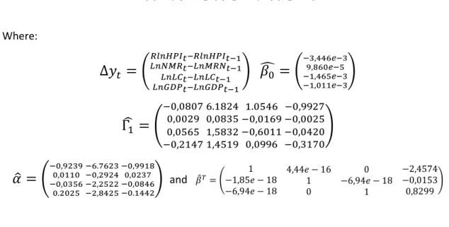
From the VAR(p) process described above we can assess the VECM equation by subtracting the y on both sides and rearranging the terms. The resulting long run VECM will be:

∆y = β + Γ Δy + ⋯ + Γ Δy + αβ y + ε Where:

Γ = − I − β − ⋯ − β , for i = 1, … , p − 1, αβ = Π = − I − β − ⋯ − β

ε ∼ i. i. d. Ν 0, σ , i.e. an aleatory process with Ε ε = 0 and Var ε = σ

Whenever in the presence of Cointegration among the data series, the VECM should be address instead of the VAR model. In practice, after running a VECM, moving from a VECM to a VAR is a straightforward process and most of the software available can manage it easily.

3.1.1.2. The Reference data

For the house prices there is no market reference and only recently a Benchmark was required by the Eurostat, and afterwards developed by the Portuguese Statistic Institute (INE). Until

(25)

18 then, the existing references for house prices were only available from Private Real Estate Companies and speciality sites17_{. In 2014, Evangelista & Teixeira described the development of} the Portuguese House Price Index (HPI) by the INE (Evangelista & Teixeira, 2014). They compared 3 indexes: one composed by the asking prices on a Real Estate site (www.confidencialiobiliario.pt); another one, appraisals-based HPI, based on the bank appraisals data; and the last one, transactions-based HPI, based on administrative fiscal taxes18_.

The HPI currently in use by the Portuguese Statistic Institute is the transactions-based HPI, and it is divided in 4 sub-indexes, discriminating new and existing dwellings and also in apartments or houses. This index incorporated a more complete set of data, as it includes not only the values from transactions (gathered from the IMT), but it also reflects the qualitative changes on the transacted properties19_{(gathered from the IMI).}

The transactions based HPI is a Hedonic Price Index as it takes in account quality differences between dwellings20. Below we present the transaction-based HPI as described by Evangelista and Teixeira (2014).

For all q = (Q-1, Q) and i = 1,…,nq, the HPI approach can be described as follows:

, = + , ; + , + ,

Where,

, , is the price level (or some transformation of it) of the ith dwelling transaction in quarter q; , , stands for the value of the kth characteristic of the ith transacted dwelling in quarter q;

, is a temporal indicator, which is defined as: For all q = (Q-1, Q) and all i=1,…,nq, , = 1, = ,

0, ℎ

, is the parameter associated to the temporal indicator ; and

17_{Imovirtual.pt, on its site give the opportunity to find the house price for each county based on the existing offers for} apartments, dwellings or rooms. Also Confidentialimobiliário.pt presents similar information based on the public Real Estate Site lardocelar.pt.

18_{The HPI as developed by Statistics Portugal is based on the administrative fiscal taxes: the Local Tax on Onerous Transfer of} Property (IMT) and the Local Property Tax (IMI). The index base is 2010 = 100 and appeared as a result from the European Statistics System defined to promote the creation of harmonized official statistics over the European Real Estate Market (Statistics Portugal, 2014).

19

The HPI based on the asking prices represents the first step of the process of selling a property. As so, in a downturn of the market the index will tend to lag the adjustment in price as the asking prices should reflect a higher price than the final transactions. The bank appraisals will only represent the transactions where a bank had intervened as a lender, ignoring the transactions made in cash.

20_{The hedonic methods applied to the house prices are used to take in account the quality differences between dwellings. The} particular characteristics of each house such as number of bedrooms, size, land area, floor level are key elements in determining the price of the properties.

(26)

19

, , corresponds to an error term.

On our study we will be using the transaction-based HPI as the reference data for price of houses to be modelled for RM calculation purpose starting in 2009Q1-onwards.21

3.1.2. Interest Rates 3.1.2.1. The Reference data

In the Reverse Mortgage contracts pricing, the role of the interest rates is extremely important. The loan outstanding balance increase will depend on the level of interest rate (or spread) defined. The interest rates in a RM contract, as stated earlier in this study, can be either a Fixed Rate or a Floating rate. Generally, the fixed rates are higher (from 5% to 8%) and the floating rate is presented as a spread over a perfectly generally accepted rate. For the interest rates in Portugal, Euribor®22_{for 3, 6 and 12 months is widely recognized and used as a} benchmark.

Even though the RM model present in chapter 3.2. applies to both fixed or variable interest rate plus a Spread, we considered in our study a fixed interest rate to determine the outstanding balance increase.

As it will be discussed, the required fixed interest rate to be requested by the lender will be addressed by solving the equation Mortgage insurance premium (MIP) equal to the expected loss for the lender (EL).

To address the Present Value of the future Cash Flows we will consider a Discount factor (B(t)) as suggested by (Lee, Wang, & Huang, 2012) corresponding to the money market account at time t given by:

=

The RM cash flows are, in our study discounted using the Swap rate curve. Since are considering the estimation of long periods (up to 40 years) to access the swap rate curve we

21

Despite the existence of data from Eurostat’s website for periods starting in 2005Q1, we decided not to use it as the data was estimated using methods other than the transaction-based HPI. For the 2005Q1-2007Q4 period was estimated based on non-harmonized data and for 2008 estimated by INE using bank appraisals data (Eurostat, 2016).

22_{“Euribor® is the rate at which Euro interbank term deposits are offered by one prime bank to another prime bank within the}

EMU zone, and is calculated at 11:00 a.m. (CET) for spot value (T+2).” (European Money Markets Institute (EMMI), 2014)

“The choice of banks quoting for Euribor® is based on market criteria. These banks have been selected to ensure that the diversity

(27)

20 will base our calculations on the AAA-rated euro area central government bonds spot rate curve published by the ECB23_.

The data available regarding the referred spot goes from 3 months to 30 years. Bearing in mind we will require the Swap rate curve up to 40 years, additional estimation was executed.

The method followed was the estimation using a time series linear regression of the swap interest rate on the natural logarithm of the time t, the estimation rates considered were the swap rates from year 10 to 30.

3.1.3. Termination Rate

3.1.3.1. The Semi-Markov multiple state model

We have already addressed the impact of interest rate changes and the uncertainty on future value of the mortgage price as key risk factors regarding RM cash flows. The third key element is the termination rate. The termination rate on a Reverse Mortgage will depend on the type of event observed. The most common type of termination is by the death of the borrower(s). This termination type is linked with the higher risk of potential losses for lenders: the longer the life expectancy, the longer the contract and hence the higher the risk. The second reason associated to higher losses to the lender occur when clients move to a retirement home as it usually means that the borrower is already very old and that the outstanding amount could be above the value of the house (the collateral). The third reason is a move for non-health reasons, the borrower will most probably only terminate the loan if there is still some value from the home sale after liquidating the RM. Finally, for refinancing reasons the borrower may decide to terminate the RM contract (Ji, 2011).

The Termination Rate is a key element in defining the timing and size of the gains and losses particularly when having a NNEG in place. There is no defined maturity in such a contract, like in a traditional mortgage contract. Additionally, in opposition to the traditional mortgage contracts, with the passage of time, the amount in debt will increase at an even higher rate and with it, the uncertainty around the final payoff of the RM (gains or losses). If, for the borrower, the repayment is limited by the sale value of the home due to the existence of the NNEG, for the lender, by providing this guarantee, it may represent the assumption of potentially huge losses. For this reason, managing Termination Rates is of major importance for the lender.

(28)

21 While being of key importance, Termination Rates in Reverse Mortgage contracts has been subject to only a couple of studies, as there is also few historical data to support them particularly to model termination, including the reasons other than Mortality. For simplicity, we will address the Termination Rate by proxy to the modelled Joint-Mortality rate for a couple.

In the US, HECM insurance for RM products were initially priced fixing the Termination Rate as being 1.3 times the female mortality rate (Szymanoski, 1990). Years later, in 2007 Szymanoski published a new paper with the data information gathered to date and argued that the original estimation had been conservative.

For modelling for the termination rate we consider the Semi-Markov multiple state model developed by (Ji, Hardy, & Li, 2011) and applied by (Ji, 2011) for the Reverse Mortgages Terminations. The major objective of the original study was to model the dependence between the lifetimes of a husband and a wife. With the application case by (Ji, 2011) the joint-life Mortality was introduced in the Reverse Mortgage context.

Before presenting the model, let μ x, t and , denote, respectively, to the force of mortality for an x-age wife and to the force of mortality for a y-age husband, both in the married status. Let also , , and , , denote, respectively, the force of mortality for an x-age single female and the force of mortality for an y-age single male.

The possible states considered by the semi-Markov joint-life as developed by (Ji, 2011) are three, apart from the State 0 where both the members (wife and husband) are staying at home:

State 1 – Husband is dead State 2 – Wife is dead State 3 – Both are dead

It is important to notice that the move to the State 3 will be the only move corresponding to the termination event.

Given the information above, it is of extreme importance for the Reverse Mortgage pricing to measure the probability of observing a move from any of the States to State 3. In other words, the pricing of Reverse Mortgage depends on the measurement of the probability that the last survivor of a currently wife aged x0 and her husband aged y0 at time t0 will survive at least t

(29)

22 years from now, the same is to mention that a Reverse Mortgage contract signed with the referred couple is not terminated at time t. This probability is denoted as:

= + + : ,

Where,

= − , _{+ + , +}

: = − + + , + + + + , +

One additional remark should be made regarding the Mortality Rate modelling: for simplicity we will assume the borrower’s death as occurring only at the end of each year. For this reason the Mortality Rate will be considered as a proxy for the force of Mortality referred above.

3.1.3.2. The Reference data

Although we present the theoretical model for the Termination Rate, there is no available data in Portugal regarding the Reverse Mortgages in order to simulate the process. Most of the studies we analysed simplified the Termination rate by reducing the estimation to a multiple of the Mortality Rate, generally by multiplying by 1.3 the observed Mortality rate.

Even so, this methodology was considered too conservative for the USA case, since there are significant differences between Portugal and the USA, we will use the same 1.3 multiple of the Female Mortality rate published by the Statistics of Portugal and available in the Peprobe site ( http://www.peprobe.com/pt-pt/document/tabuas-de-mortalidade-para-portugal-2012-2014-ine)

In terms of the model, the adjustment required is straightforward as we will just need to consider the probability of a Reverse Mortgage contract signed with a x-age female not terminated at time t determined by:

(30)

23 As for the Mortality rate no simulation will be done and, despite the positive evolution on the longevity rate, we will assume it as having reached a stable level.

3.1.4. No Negative Equity Guarantee

Though we will not directly address or price the NNEG in this study it will play an important role on accessing the RM annuity payment. From a Lender’s perspective, the NNEG is similar to writing a put option with the Strike being the outstanding balance of the loan in the moment the contract is terminated. In any RM the outstanding balance at the termination moment is unknown and increasing at an increasing step, for this reason pricing the NNEG is challenging. The challenge is even greater if we consider the existence of annuity payments where the uncertainty of the loan outstanding amount will be even greater.

Also important to mention is that the great majority of papers considering some type of pricing for NNEG, such as (Shao, Hanewald, & Sherris, 2015) or (Ji, 2011) considers: 1) only the case were a lump sum exist when settling the contract and 2) the NNEG for the calculation of the so called shortfall (SF) between the NNEG and the Mortgage Insurance Premium (MIP). The MIP will be addressed in the RAM model chapter.

Nevertheless, some important studies and proposals have been done under this subject. In (Wang, Valdez, & Piggott, 2007) the RM risk coverage is treated in terms of the securitization of longevity risk.

The authors present 2 possible solutions: 1) the pricing of Survivor Bonds where the future coupon payments are linked to the proportion of the cohort at issue who remain to be alive at the moment of coupon payment. And 2) the pricing of Survivor Swaps defined by (Down, Blake, Cairns, and Dawson 2006) as “an agreement to exchange cash flows in the future based on the outcome of at least one survivor index”.

3.2. Pricing Reverse Mortgage Contracts

For the pricing of Reverse Mortgages we will consider the payment of a regular annuity (RAM) made to singles or couples without requesting them to make any repayments of principal or interest during the life of the contract.

The RAM was priced using the same approach followed by (Lee, Wang, & Huang, 2012). According to the authors, without arbitrage opportunities, the annuity payment for a RAM can be obtained as the solution for the principle that “the present value of an insurance premium equals the present value of the expected losses from future claims”.

(31)

24 At the maturity of the contract, the borrowers or their heirs are responsible for the repayment of the outstanding balance of the loan ( ) up to the value of the home given as guarantee ( ). At time t, the value of the Reverse Mortgage ( ) which will be the repayment to the lender can be written as the following24:

= , = − − , 0

Where − , 0 is the payoff function for an European put option with Strike price in , which means the non-negative equity guarantee payoff25.

Before assessing the outstanding balance some initial considerations need to be made. The Reverse Mortgage will consider the payment of an upfront insurance premium percentage (π0) on the appraised home equity (H(0)) at contract inception. An annual premium percentage (πm) will also be charged on the outstanding balance. No additional fees or charges will be considered for our study. Although we will assume the mortgage rate as a fixed rate, for the general model we will present the reference interest rate ( plus a spread denoted as πr26. Let x0 and y0 denote the age of the wife and husband27, respectively. At the initial valuation date (t0) we will refer the initial valuation date as 0. We will denote ω as the highest attainable age. The borrower’s death is assumed as occurring only at the end of each year.

The outstanding Balance as described in (Lee, Wang, & Huang, 2012) at the end of year j for j= 1, …, ω - (min(x0, y0)) can be rewritten as:

= ∑ + , , = 1, … . − ,

Where

, = 1 +

0 _{1 +} _, _{= 0}

1 + , = 1, 2, … , − 1

a – represents the annual annuity payment of the Reverse Annuity Mortgage

24_{(Wang, Valdez, & Piggott, 2007)} 25

(Ji, 2011)

26_{For our application case we will simply replace}

+ for a fixed rate r

27_{Based on (Ji, 2011) and (Ji, Hardy, & Li, 2011) some adjustments on the original model were required} in order to consider the couple as borrower and not only single borrowers. Particularly, the age of the borrower at the initial valuation date (t0) will not be x0, as for a single borrower but the minimum between x0 (wife’s age) and y0 (husband’s age).

(32)

25 Finally, under a risk neutral measure Q, we can obtain the present value of the Reverse Annuity Mortgage insurance premium (MIP) by discounting the expected cash flows at each moment considering the probability of survival to the moment 0 by:

= 0 +

,

For the present value of the expected losses (EL) from future claims the same discounting principle must be considered. So that:

= − − , 0

,

The annuity payment (a) should be addressed by solving the equation: = .

(33)

26

4. The RM application Cases

In this section we will dedicate some time to the application of the VAR model to the house prices (in 4.1) and to the parameters estimation (in 4.3) particularly to identify the most adequate RM interest rate (fixed rate) for both the RM annuity and lump sum cases to be used as the base case scenarios on the final analysis. A small chapter dedicated to the Interest rates estimations for the cash flows discount will also be presented (in 4.2).

At the end of this section we will discuss and analyse the results obtained.

4.1. VAR Model for House Prices

The house price estimation is a key element for the pricing of RM contracts. On their paper, Sun & Sherris used data stored for the Australian Market and other data extrapolated from the US Market which was considered to follow the same behaviour. For the Portuguese case this was a challenge. Spain is normally an automatic candidate to be considered similar to Portugal, especially if more data could be used on this study. Unfortunately, the data for the house prices in Portugal and Spain over the last years were far from being similar (Evangelista & Teixeira, 2014), given that Spain experienced a housing bubble market and in Portugal prices were quite stable during the last decade. For this reason, we were only able to consider 32 observations for each of the variables considered.

4.1.1. RM Selection of Variables and proper adjustments

One of the most important steps in any study involving modelling and prediction is the identification of the most relevant variables. This was a real challenge in this study. First, data availability for the HPI in Portugal is recent, only 32 quarterly changes (from 33 observations of the index) could be considered and secondly, the consistency of the used information was of key importance. Information with missing data or with lack of comparability due to changes on the assumptions was excluded (as was the case of the unemployment rate for which a new methodology was introduced in the first quarter 2011. As a result, the unemployment data observed before and after the new methodology implementation are not comparable).

Starting with a total of 8 variables, a detailed analysis of the data was conducted until we got the final 4 variables considered as the most relevant with impact in house prices: