!
Master Thesis
Master of Science in Business Administration Major in Corporate
Finance and Control
Mergers and Acquisitions:
The Case of Delta Airlines and US Airways
Francisco Braamcamp de Mancelos
Supervisor: Peter Tsvetkov
September 2013
Dissertation submitted in partial fulfillment of requirements for the degree of Master in
Business and Administration, at the Universidade Católica Portuguesa, 2013.
Acknowledgments
The conclusion of the present thesis is the culmination of not only six months of particular research on airline mergers and acquisitions, but also the completion of my formal education process.
I have no doubt that this particular paper was the greatest and most challenging academic task I have ever been assigned to, which posed several theoretical and practical difficulties throughout its building process. Yet, considering that along the way I could acquire a set of important skills and understanding related to M&A field, I am certain that based on the final outcome all the difficulties were successfully overcome.
I would like to express my gratitude to supervisor Peter Tsvetkov for his helpful and useful role during the last months, greatly reflected on his availability and valuable feedback.
Last but not least, I am deeply thankful to my family and friends for their tireless support, encouragement and belief in my skills, which were essential to the conclusion of my thesis.
Lisbon, September 2013
Francisco Braamcamp de Mancelos
!
!
!
!
!
!
!
!
!
!
!
!
!
Abstract
Over the last decade, US passenger airline industry faced an extremely adverse period when it comes to profit generation, culminating in significant losses and bankruptcies of several carriers. Within this market, airlines operate under a very demanding and stressful environment. Three main factors are reflective of this specific setting, such as: the existence of unpredictable fuel costs (being the major burden to these firms), the increasing competition forces mainly coming from low-cost carriers and a very economic-sensible air travel demand faced by carriers. Taking into account those industry-specific features, airlines found M&A a strategic tool to increase their profitability by sharing and pooling resources. Ultimately, most recent mega-mergers within this sector are performed aiming at the reduction of capacity in order to strengthen efficiency levels, so the companies can properly weather economic adverse conditions.
In this paper, a proposed merger of equals between Delta Airlines and US Airways is analyzed in order to attest a further step on US airline industry consolidation. Simultaneously, the thesis is expected to fill the blanks about how much value would be yielded by combining these carriers not only from a macro perspective, but also assessing how much value would be captured by each party.
The paper found that the deal would be supported by the generation of cost synergies due to the fact that both companies have a considerable portion of overlapped business operations, specially reflected on identical routes. Indeed, the final results of the report show that after the combination of both firms – including the net effect of synergies -, the value would be 22.6% higher than the enterprise value of the simple combination of each firm based on their standalone valuations. Despite of such positive outcome, this paper took into account the role of antitrust authorities on the process, which can influence the final result of the deal, due to the fact that, after the proposed deal, the combined firm would get a considerable stake of the market, posing questions at the competitive level.
!
!
!
!
!
!
!
Table of Contents
!
1. Introduction 1
2. Literature Review 2
2.1 Valuation Approaches 2
2.1.1 The Components of Discounted Cash Flow Models 3
2.1.2 WACC Model and Adjusted Present Value Method 9
2.1.3 Relative Valuation 11
2.2 M&A Essentials 12
2.2.1 Categories of M&A 12
2.2.2 Methods of payment 13
2.2.3 Synergies 13
2.2.4 M&A and return for shareholders 16
2.2.5 Conclusion 17
3. Company and Industry Analysis 18
3.1 Airline Industry overview 18
3.1.1 Market structure and Market share 20
3.1.2 Costs 22
3.1.3 Revenues 24
3.1.4 M&A trends in airline Industry 25
3.2 Company Analysis 27
3.2.1 US Airways Group 27
3.2.2 Delta Airlines 30
4. Rationale For the Proposed Acquisition 33
5. Stock Performance 34
6. Standalone Valuation 35
6.1 Performance Forecast and Valuation 35
6.1.1 US Airways Group 36
6.1.2 Delta Airlines 52
7. Valuation of The Merged Company 63
7.1 Merged Firm Without Synergies 63
7.2 Merged Firm With Synergies 64
7.2.1 Financial Synergies 65
7.2.2 Operating cost Synergies 66
7.2.3 Capital expenditures 70
7.2.4 Net working Capital 71
7.2.5 Questioning the realization of revenue synergies 71
7.2.6 Integration Challenges and Regulatory reviews 72
7.3 Merged Firm With Synergies 74
7.4 Distribution of Synergy Benefits 75
8. Acquisition 76
8.1 Exchange ratio 77
9. Conclusion 79
10. Appendices 80
List of Figures
Figure 1: Graphical Representation of Beta 7
Figure 2: Unbundled Value of a Firm resorting to APV model 11
Figure 3: The Meet the premium line 15
Figure 4: The Matrix Capabilities/Market Access 15
Figure 5: How the value may be distributed by shareholders between the two parts 17
Figure 6: Domestic Operating Profit and Loss of Major US Major Airlines 18
Figure 7: Per Capita Disposable Income and Revenue Passenger miles 19
Figure 8: Annual US Domestic Average Itinerary Fare 21
Figure 9: Market Share by network and low-cost carrier sub sectors 21
Figure 10: Market share by network and low-Cost carrier sub sectors measured in RPM 22
Figure 11: (a) Cost breakdown for US Airline Industry in 2009; (b) Cost per Available Seat Mile
(CASM) with and without Fuel 23
Figure 12: Leverage of Airline industry expressed by debt-to-investment ratio 23
Figure 13: Total Operating revenue by source 24
Figure 14: Industry RPM and ASM 25
Figure 15: Consolidation of the US Airline Industry from 2000 to 2011, % of domestic
Passenger Capacity 26
Figure 16: US Airways Group Organization Structure 27
Figure 17: (a) Annual revenue by operational segment; (b) Passenger revenue breakdown in
RPM 28
Figure 18: (a) Operational expenses breakdown in 2012; (b) CASM vs. CASM ex. Fuel and
Fuel expenses’ relevance on operating costs 29
Figure 19: (a) US Airways Net Income (loss) from 2008-2012; (b) CASM vs. RASM 2010-2012 29 Figure 20: (a) Annual revenue by operational segment; (b) Load factor in percentage,
passenger revenue per ASM in cents and Passenger yield per mile 31
Figure 21: (a) Operational expenses breakdown in 2012; (b) Operating expenses and CASMs 31
Figure 22: Delta Airlines Net income (loss) between 2009 and 2012 32
Figure 23: 2-year Historical Stock prices: Delta Airlines and US Airways 34
Figure 24: Growth prospects for US Airways revenue segments (2007-2022) 38
Figure 25: (a) Projections for average price per gallon (USD) and Fuel consumption; (b) US
Airways projected aircraft fuel expenses 39
Figure 26: Projections for Aircraft rent expenses 40
Figure 27: Depreciation and Amortization projections 41
Figure 28: US Airways Capex projections 42
Figure 29: Net Working Capital projections 44
Figure 30: Sensitivity analysis adjusting probability of default 50
Figure 31: Equity and enterprise value for different cost of capital 52
Figure 32: Growth prospects for Delta’s revenue segments (2009-2022) 53
Figure 33: (a) Projections for average price per gallon (USD) and Fuel consumption; (b)
Delta’s projected aircraft fuel expenses 54
Figure 34: Capex and D&A projections for Delta Airlines 56
Figure 35: Net Working capital projections for the forecasted period 57
Figure 36: Sensitivity analysis adjusting probability of default 61
Figure 37: Equity and enterprise value for different cost of capital 63
Figure 39: Aircraft fleet of individual firms and combined firm as of 2012 70
Figure 40: Index of quarterly average domestic airfares 72
Figure 41: Distribution and sources of synergies in millions 76
List of Tables
!
Table 1: FAA Classification of airline segments 20
Table 2: Relative financial performance analysis of US Airways and Delta Airlines 32
Table 3: Historical stock information for Delta Airlines and US Airways 35
Table 4: Actual Annual % growth of household disposable income per capita and average
annual % growth rate forecast per regions (2013-2022) 37
Table 5: Current Assets and Current Liabilities as percentage of revenues 43
Table 6: Historical effective income taxes for US Airways 44
Table 7: 2012 Debt ratios for comparable firms at market value 45
Table 8: US Airways Valuation inputs 47
Table 9: Valuation Output using WACC 48
Table 10: Peer group multiples 51
Table 11: Sensitivity Analysis 51
Table 12: Historical effective income taxes for US Airways in million dollars 55
Table 13: Current Assets and liabilities items as a percentage of revenues 56
Table 14: Delta valuation inputs 59
Table 15: Valuation Output using WACC 59
Table 16: Peer Group Multiples 61
Table 17: Delta Valuation sensitivity analysis 62
Table 18: Merged Firm enterprise value without synergies based on WACC model 64
Table 19: Merged Firm enterprise value without synergies based on APV model 64
Table 20: Combined Firm WACC inputs 66
Table 21: Combined firm with financial synergies 66
Table 22: Operating cost synergies after the merger 69
Table 23: Capex potential savings 71
Table 24: Valuation of the Combined firm considering synergies 75
Table 25: Historical Exchange ratio between US Airways and Delta Airlines stock 77
Table 26: Exchange ratio and ownership control 78
!
List of Appendices
Appendix 1: US Nominal GDP projections 80
Appendix 2: Inflation projections for the US 80
Appendix 3: World GDP projections 81
Appendix 4: Passenger enplanements from 2000-2011 81
Appendix 5: Domestic and International Passenger Traffic in RPMs 82
Appendix 6: Accumulated losses and gains within the US Airline Industry per segment 82
Appendix 7: Industry Load Factor from 2000-2012 82
Appendix 8: Historical prices for jet fuel per gallon 83
Appendix 10: Average fare based on domestic itineraries 84
Appendix 11: Recent merger deals within the US Airline Industry 84
Appendix 12: S&P rating and default spread by credit rating 84
Appendix 13: Combined firm's area of influence within the US market 85
Appendix 14: US Airways Income Statement for 2007-2022 86
Appendix 15: US Airways aircraft fuel expenses projections based on FAA forecasts 86
Appendix 16: US Airways Net Working Capital for 2007-2022 87
Appendix 17: US Airways Fleet Composition as of 2012 87
Appendix 18: US Airways Free Cash Flows and Valuation based on WACC 88
Appendix 19: Unlevered Value of the company 88
Appendix 20: Interest Tax Shields 89
Appendix 21: Financial Distress costs and APV outcome 89
Appendix 22: Delta Airlines Income Statement from 2007-2022 90
Appendix 23: Delta Airlines Aircraft fuel expenses based on FAA forecasts 91
Appendix 24: Delta Airlines Net Working Capital 2007-2022 91
Appendix 25: Delta Airlines Fleet Composition as of 2012 92
Appendix 26: Delta Airlines Free Cash Flows and Valuation based on WACC 92
Appendix 27:Unlevered Value of the company 93
Appendix 28: Interest Tax Shields 93
Appendix 29: Financial Distress Costs and APV outcome 93
Appendix 30: Combined Firm with no synergies. 94
Appendix 31: Financial synergies incorporated in FCFFs 94
Appendix 32: Operating costs synergies incorporated in FCFFs 95
Appendix 33: Capex synergies incorporated in FCFFs 95
Appendix 34: Combined firm gross Enterprise Value 96
List of Abbreviations
!! Probability of default
APV Adjusted Present Value
ASM Available site mile
!! Beta levered
!! Beta unlevered
CAGR Compound annual growth rate
CAPEX Capital Expenditures
CAPM Capital Asset Pricing model
CASM Costs per available seat mile
CFD Cost of financial distress
D Debt
D&A Depreciation and amortization
DOJ Department of Justice
DOT Department of Transport
E Equity
EBIT Earnings before interests and taxes
EBITDA Earnings before interests, taxes, depreciation and amortization
EV Enterprise value
FAA Federal Aviation Association
FCFF Free Cash Flow to Firm
g Growth rate
GAO US Government Accountability Office
HR Human Resources
IATA International Air Transport Association
K Cost of capital
LCC Low-cost carrier
M&A Mergers and acquisitions
MOE Merger of equals
MTP Meet the premium line
MV Market Value
NOL Net Operating Losses
NPV Net present value
NWC Net Working Capital
P/E Price-to-earnings
PBGC Pension Benefit Guaranty Corporation
PP&E Property, Plant and Equipment
PV Present Value
PV (its) Present value of interest tax shields
RASM Revenue per available seat mile
!! Cost of Debt
!! Cost of Equity
!! Risk free rate
!! Market return
R&D Research and Development
S&P Standard and Poor’s
SEC Securities and Exchange Commission
SIC Standard Industrial Classification
SVAR Shareholder value at risk
!! Corporate tax rate
Vu Unlevered Value
WACC Weighted average cost of capital
WC Working capital
!
1. Introduction
The present paper approaches the case of a proposed merger between two American airlines, namely Delta Airlines and US Airways. Both carriers turn out to have considerable portions of the American market and are considered to be amongst the US top air carriers in terms of revenues. The aim of the thesis is to assess the sources of potential value creation and how such deal should be structured. Logically, those two final points are the result of a thorough research on finance theoretical concepts applied to the reality of US airline industry, which was intensively studied.
Taking into account that the assessment of hypothetical synergies is associated with some levels of subjectivity and uncertainty, this paper is strongly supported by a theoretical framework exposed in literature review. This section provides widely accepted principles by academics and practitioners with respect to company valuation and all associated concepts one should be prudent when handling them. Moreover, literature review will also cover important facts within M&A topic, portraying the in-between steps companies usually follow when pursuing the conclusion of such deals as well as the most recent trends within this field.
The next section, Industry and Company Analysis, will provide a valuable overview of the US airline industry, based on the depiction of how this market is organized; which market players one should take into account and how this industry has performed over the most recent years. Simultaneously, both companies will be presented through the representation of their revenue, cost, operational and financial past performance, which will provide a reliable and clear picture of their situation, this being crucial to perform the forecasting of several variables.
Company Valuation section shows a detailed process of forecasting the most important drivers that will influence decisive inputs for both companies’ standalone valuation. For each company, three valuation methods were used (discounted cash flow based on WACC method, adjusted present value model and relative valuation), in order to add robustness to the findings.
The last section of the paper analyses the potential value creation when combining Delta and US Airways, through the assessment of the sources of synergies as well as their respective valuation. Lastly, the acquisition itself is going to be analyzed presenting its most important details. Simultaneously, the paper will propose the fair terms that should be implied in this deal in order to enable the agreement between these two firms to go forward.
2. Literature Review
Mergers and acquisition has been a topic of great interest: it has been deeply studied by academics and also widely used by practitioners and managers as a strategic tool. Indeed, until 2007 M&A activity was soaring by reaching in that year more than 4.000 deals involving roughly $4.5 trillion worldwide.
Such popularity among world business is the ultimate reflection of a belief from managers that the combination of two entities generates an extra value – commonly referred to as synergies – that would not be attained if those companies operated on an individual basis (Damodaran, 2005).
Yet, M&A outcome with regard to synergies generation is inconclusive and, consequently, has created two schools of thought across academics. While some average statistics show that most acquisitions do not create value for acquiring shareholders and are often based on whims and “attraction to control and power” (Eccles et al. 1999), Bruner (2005) refuses the average outcome of those statistics arguing that each merger is case-specific and its success may be linked to particular features of the industry, economy, market structure and companies involved. Throughout academics, the following analysis found no precise evidence of the certainty of success or failure of M&A in the majority of industries.
The following section of this analysis will provide insight into the most common approaches regarding company valuation - that will serve as the theoretical base for this analysis’ conclusions – as well as a thorough review of some fundamentals aspects of M&A
topic based on past academic research
.!
2.1 Valuation Approaches
Valuation is surely one of the most important and widely used tools in the world of finance. Its relevance for financial specialists and academics has always been central, though, nowadays it has also been increasingly important for general managers as they become more assertive in resource-allocation decisions (Luehrman, 1997a).
For the sake of consistency, the literature review will only cover the valuation models that are either relevant for the application of the thesis topic or those which are widely accepted by academics and practitioners.
By pointing out these requirements, two valuation models arise: The DCF technique – entailing different perspectives of how a cash flow should be discounted – and the Multiples technique – which presents various ratios. The major difference between these methodologies lies, as Damodaran (2006a) simply clarifies, on a philosophical disparity: while DCF methodologies focus on the intrinsic value of an asset driven by the value created along the future and discounted to the present at a certain rate entailing a given amount of risk, the multiples method finds an asset value by assessing what the market has offered for an asset with similar characteristics.
Furthermore, academics have also researched about what could be the most legitimate and reliable method to be used. DCF models were considered as the most reliable valuation methodology (Kaplan & Ruback, 1996), and have been regarded as the most widely practice for valuing assets, projects, divisions and companies (Koller et al.,2010). However, the level of reliability of a valuation methodology is intrinsically linked to the level of accuracy of the assumptions and forecasts. Thus, multiples analysis can be a strong provider of reliability to forecasts and DCF valuations by sourcing comparability of those in
order to assess if one’s company valuation is higher or lower than what the market has been offering (Koller et al., 2010).
2.1.1 The Components of Discounted Cash Flow Models
DCF methodology is based on the cumulative sum of all the forecasted expected cash flows the firm will generate which will be discounted at the opportunity cost (the return the company would earn in a similar risk level project composed by the value of time as well as a the risk premium),(Luehrman, 1997a).
Hereafter, a thorough analysis will be made to each one of the elements that compose any DCF method: starting with the components of Free Cash Flow to Firm (FCFF), the components of the cost of capital and, finally, some insight about the clash between some of the far and wide used models: DCF using weighted average cost of capital (WACC) and the Adjusted Present Value (APV).
!"#$%"&%'!!"#$% = ! !"#$%&$'!!"#ℎ!!"#$! (1 + !)! !
!!!
Free Cash Flow to Firm
In order to value the firm as a whole - including equity – one should use the Free Cash Flow to Firm, which entails the residual cash flows after meeting operational expenses and taxes, but before debt payments (Damodaran, 2006a):
!"!! = !"#$%!!"#!!"#$%&'()!!"#$%& − !"#$% − !"#$"%&'(&)* − ∆!"
This cash flow is widely used in DCF based on WACC models as well as on the APV model, as it will be demonstrated later.
Throughout the following analysis, the term WACC approach refers to the model, which resorts to FCFF as cash flows used, being discounted at the weighted average cost of capital. Despite some unanimity among practitioners and academics that considered WACC approach as the primary model to be used in valuation over the last quarter of 21st century, new models have come to challenge its dominance (Luehrman, 1997a), such as the APV as later it will be covered.
!"#$%!!"!!ℎ!!!"#$ = !"!!! (1 + !"##)! !!! !!! + !"!!!. (1 + !) !"## − ! (1 + !"##)!
Growth
Growth is an extremely crucial input for DCF valuation methodology, which directly influences the value of a firm driven by the expected earnings growth rate, but also serves as an indirect factor for relative valuation (Damodaran, 2008a). The same author defines growth (!) as the sum of two different portions: the first related to the growth motivated by new investments, and the second regarding the growth driven by efficiency.
! = !!! !"#$!"#.!"#$%"&'("$'!!"#$!!!!!!!! + !!!!!!!!
!"#$!"#$%#&'!!− !"#$!"#$%#&'!!!!
!"#$!"#$%#&'!!!!
The first term reflects the multiplication of the marginal return of a new investment by the plowback ratio (i.e. proportion of earnings retained in the company). The second term exposes the effects efficiency gains in existing assets.
Damodaran (2008) and Koller et. al (2010) concluded that there is no persistency of patterns in terms of how companies grow: a company which records a high growth rate during a given period of time is as likely to continue to produce those rates as a company recording a low growth rate during the same period.
Moreover, growth rates vary across industries due to disparities in one company’s life cycle, competitive environment, macroeconomic movements and size (Damodaran, 2008a).
Terminal Value
When valuing a company, the terminal value assumes a very important part of it, since it represents a big chunk of the final valuation (Damodaran, 2006b). The terminal value is estimated by assuming that earnings grow at a constant rate through the long-term (Damodaran, 2006b), meaning that the last period’s cash flow will be generated indefinitely as a growing perpetuity (Kester, 1997). Formally, one should compute terminal value and its present value as it follows:
!"#$%&'(!!"#$% =!"!!!!!.(!!!)
!"##!! !"(!"#$%&'(!!"#$%) =
!"!!!!!.(!!!) !"##!!
(!!!!"")!
However, this only holds if one assumes that the company being valued is a going concern, in other words, if it will last long enough to reap the terminal value portion of the total firm’s value. When companies report negative earnings, have large outstanding debts and fail to have spare cash to cover their operating needs, one should acknowledge that they are facing financial distress.
Therefore, when companies are unlikely to survive into the future, it is wrong to incorporate the terminal value (Damodaran, 2006b). Financial distress will affect one’s company valuation process, as it will be covered later.
Finally, seeing that the deal approached refers to two companies in a capital-intensive industry – which is the airline sector – it is important to highlight the fact that when assessing this variable, capital expenditures should be equal or higher than depreciation (Kaplan & Ruback, 1996). It is clear to see that an air company requires a large amount of capital investments over its lifetime (e.g. investment in aircraft equipment).
Estimating the Cost of Capital
The majority of companies and projects are financed through a mix of funds coming from different sources, having different costs (i.e. equity and debt). The following paragraphs will describe how the cost of different sources should be estimated, also pinpointing the main insights about the elements that compose one and the other.
Considering the fact that companies have different capital sources, the company’s cost of capital should be derived from the concept of WACC:
!"## = !!. !
! + ! + !!.
!
! + ! . 1 − !! !!!
The aforementioned formula regards the after-tax WACC, weighting the cost of both equity and debt by their relative relevance on the company’s capital structure and, also, incorporating the fact that interests are tax deductible (Modigliani & Miller, 1958).
The after-tax WACC equation provides the cost of capital at which cash flows are discounted, particularly FCFFs, which will be used in our analysis.
Cost of Debt
The cost of debt can be measured by applying a credit default spread over the risk free rate - also known as default risk premium – which will be computed according to the risk profile of the company. Thus, the default spread is regarded as the price charged by debtholders for perceived risk in a loan (Damodaran, 2010a).
!"#$!!"!!"#$ = !"#$%!&&!!"#$ + !"#$%&'!!"#$%&
According to Damodaran (2010a), one could derive the cost of debt from three alternatives. The first states that, if the company has bonds outstanding, cost of debt should be equal to the interest rate on traded bonds because securities’ market prices reflect what investors think it is a fair value for them.
Secondly, in order to assess the default spread, a company can also rely on rating agencies which will rate the company’s debt according to the size of the debt relative to the value of the firm, the volatility of the firm’s assets value and the length of time the debt has to run.
Finally, seeing that many companies do not have access to public debt markets nor they have rated debt, the most general approach is to use the historical borrowing cost as the cost of debt. Furthermore, in cases in which debt has some complexity involved and has different sources, the cost of debt is equal to the book interest rate as follows:
!""#!!"#$%$&#!!"#$ = ! !"#$%$&#!!"#!$%!% !""#!!"#$%!!"!!"#$
Another way to compute the cost of debt is through the Capital Asset Pricing model (CAPM), as long as the beta for debt is not equal to zero or, in other words, the credit default spread is positive. Therefore, CAPM application is more relevant to compute the cost of debt when the company has on its balance sheet high-yield debt or other risky types of debt (Cooper & Davydenko, 2007).
!
Cost of Equity
When assessing the cost of capital – entailing the cost of debt and cost of equity - the latter turns out to be the most challenging one. Theoretically, the cost of equity is the opportunity cost equity holders could expect if they would invest in a similar project in terms of risk (Luehrman, 1997a). The most far and wide used model to compute this variable is the
CAPM1, which models the relationship between risk and return. A company’s cost of equity
equals a risk free rate (r!!), pegged to a sovereign bond, plus a risk premium (!r!− r!!)
appropriate to the level of the risk engaged. The extent on which risk premium is either higher or lower is defined by the beta !β! , which reflects the asset return sensitivity to market volatility. A major assumption of this model lies on the fact that the marginal investor holds a diversified portfolio (market portfolio)2, containing every asset of the market, reducing to zero the firm-specific risk. Thus, the only risk the investor faces is the one that cannot be reduced through diversification, also known as systematic risk. Simultaneously, this type of risk is the only source of uncertainty that the investor should be compensated for. As Damodaran (1999) states, the risk the marginal investor faces comes from the addition of marginal risk to the “market portfolio “.
!!= !!+ !!. (!!!− !!) !!= !!+ !!. (!!!− !!)
From the model, one could derive the cost of equity levered (!!) and also the cost of
equity when the company is fully financed by equity (!!). One should be attentive to the fact
that the beta varies from one equation to another. Logically, by running into debt, company’s equity holders find themselves with less seniority when claiming the company’s cash flows, requiring a higher return. That difference is generated by the fact that β! is higher that β!, as follows:
!!= ! !!. 1 +! !
The CAPM is a very simple and effective asset-pricing model with a very strong theoretical base about risk and return (Koller et al., 2010). However, the model has drawn attention because some of its pitfalls, which were intensively studied by academics. Fama and French (1992,1996,2003) studied deep into the assumptions and findings of CAPM and they have drawn interesting conclusions: they rejected the fact that the betas are sufficient to explain the expected returns, and average stock returns are responsive to other variables such as EPS, cash-flows-to-price and book equity-to-market equity. Moreover, it could be concluded that empirical failures of CAPM were caused by bad proxies for the market portfolio, which would generate erroneous outcomes: the relationship between beta and return, according to those authors, was actually flatter than predicted, making high stock betas too high and low stock betas too low. For that reason, Fama and French (1992,1996, 2003) argue that in order to model the relationship between return and risk, one ought to rely on multi-factor models.
Nonetheless, despite of the presence of some pitfalls, CAPM is still regarded as the most useful asset-pricing model available to be used. Koller et. al (2010) claims, “it takes a better theory to kill an existing theory.”
Thus, throughout this analysis, the CAPM is the model selected to predict the cost of equity. In the following paragraphs attention will be devoted attention on each input of this model for a better understanding of how it works.
!
!!!!!!!!!!!!!!!!!!!!!!!!!!!!!!!!!!!!!!!!!!!!!!!!!!!!!!!!
1
Model developed by Sharpe (1964) and Lintner (1965)
2
Seeing that a true Market portfolio is only theoretically possible and less likely to be observable, proxies are used. A common Market index proxy in the U.S is the S&P 500 (Koller et al., 2010).
Risk Free Rate
The concept of risk in the finance world regards the variance between the actual and expected return on a certain investment. Therefore, a free risk investment will yield an actual return precisely equal to the expected return. The risk free rate is pegged to riskless securities/investments i.e. securities that are issued by a default free entity, such as governments that are most likely to guarantee3 the repayment to bondholders because of
their ability to print money (Damodaran, 2008b). Besides, the same author argues that a riskless investment cannot have reinvestment risk in order to be considered so.
The risk free rate is vital, due to its contributions to the assessment of both the cost of debt and capital; as one of the components of the cost of capital (Luehrman, 1997a), and using a flawed risk free rate will generate erroneous discounted rates, which eventually can lead to misvaluation problems (Damodaran, 2008b).
Regarding the time period of risk free rate that should be used, Damodaran (2008b) emphasizes it has to be adequate to the frequency in which cash flows are generated (i.e. one would use a 5-year government bond to derive the risk free rate for a 5-year cash flow). Furthermore, Damodaran (2008) stated that as long as the company operates in a mature market, using a 10-year bond of the same currency as cash flows is a good practice in valuations.
Therefore, since the deal that is being analyzed entails two American companies, operating in a mature market, and the US treasury is a free default entity, the risk free rate used should be the 10-year Treasury bond.
Beta
Beta (!) measures the degree to which returns on a certain security move together (Bodie et al., 2011), as well as the risk added to a well-diversified portfolio (Damodaran, 1999). According to Damodaran (1999) and Neves (2000), the beta is computed by regressing the security returns against a certain market index – representing a globally and broad-asset base diversified portfolio in theory.
Figure 1: Graphical Representation of Beta
One should compute the beta as McNulty et al. (2002) refer:
! =!"#$%!!"#$%&#&%'
!"#$%!!"#$%&#&%'!. !"##$%&'(")!!"#$%!!". !"#$%
!!!!!!!!!!!!!!!!!!!!!!!!!!!!!!!!!!!!!!!!!!!!!!!!!!!!!!!!
3
By printing money, the government can only guarantee that bondholders will recover their investment in nominal terms.
Retur
n on the security
i
A more formal derivation can be presented as Bodie et al. (2011) concluded which is: the !"#!(!!, !!), the covariance between a certain security and the market return divided by
the market volatility (!!!).
!!=
!"#(!!, !!)
!!! !,!!!0 ≤ !!! ≤ 1!
The estimation of beta is a source of debate across various academics. Koller et al. (2010) mention the difficulty of the process of estimating it as well as the imprecision involved. Moreover, computing this variable is a source of frustration and a vast portion of practitioners and academics find them unreliable (McNulty et al., 2002). As mentioned before, Fama and French (1992, 1996, 2003) argue that the betas are not ample enough to explain the average return – motivated, specially, by the weak market proxies the CAPM is based on.
Damodaran (1999) acknowledges that for a reliable estimate of the beta, one should use a market-weighted index with the broadest set of stocks possible naming the S&P 500 as a good option. Regarding this specific topic, Koller et. al (2010) share the same opinion. Simultaneously, the choice of a time period is vital. In the analysis of firms which have been restructured, acquired or divested, one should use shorter estimation periods when compared to stable firms (in terms of business cycle and capital structure).
Finally, in order to reduce imprecision when computing the beta of a specific firm, one should resort to industry-based betas. Within the same industry, companies share similar levels of operating risk, yielding analogous betas (Koller et al., 2010). However, one should recall that even within the same industries, companies might be distinct among them (Koller et al., 2010) .
Risk Premium
In finance, the risk premium is the extra return one can expect by engaging in risky investments (Luehrman, 1997a), meaning that a well-diversified investor expects to be compensated by a premium for the systematic risk (Damodaran, 2010b). There are several underlying factors which affect the stability of risk premiums, such as extent of risk aversion of the investor, economic risk, liquidity and Government policy (Damodaran, 2010b).
The majority of analysts and practitioners use the historical premium as the main approach to estimate the equity risk premium, comparing long-term actual returns against a risk free rate as a government bond (Goetzmann & Ibbotson, 2005). However, Damodaran (2010) argues that when using this widely used technique one should account for three issues:
• Time period: one should be cautious on how far back an analysis should go, seeing that information is less reliable in earlier periods and levels of risk premium from the past century are different from those of today. Nevertheless, considering short periods might also add some problems and may not be a valid and reliable solution, since studies showed that standard errors of risk premium were higher when considering such time frames. Approaching this specific issue, Koller et. al (2010) regressed the US market premium versus time for a 100-year period, concluding that not only no trend was found, but also observations for shorter-periods yielded significant higher values of volatility.
• Market index and risk free rate: one should use a sufficiently broad index of stocks, which should be market-weighted (e.g. S&P 500 in the US) and should include equity investments from companies that have gone bankrupt or were acquired – avoiding the survivor bias. Regarding the risk free rate, one should use a long-term government bond as standard rather than a short-term security. In the US – where our deal took place – one should use a 10-year Treasury bond (Koller et al., 2010). • Averaging: one ought to use arithmetic average over geometric average when there
is evidence that returns are uncorrelated over time which is also confirmed by Koller et. al (2010).
If one takes into account historical averages and forward-looking estimates, a tolerable market risk premium is between 4.5% and 5.5% ( Koller et al., 2010).
2.1.2 WACC Model and Adjusted Present Value Method
The DCF model based on WACC has reigned through academics and practitioners during the 1970s until late 1990s, and for that period it was considered as the best DCF methodology for valuing companies and projects (Luehrman, 1997b). However, the development of computing techniques – motivated by the decreasing associated costs (Luehrman, 1997b) -, allowed other more sophisticated and detailed models to arise, making that past and reigning model obsolete.
One of the new models was the APV approach, introduced by Myers (1974). This model lays its valuation analysis by splitting the value of the company into two chunks: the first being regarded as the base case value, which concerns the unlevered value of the company or, in other words, the value if the company was 100% equity-financed:
!"#$%$&$'!!"#$= ! !"!!! (1 + !!)! !
!!!
+ !"#$%&'(!!"#$%
As with DCF based on WACC model, one should compute the FCFFs for each period and Terminal Value, both discounted at an appropriate unlevered cost of capital.
The second chunk of the firm’s value comes from the side effects of its choice of capital structure. Tax shields are one of the most important positive impacts of the presence of debt, since interests are tax deductible:
!" !"#$%$&#!!"#!!ℎ!"#$% = !!. !!. !! (1 + !!)! !
!!!
+ !"#$%&'(!!"#$%
Among academics there is still some controversy on the specific question about the discount rate at which tax shields should be discounted, though initially Myers (1974) computed them by using the cost of debt. Milles and Ezzel (1980) refer to the cost of equity as the most suitable rate for the incorporation of the risk of interest tax shields. Luehrman (1997b) conversely, argues that those should be discounted at cost of debt because tax shields are as uncertain as principal and interest payments, except for those companies
facing extreme adverse financial conditions, which often are able to fulfill debt obligations but fail to use tax shields.
Other side effects from the decision on capital structure are important to mention, such as the present value of all the costs of financial distress, subsidies, hedges and issue costs (Luehrman, 1997b).
Computing the present value of financial distress costs is crucial when valuing a non going concern company, and this model is quite insightful in this field, because it can explicitly present a number for the financial distress. Financially distressed companies ought to assess the consequences of default or bankruptcy when computing their value. Damodaran (2006b) shows that the expected bankruptcy are equal to the probability of default (!!) times the bankruptcy costs.
The probability of default can be computed through three different methods: statistical approach, bond rating analysis and bond price analysis (Damodaran, 2006b). In order to compute the bankruptcy costs, one ought to include all the litigation fees from dealing with the liquidation process – which represents 3-5% of the firm’s value (Warner, 1997) – and all the indirect costs such as the reluctance of customers to buying the company’s products, the strictness of suppliers and the inability to approve positive NPV projects (Almeida & Philippon, 2008); altogether these factors may can account for 10-23% of the company’s total value (Andrade & Kaplan, 1998). Simultaneously, Korteweg (2007) for airline companies, found that bankruptcy costs may account for 48% of the value of the firm altogether in case of distress.
!" !"#$%&$'!!"#$%&'()*!!"#$# = !!. !" !"#$%&'()*!!"#$# !"#$!!"#$%= !!+ !" !"# − !!. !"(!"#$%&'()*!!"#$#)
Logically, one should verify that the level of present value of expected bankruptcy costs is positevely linked to the level of the company’s financial distress. Consequently, combining the fact that distressed firms generate few tax shields – due to low or negative operating income – and high bankruptcy costs, the value of the company will be reduced (Damodaran, 2006b).
Finally, while the WACC is simple and straighforward to use (Luehrman, 1997a), it is not as complete and precise as the APV. For instance, the WACC may lead to errors (Koller et al. 2005), for companies with non-constant capital structures, as well as for those with non-vanilla debt on their balance sheets and complex tax positions (Luehrman, 1997a). Conversely, APV is stated to be more flexible, less prone to errors helping managers to know where the value comes from, introducing the concept of value additivity in valuation (Luehrman, 1997b). Threfore, in the specific case of M&A field, this methodolgy takes further importance seeing that it allows managers to verify not only the source of value generated (i.e. synergies coming from costs reductions or revenue enchanements (Sirower & Sahni, 2006)), but also the distribution of value after the deal: how much of the value is retained by the seller company and captured by the acquiring company (Luehrman, 1997b).
Figure 2: Unbundled Value of a Firm resorting to APV model (Luehrman 1997b)
2.1.3 Relative Valuation
Relative valuation is an alternative methodology for valuing a company. Unlike the DCF methods, whose analysis was entirely based on the unique features of an asset, multiples approach relies on what the market offers, on average, for similar assets (Damodaran, 2006a).
In current literature, DCF models are described to produce more reliable estimates of market value (Kaplan & Ruback, 1996), although the same researchers found that using a combination of DCF and multiples could lead to even more precise and effective results. From the same school of thought, it is argued that multiples are not only a good instrument for valuation, but also a highly useful tool to produce accurate forecasts and to verify if a DCF valuation outcome is higher or lower compared to the company’s peers (Koller et al., 2005).
In fact, practitioners have been using relative valuation to a large extent. Damodaran (2002), mentions that almost 90% of equity research valuations and 50% of acquisition valuations use this approach, while investment bankers and appraisers call upon this methodology because DCF models require cash flows and discount rates estimates which are often very difficult to assess (Lie & Heidi, 2003).
By following this methodology, value is derived by multiplying the multiple4 (i.e.
median value) of the comparable companies by the performance measure of the company one is valuing (Kaplan & Ruback, 1996).
A very discussed topic within relative valuation refers to the question about the scope of the comparable term, namely what criterion should be followed when one wants to build a set of comparable companies. Some argue that comparable companies are those which share similar cash flow growth as well as an analogous risk profile (Kaplan & Ruback, 1996), and also a comparable ROIC (Koller et al., 2005). Others, conversely, claim that choosing comparable firms on the basis of the same industry – sharing the same 3 digit SIC code – will produce the smallest estimation errors for the particular case of P/E multiple (Lie & Heidi, 2003). However, one should be cautious because even within the same industry, companies often have different growth and ROIC expectations as well as different capital structures (Koller et al., 2005).
Koller et al. (2005) point out important issues that should be followed for a correct valuation based on multiples. Firstly, enterprise value multiples should be used over Price-to-Earnings, because they are both affected by capital structure decisions and, since based on earnings, they become affected by non-operating items. Secondly, empirical evidence shows that multiples based on historical data are not as accurate as forward-looking multiples. Finally, when enterprise value multiples are used, one should take into account adjustments for some non-operating items such as excess cash, operating leases, employee stock options and pensions.
!!!!!!!!!!!!!!!!!!!!!!!!!!!!!!!!!!!!!!!!!!!!!!!!!!!!!!!!
4
Price/Earnings; Price/Sales; Enterprise Value/EBIT; Enterprise Value/EBITDA, among others
APV !
Value of the company if it was fully financed
by equity
Hedges Subsidies Cost of Financial Distress
Interest Tax Shields
Issue Costs
2.2 M&A Essentials
M&A activity has been a flourishing field, which saw a steady upward growth – both in terms of value and number of deals – specially from the late 1990’s (Eccles, Lanes, & Wilson, 1999). After having reached a peak in 2007, this activity, however, has slowed down due to the recent economic turmoil: global M&A activity saw in 2012 its transaction values decreasing by 41% from pre-crisis numbers totaling $2.177 billion (Clifford Chance, 2013). Globalization and geographic diversification (Zenner et al., 2008) are the drivers of today’s M&A presence in every part of the globe: the US still represents more than 40% of the global M&A activity, while Europe absorbs 31% of the deals. However, emerging markets are also becoming proactive in this field, not only sheltering target companies that are acquired by developed market companies, but also creating acquiring companies in developed economies.
Over the years, the upward trend of this activity has not been consistent with the empirical research about the extent of successfulness of the deals. Eccles et al. (1999) stated that in the past 75 years 50% of the deals failed to create their expected value. Many authors have argued that few deals generated positive returns for the acquiring firm shareholders, while there is a “conventional wisdom”, as Bruner (2005) poses, that M&A always fail and is a “loser’s game”, which according to the author, are misleading conclusions.5
The following section of the literature review has the purpose of providing some insight about M&A. This section will start by defining under which forms M&A may be materialized as well as which payment methods exist. Then, special attention will be given to synergies – the main driver pushing managers to engage in this kind of operations. Finally, this section will cover the controversial issue regarding whether or not M&A provides value to the shareholders.
2.2.1 Categories of M&A
M&A as a term is often used in a very broad sense entailing several different types of transaction. Damodaran (2002) splits into two main categories according to the characteristics of the acquirer: a firm can be either acquired by another or can be acquired by its own managers and outside investors (namely through buyouts). For the sake of consistency and simplicity, focus will be placed only on the first category.
When a firm is acquired by another, Damodaran (2002) refers to four different types of transaction under which the deal can arise:
1. Mergers – Operations under which the target firm will be fused to the acquirer’s structure and future operations will be only performed under the acquirer’s brand name.
2. Consolidation – The combined companies will generate a new firm and operations will work under a new brand name.
3. Tender Offer – Under this operation the acquirer company approaches the target shareholders – being often considered to be hostile to the target managers (Loughran & Vijh, 1997) and if the latter are receptive to the proposal, the deal eventually becomes a merger.
!!!!!!!!!!!!!!!!!!!!!!!!!!!!!!!!!!!!!!!!!!!!!!!!!!!!!!!!
5
4. Acquisition assets – The target firm will proceed as a company, although it will transfer its assets for the acquiring’s firm balance sheet.
Loughran & Vijh (1997) found that tender offers yielded positive excess return of 43% to the acquiring firm shareholders during a 5-year period , whereas mergers deals produced a negative excess return of -15.9%. The explanation for this number lies on the characteristcs of each one of the deals. Tender offers are designed to be built upon negotiations between the acquiring firm and target firm shareholders, leaving managers outside the table of negotiations. Therefore, this type of deal is prone to replace inneficient management boards by more dilligent and efficient ones, having a major impact on disciplining the way the target company is run.
2.2.2 Methods of payment
When engaging in M&A, an acquiring firm has some methods to pay for the deal. It can pay with cash, with its own stock, by mixing those or through an earnout contract, setting the level of payouts according to the future performance of the target firm (Zenner et al., 2008).
Empirical research shows that cash offers outperforms stock offers (Sirower & Sahni, 2006), and during a 5-year period the former yielded a positive 18.5% excess return while the latter generated a -24.2% figure (Loughran & Vijh, 1997).
Loughran &Vijh (1997) explains that the gap between those methods of payment may be explained by the market adjusting to the market-timing theory stating that due to access of privileged information, managers only use stock to finance these operations when they think it is overvalued. Indeed, Savor & Lu (2009) found that there are positive effects involved in the long run to the acquirer company when it resorts to overvalued stock as the method of
payment, namely through the acquisition of the target firm assets at a discount6. Plus, they
also acknowledge the fact that stock acquirers tend to be growth firms and it is acceptable to argue that both managers and market might have been excessively optimistic about the company’s growth prospects.
In terms of preferences from both sides of the deal, acquirers prefer cash while the target firm shareholders prefer stock, due to benefits from the upside of the combined company and because tax payments may be deferred (Zenner et al., 2008). However, when the offer is based on stock, target firm shareholders end up by bearing some risk that would not be taken otherwise (Damodaran, 2005).
2.2.3 Synergies
The basic concept of synergy addresses the value that is created from the combination of two companies which would not be generated if those companies operated on a standalone basis (Damodaran, 2005).
On one hand, synergies may either come from the generation of revenue enhancements (e.g. revenue increase due to the combination of expertise in product quality from one firm and access to a developed distribution network from the other) and cost reductions (Sirower & Sahni, 2006). On the other hand, Damodaran (2005) goes even
!!!!!!!!!!!!!!!!!!!!!!!!!!!!!!!!!!!!!!!!!!!!!!!!!!!!!!!!
6
deeper and divides synergies into two groups and, subsequently, sources. When combining firms, one should assist to the creation of both operating and financial synergies.
Firstly, the operating synergies are those that enhance expected cash flows, due to the creation of economies of scale, increasing pricing power, differential functional strengths and higher growth by exploring new markets. Secondly, financial synergies are those that not only boost expected cash flows – mainly through the growth rate of the combined firm –, but also reduce the cost of capital at which cash flows are discounted. Tax benefits (using target’s depreciation or operating losses to reduce tax burden), diversification and higher debt capacity are the sources of this kind of synergy.
When valuing synergies, Damodaran (2005) built a simple and straightforward framework one should follow: firstly, one should value the companies involved in the deal on a standalone basis. Secondly, one ought to add each one of the company’s values to form the combined firm without synergies. Thirdly, the effect of synergies is incorporated on DCF inputs (e.g. growth rates, discount rates and expected cash flows), and the value of the combined firm with synergies is computed. Finally, the value of synergies is derived by computing the difference between the value of the combined firm with synergies and the value of the combined firm without them.
One should ask, then, if synergies are a source and a means to improve the company’s value, why is the debate about the profitability of M&A so intense? Why is there skepticism about it?
Firstly, when engaging in M&A, a firm makes an extreme financial effort by paying upfront a given amount. Secondly, synergies do not occur instantaneously, requiring some time to start generating value (Sirower & Sahni, 2006).Thirdly, the premium paid might not be adjusted to the value of the synergies, being too high for the future generation of value (Eccles et al., 1999). Despite the relationship between the amount of premium paid and the success of the deal is not linear (Eccles et al., 1999), it was shown that the higher is the premium paid by the acquirer firm, more is the likelihood of having negative returns in the long run (Sirower & Sahni, 2006).
The relationship described is incorporated in the concept of Shareholder Value at Risk (Sirower & Sahni, 2006), which is the portion of the company’s value at risk if, after the acquisition synergies are not realized: the higher is the premium, the higher is the value of risk that the acquirer shareholders have to bear, translated into lower or negative returns.
!"#$ =!"#$%&$ % . !"#$%!"#$%!! !"#$%!"#$%&'&
Sirower & Sahni (2006) deeply explored the relationship between synergies and the premium paid in deals. They suggest that a premium should only be paid according to the levels of synergies created from the combination of the firms. This premise is reflected in the “Meet The Premium Line” concept, which engrosses all the combinations of revenue enhancements and cost reductions necessary to boost the company’s earnings that justify a given premium.
Figure 3 shows us 3 different points in the vicinity of the MTP line7: any point below
the line should be avoided by the acquirer firm, since neither revenue enhancements nor
!!!!!!!!!!!!!!!!!!!!!!!!!!!!!!!!!!!!!!!!!!!!!!!!!!!!!!!!
7 MTP line is represented by the expression %!"#$ = Π
!!Π. (%! − %!"#$), which is a function of pre-tax profit margins (Π), premium (%!)!revenue synergies (%!"#$)
cost reductions resulting from the combination of the companies provide enough earnings improvements that can justify the premium (point A). Conversely, those points that lie within the “plausibility box” (combinations of required synergies that are likely to be attained), and above the line, produce more than enough synergies to justify the premium paid (point B).
Figure 3: “The Meet the premium line” concept (Sirower & Sahni, 2006)
Managers should also question themselves about the strategic sense of the deal. Sirower & Sahni (2006) argued that when assessing the strategic sense of the deal, managers should position themselves in the three-by-three capabilities/market access matrix (Figure 4). The main variables in question are the capabilities (e.g. R&D, product design, operations, cost structure, supply chain) and market access (e.g. sales, brand value, third party relationships). Then, one should analyze any deal by weighing the level of relatedness between the two companies, ranging from “same”, “better” (i.e. one party is better than the other in some capability or market access) and “new” (i.e. when there are no overlapping capabilities and/or market access).
Figure 4: The Matrix Capabilities/Market Access (Sirower & Sahni, 2006)
The lower left corner of the matrix is linked to deals whose synergies are sourced by cost savings (e.g. economies of scale and reduction of redundancies). As we move away to the upper right corner, revenue enhancements become the source of synergies, due to the fact that the combined firm leverages what each firm has best to offer.
A controversial topic about M&A through academics has been the discussion about the extent of success between acquisitions based on focus/relatedness and on diversification. Sirower & Sahni (2006) argue that “projection of cost synergies are much more reliable than revenue synergies” and, then, deals that are based on synergies coming
0% 0% 10% 20% 30% 40% 5% 10% % SynC %SynR B A 35% Premium 18% EBIT Margin R" C" Same Same Better New Better New Capabilities Market Access
from cost savings (lower left corner of the aforementioned matrix that entails highly related companies) are more likely to achieve expected synergies and justify the premium paid. Bruner (2005) acknowledges that the focus strategy yields more opportunities to synergies to be exploited, arguing that diversification - though in specific cases can pay off - can be achievable in a cheap way if investors diversify themselves their portfolios.
2.2.4 M&A and return for shareholders
Synergies are the leading argument for an acquisition (Damodaran, 2005). However, evidence shows that many deals are driven not only by synergies-related argument, but also emotions, enthusiasm and excitement aroused by the negotiations (Eccles et al., 1999). As previously covered, even when deals are driven by synergies, value creation is not guaranteed: they might only be plausible in paper (Damodaran, 2005), they take time to arise (Sirower & Sahni, 2006), and the premium paid may absorb any gains that, inclusively, could have a perverse effect (Eccles et al., 1999).
Literature is extensive regarding the benefits for shareholders, both from the perspective of acquiring firm and target firm. Yet, the findings are also broad, comprising positive and negative relationships between M&A activity and return to shareholders.
Regarding the acquiring firm’s shareholders, Loughran and Vijh (1997), from 947 acquisitions (mergers and tender offers) and making a buy and hold analysis during 5 years upon the announcement of the deal, concluded that those yielded a negative excess return of -6.5%. The outcome of this analysis is regarded as predictable for most of the acquisitions (Eccles et al., 1999). Nevertheless, different studies proved alternative outcomes. Firstly, Bruner (2005) rejects that an acquisition harms the acquiring firm shareholder by definition, by referring that taking into account 50 studies, investment returns after the deals were as high as the rate of return required by the market for similar projects, in terms of risk. Moreover, the same author acknowledges the fact that M&A are very beneficial for buyer and target firm shareholders when combined, creating value at a macroeconomic level (Sirower & Sahni, 2006).
Secondly, Savor and Lu (2009) also argue against that school of thought. By studying this topic in detail, they wanted to test the hypothesis of whether stock financed mergers would bring benefits for the buyer firm shareholders in the long run. They found that when stock is overvalued, the buyer firm would be able to acquire hard assets at a discount, bringing gains to their shareholders in the long run. Throughout 3 years, those companies that were successfully engaged in acquisitions gained more 13.6% in returns during the first year than those that were operated as a single business. The disparity grew even larger as time window enlarged: in the second and third year the gap grew to 22.1% and 31.2% respectively.
The discussion seems to be less vigorous when the topic is based on the returns to the seller company shareholders. M&A transactions yielded a positive abnormal return in 25 studies, boosted by the premium involved in the deal (Bruner, 2005). In fact, sellers are deemed to be the big beneficiaries of M&A. Despite the common acceptance that almost every M&A deal produce value for the seller firm shareholder, Loughran and Vijh (2005) explored further the question. They argued that, in fact, those shareholders who sell out soon after the acquisition reap all the benefits created by the premium. However, the picture changes if the same shareholders hold the acquirer’s stock received as payment. In that
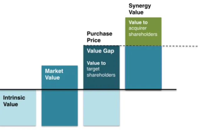
case, as the authors proved, their gains diminish over time and tend to be neutral. Figure 5 graphically represents the distribution of the value created by a deal between two companies. As it is represented, the purchase price turns out to get extremely important, as it influences the value generated to the acquirer’s shareholders. Therefore, even within a deal with positive synergies associated, the acquirer company should never overpay them in order to preserve value for its shareholders.
Figure 5: How the value may be distributed by shareholders between the two parts (Eccles et al.,1999)
2.2.5 Conclusion
M&A is, without doubt, a controversial topic that draws attention for research and debate. Far from being an unanimous topic, the truth is that M&A not only involve metrics – through valuation techniques, which often add subjectivity to the assumptions – but also some dose of unpredictable variables such as emotional attachment, excitement and desire for control (Eccles et al., 1999) .
Through Bruner (2005) and Sirower & Sahni (2006), one can see the reason why M&A transactions saw an upward trend from the late 20th century, despite the prophecies of failure of some literature. If the effects are taken on a macro level, M&A are considered to have a positive impact over the economy as a whole, since the gains absorbed by the target shareholders are greater than the acquirer shareholders’ losses. However, within academics is still possible to sense some distrustfulness about M&A as a tool for generation of value, as the focus and attention predominantly lay on acquirer shareholders’ apparent loss of wealth.
Therefore, it is difficult to determine M&A net benefits for all the agents involved and to the economy as a whole and its inconclusive outcome should be the base of further and more up-to-date research. Current economic times may be unique for M&A field, as companies continue to find more ways to operate and compete efficiently in order to weather harsh economic times as those faced in late 2007. Indeed, efficiency-driven mergers and acquisitions during low economic cycles may create better scenarios for the involved parts than those that have not engaged in such agreements.
Value to acquirer shareholders! Value Gap! ! Value to target shareholders! ! Market Value! Intrinsic Value! Purchase Price! Synergy Value!
3. Company and Industry Analysis
3.1 Airline Industry overview
The airline industry is surely one of the most important sectors for the US economy, with operating revenues of roughly $191 billion in 2011, which is equivalent to 1% of the total GDP of this country. Moreover, the industry not only is a source of economic dynamism – by having carried 730 million passengers in 2011 (Appendix 4) – but also a source of employment, seeing that in the same year it has directly employed 536 000 workers (US Department of Transportation FAA, 2011).
The development of the industry per se is not exclusive to the US and since the second half of the last century global air traffic has exponentially grown. Technological breakthroughs and sustainable increases in the disposable income are considered to be the base of such rapid growth, which helped the airline industry to be one of the major drivers for the globalization trend we live nowadays.
In 1978, following the government’s decision to stop controlling the airfares, routes and new-market entries the US airline sector has been operating in a deregulated market. Ever since, the sector saw unstable periods characterized by a cyclical financial performance that forced the emergence of both bankruptcy and mergers & acquisitions processes.
One considers the past decade as the horribilis period of the global airline industry, with the US industry being particularly affected. Starting the analysis in 2000, 2006 was the first year the industry ran into positive operating results after 9/11 events and 5 consecutive years delivering negative results, accumulating more than $25 billion in losses. In spite of some evidences of recovery, 2008 brought the industry down again specially propelled by the high historic record of jet fuel price - which reached a high historical figure of $3.89 per gallon - and by the economic crisis, which made the American economy halt: in 2008 and 2009 US GDP recorded a negative grow of -0.4% and -3.5% respectively (US Department of Transportation FAA, 2011).
!
!
Figure 6: Domestic Operating Profit and Loss of Major US Major Airlines, Bureau of Transportation Statistics
Indeed, the historical behavior of the industry’s operating results reflects the extremely high industry’s sensitivity not only to internal forces but also to various external factors. Nowadays, companies operate under a highly stressed internal environment. Competition is fierce – and is propelled by low-cost carriers – meaning that one’s company ought to work in a very efficient way; suppliers are few (e.g. Boeing and Airbus are the main
$(10) $(5) $- $5 $10 2000 2001 2002 2003 2004 2005 2006 2007 2008 2009 2010 2011 Billions ($)