www.soil-journal.net/1/459/2015/ doi:10.5194/soil-1-459-2015
© Author(s) 2015. CC Attribution 3.0 License.
SOIL
Evaluation of vineyard growth under four irrigation
regimes using vegetation and soil on-the-go sensors
J. M. Terrón1, J. Blanco2, F. J. Moral2, L. A. Mancha1, D. Uriarte1, and J. R. Marques da Silva3,4,5
1Centro de Investigaciones Científicas y Tecnológicas de Extremadura (CICYTEX) – Instituto de Investigaciones Agrarias Finca “La Orden-Valdesequera”, Gobierno de Extremadura,
Autovía A-5 p.k. 372, 06187, Guadajira (Badajoz), Spain
2Universidad de Extremadura, Escuela de Ingenierías Industriales, Departamento de Expresión Gráfica, Avda. de Elvas, s/n, 06071, Badajoz, Spain
3Universidade de Évora, Instituto de Ciências Agrárias e Ambientais Mediterrânicas (ICAAM), Escola de Ciências e Tecnologia, Apartado 94, 7002-554, Évora, Portugal
4Applied Management and Space Centre for Interdisciplinary Development and Research on Environment (DREAMS), Lisbon, Portugal
5Centro de Inovação em Tecnologias de Informação (CITI), Évora, Portugal Correspondence to: J. M. Terrón (jose.terron@gobex.es)
Received: 15 October 2014 – Published in SOIL Discuss.: 25 November 2014 Revised: 18 May 2015 – Accepted: 3 June 2015 – Published: 17 June 2015
Abstract. Precision agriculture is a useful tool to assess plant growth and development in vineyards. The present study focused on spatial and temporal analysis of vegetation growth variability, in four irrigation treatments with four replicates. The research was carried out in a vineyard located in the southwest of Spain during the 2012 and 2013 growing seasons. Two multispectral sensors mounted on an all-terrain vehicle (ATV) were used in the different growing seasons/stages in order to calculate the vineyard normalized difference vegetation index (NDVI). Soil apparent electrical conductivity (ECa) was also measured up to 0.8 m soil depth using an on-the-go geophysical sensor. All measured data were analysed by means of principal component analysis (PCA). The spatial and temporal NDVI and ECa variations showed relevant differences between irrigation treatments and climatological conditions.
1 Introduction
Terroir is a French concept that means that “there are unique aspects of a place that shape the quality of grapes and wine”. Those aspects that impact on grapes and wine quality are usu-ally associated with topography, soil, climate, plant manage-ment and plant genetics (Vaudour, 2002). According to sev-eral authors, the study of plant vegetative vigour is an essen-tial parameter to successfully manage yield and grape/wine quality because plant growth integrates climate, soil, topog-raphy, available water and other plant controlling factors (Carbonneau, 1995; Cortell et al., 2005; Deloire et al., 2005; Smart, 1985). Consequently, appropriate management of soil and consideration of the main climatic variables are key fac-tors to obtain good yields and, ultimately, quality wines.
Vineyard canopy management practices such as pruning sys-tems, shoot orientation, shoot thinning or leaf removal, have the capacity to modify climate factors around the plant and, consequently, to modify grape and wine quality (Dry, 2000). Vineyard behaviours with regard to water management have been studied in recent decades in a wide range of envi-ronments and vineyard varieties because of the implications of irrigation on yield and quality of the final product (Smart and Coombe, 1983; Williams and Araujo, 2002; Mullins et al., 1992; Bravdo and Hepner, 1986; Intrigliolo and Castel, 2010). Previous authors also indicate that vine vegetative de-velopment is highly influenced by water availability, to the extent that this may become a limiting factor. However, with the same irrigation depth, sometimes the response between
two close plants is not the same. This point should be consid-ered when selecting methods to estimate crop water status in order to achieve better management and to meet the produc-tion objectives defined at the beginning of the growing sea-son. On the one hand, covering all water needs is not recom-mended because this creates management problems, reduces crop quality and in general increases unnecessarily the cost of cultivation. On the other hand, increasing water availabil-ity to the vineyard causes not only grape production to rise, but also the costs of pruning and plant protection treatments, and usually results in reduction of grape quality. Thus, water stress has to be controlled to achieve good yield and qual-ity of grapes as well as balanced growth while avoiding the problems of excess water. It is essential, therefore, to know the correct way to manage this crop.
Several studies related to spectral vegetation indices (VIs) have carried out analyses of vine canopy, shape, size and functional capacity in order to determine spatial and tem-poral management of vegetation as well as other produc-tions factors such as water. Spectral VIs are able to predict a large number of plant features, such as leaf area index (LAI), vegetation fraction cover, fraction of absorbed photosyntheti-cally active radiation (fAPAR), chlorophyll pigment concen-tration, plant stress and other related parameters (Baret and Guyot, 1991; Gitelson and Merzlyak, 2004; Jordan, 1969; Peñuelas et al., 1993; Rondeaux et al., 1996). These VIs, which are mathematical combinations of two or more plant reflectances at specific wavelengths, can be used in vine growth site-specific management enabling the optimization of grape quality and yield (Lamb and Bramley, 2001).
Nowadays, it is possible to obtain a plant spectral signature with a multispectral proximal sensor (Tardáguila and Diago, 2008) suitable for studying vine vegetation terroir. The nor-malized difference vegetation index (NDVI), developed by Rouse et al. (1973), is one of the most extensive indices used for vegetation growth analysis. It can be calculated as
NDVI =NIR − Red
NIR + Red, (1)
where Red and near infra-red (NIR) are the reflectance parameters in the red and NIR electromagnetic radiation bands, respectively. When electromagnetic radiation (natu-ral or man-made) impacts on living green leaves, part of it is absorbed, another part is transmitted and the rest is re-flected. The electromagnetic radiation spectral range that can be absorbed by plants is the photosynthetically active radia-tion (PAR), and is between 0.4 and 0.7 µm (similar to visible range). Within this range, chlorophyll is efficient at capturing the red and blue ranges, and it normally reflects the green, the infrared (IR) and the NIR ranges. Thus, on the basis of NDVI, the greater the amount of vegetative cover or canopy, the higher the value in the index. However, the ability to ab-sorb and reflect both bands depends not only on health plant status but also on plant size. Thus, a plant with water stress, or any other kind of stress (pests, disease, nutritional
defi-ciencies, etc.), will have less capacity to absorb the red band through photosynthetic apparatus and to reflect the NIR band on the cell walls, and will consequently have a lower NDVI value. Therefore, expression of vineyard vegetative develop-ment can be related to NDVI. Several studies have shown the relationship between vegetative canopy parameters, such as LAI and fAPAR, and physiological factors, such as crop production and grape quality, in harvest or plant water status (Smart and Coombe, 1983; Jackson et al., 1983; Dry, 2000). Furthermore, NDVI is also largely related to density of the vegetative canopy of the vineyard (Dobrowski et al., 2002; Johnson, 2003; Hall et al., 2008), so that any change in the factors affecting growth and vineyard development could be estimated by NDVI.
Terroir is also affected by physical, chemical and biolog-ical soil properties; as a tool to interpret these soil property variations, soil apparent electrical conductivity (ECa) may be used. Soil ECa measurements can characterize soil spa-tial variability, with regard mainly to the physical features of the soil, and have been used by other authors to delineate ho-mogeneous management zones (Terrón et al., 2013; Corwin and Lesch, 2003; Moral et al., 2010). Soil ECa measurements can be obtained through geoelectric sensors and this can be an easy and economical way of sampling the soil and guiding soil evaluators in their soil property analyses (Terrón et al., 2011).
According to Hall et al. (2002) the implementation of vine-yard site-specific tools are needed in order to better manage vineyards. Thus, the present work makes use of precision agriculture tools to determine (i) the effects of different irri-gation treatments on vine vegetation growth in two different climatic seasons and (ii) influence of the soil on vegetation growth expression.
2 Material and methods
2.1 Study area and experimental design
The study was carried out during the 2012 and 2013 growing seasons, in a field belonging to the Agrarian Research In-stitute “La Orden – Valdesequera”, in Extremadura (Spain) (38◦510N, 6◦400E). The climate is characterized by mild winters and hot summers, with maximum temperatures reaching 40◦C. Rainfall is irregular, with dry summers and often with an annual average below 500 mm.
The study area is located in a vineyard of 1.8 ha, varietal Tempranillo (Vitis vinifera L.) grafted on Richter 110. It was planted in 2001 by vertical trellis in bilateral cordon system, with 0.6 m stem height and 12 buds per plant. Cultivar Tem-pranillo is a vigorous variety adaptable to all types of soils, preferably slightly acid, and oriented towards areas with a high number of hours of sun per year.
The field is situated in the Guadiana River valley, whose soil morphology is typical of the Quaternary, carved in Ter-tiary sediments. Surface horizons have been artificially
trans-formed for agricultural use with water management, which has resulted in destruction of these horizons and in burial of diagnostic horizons, even below 50 cm. These latter horizons are not differentiated and they have evolved edaphically from the sediments and materials of the lower terraces of the Gua-diana River, which cover the coarser sediments. According to Soil Survey Staff (2006), the soil is in the order Entisol, suborder Orthent and the great group Xerorthent (Xeric).
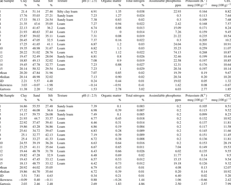
There exists a soil study consisting of a 15-point database randomly distributed on the study area. Tables 1a and 1b show statistic values of soil samples of some physicochemi-cal parameters at two depths (from 0 to 0.30 m and from 0.30 to 0.60 m respectively) which were analysed by official lab-oratory procedures.
From our measurements of a nearby well, we verified that there exists a water table placed at a depth of 6 m, in accor-dance with the river water level. However, from our expe-rience in this area, we know that the level can vary due to rainfall and water use for irrigation.
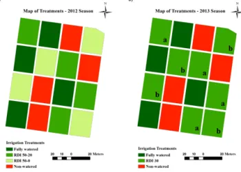
The experimental design was randomized complete blocks, with four replicates (plots) per treatment. Each plot had 108 vines in 6 rows with 18 vines per row, where the distance between plants and rows were 1.20 and 2.50 m re-spectively, placed on a trellis with an east–west row direc-tion. Water treatments were dependent on the growing season (Fig. 1):
i. 2012 treatments were divided into four levels of irriga-tion, corresponding to four levels of crop evapotranspi-ration (ETc) rates:
a. fully watered, based on the application of 100 % ETc;
b. regulated deficit irrigation (RDI) 50-20, based on the regulated deficit irrigation technique, with 50 % ETc before véraison and 20 % ETc after it; c. RDI 50-0, based on the regulated deficit irrigation
technique, with 50 % ETc before véraison and 0 % ETc after it;
d. non-watered, based on rainfed treatment; and ii. 2013 treatments were reduced to three levels of
irriga-tion, corresponding to three levels of ETc rates: a. fully watered, based on the application of 100 %
ETc;
b. RDI 30, based on the regulated deficit irrigation technic, with 30 % ETc throughout the season; and c. non-watered, based on rainfed treatment.
The irrigation system was set up by drip irrigation with one emitter of 4 L h−1every 0.60 m (two emitters per vine) attached to a wire suspended 0.40 m above the ground. Full ETc was calculated by means of the weight differences recorded on a weighing lysimeter installed in the centre of the
Figure 1.Maps of treatments and respective plots: (a) map of treat-ments of 2012 growing season; (b) map of treatment of 2013 grow-ing season, where “a” and “b” replicates of RDI 30 are in the same emplacement of the respective replicates of RDI 20 and RDI 50-0 of the previous season.
assay, corresponding to a fully watered treatment plot (Yris-sarry and Naveso, 1999). Two grapevine plants were planted in the lysimeter container in order to provide the water bal-ance as their canopy developed. Precipitation was collected by an agro-meteorological station located in a reference field near the vineyard.
Soil management was characterized by two annual culti-vator treatments: one in winter dormancy and another at the bud break phenological stage. Later, spontaneous vegetation was controlled by herbicide treatments and 250–350 kg ha−1 of NPK fertilization (9-18-27) was added to the soil. With re-gard to canopy management, a spring pruning was performed to adjust the potential yield to the 12 initial shoots. Subse-quently, before the véraison stage, growing shoots were in-troduced into the trellis to facilitate the passage of agricul-tural machinery. From véraison to harvest, plant protect treat-ments were made against cryptogamic diseases in cycles of 15 to 20 days.
2.2 Vegetation index and soil apparent electrical conductivity
The NDVI estimation was performed with two active proxi-mal multi-spectral sensors mounted on an all-terrain vehicle (ATV). These sensors (OptRx ACS-430, Ag Leader Tech-nology, USA) report directly the vineyard canopy NDVI calculated with red (0.67 µm) and NIR (0.78 µm) wave-lengths. Data sets were collected using a personal digital assistant (PDA) data logger connected to the sensors with TopView software (Betop Topografía SL, Seville – Spain). Geographical coordinates were obtained by a dual-frequency global positioning system (GPS) (GGD Maxor JAVAD Javad GNSS Inc., USA) with real-time kinematic (RTK) differen-tial corrections that reached a planimetric accuracy lower
Table 1.(a) Soil composition from 0 to 0.30 m of the vineyard assay. (b) Soil composition from 0.30 to 0.60 m of the vineyard assay.
(a) Sample Clay Sand Silt Texture pH (1 : 2.5) Organic matter Total nitrogen Assimilable phosphorus Potassium (K+) CEC
% % % % % ppm meq (100 g)−1 meq (100 g)−1
1 21.4 51.14 27.46 Silty clay loam 6.91 1.35 0.038 22.93 0.164 8.82
2 17.76 55.03 27.21 Sandy loam 7.23 1.27 0.024 0.3 0.113 7.64 3 17.33 58.13 24.54 Sandy loam 7.38 0.83 0.02 0.3 0.109 7.68 4 21.35 43.6 35.05 Loam 7.27 0.94 0.022 2.42 0.168 7.57 5 22.13 41.67 36.2 Loam 6.74 0.88 0.013 15.09 0.171 8.24 6 21.93 40.63 37.44 Loam 7.13 0 0.014 7.26 0.159 9.45 7 25.87 39.02 35.11 Loam 7.31 0.08 0.019 21.22 0.235 10.54 8 20.45 47.05 32.5 Loam 7.37 0.16 0.022 0.3 0.205 10.2 9 17.25 41.65 41.1 Loam 6.87 1.2 0.03 24.04 0.201 10.91 10 19.35 48.98 31.67 Loam 6.82 1.3 0.03 35.23 0.259 11.07 11 20.22 51.02 28.76 Loam 6.72 1.12 0.022 74.13 0.268 10.87 12 19.47 52.49 28.04 Sandy loam 6.81 0.8 0.026 32.46 0.199 10.44 13 18.85 49.13 32.02 Loam 7.08 0.9 0.019 22.58 0.197 10.85 14 19.45 47.78 32.77 Loam 7.23 0.88 0.027 12.31 0.176 10.64 15 20.14 50.32 29.54 Loam 7.23 1 0.029 20.34 0.197 10.14 Mean 20.20 47.84 31.96 7.07 0.85 0.02 19.39 0.19 9.67 Median 20.14 48.98 32.02 7.13 0.90 0.02 20.34 0.20 10.20 SD 2.21 5.57 4.48 0.24 0.44 0.01 19.02 0.05 1.32 Skewness 3.03 −0.07 −1.98 −0.14 −0.91 0.41 1.62 0.08 −0.67 Kurtosis 11.38 2.20 7.62 1.53 2.78 3.02 6.03 2.77 1.85
(b) Sample Clay Sand Silt Texture pH (1 : 2.5) Organic matter Total nitrogen Assimilable phosphorus Potassium (K+) CEC
% % % % % ppm meq (100 g)−1 meq (100 g)−1 1 16.86 55.55 27.48 Sandy loam 7.39 0.1 0.003 0.2 0.105 8.51 2 17.32 46.08 36.6 Loam 6.98 0.39 0.007 0.2 0.115 9.52 3 14.17 59.75 26.08 Sandy loam 7.49 0.1 0.005 0.2 0.099 8.23 4 21.93 44.7 33.37 Loam 6.77 0.45 0.018 0.2 0.132 10.92 5 22.92 37.67 39.41 Loam 6.46 0.31 0.014 0.2 0.137 11.81 6 19.86 43.28 36.86 Loam 6.86 0.19 0.004 0.2 0.117 11.58 7 25.61 34.72 39.67 Loam 6.83 0.28 0.009 0.2 0.145 11.66 8 25.1 32.77 42.13 Loam 7.19 0.39 0.009 0.2 0.151 11.45 9 25.4 33.27 41.33 Loam 6.72 0.38 0.008 0.2 0.136 11.81 10 24.55 39.19 36.26 Loam 6.63 0.64 0.016 0.2 0.153 28.19 11 23.25 41.11 35.64 Loam 6.67 0.65 0.011 7.04 0.149 19.53 12 19.44 48.78 31.78 Loam 6.43 0.66 0.026 6.02 0.135 9.55 13 19.82 47.28 32.9 Loam 6.48 0.69 0.02 11.77 0.14 9.5 14 19.43 47.45 33.12 Loam 6.57 0.53 0.012 15.15 0.134 9.54 15 18.13 48.75 33.12 Loam 6.42 0.73 0.012 19.18 0.126 9.32 Mean 20.92 44.02 35.05 6.79 0.43 0.01 4.08 0.13 12.07 Median 19.86 44.70 35.64 6.72 0.39 0.01 0.20 0.14 10.92 SD 3.51 7.81 4.63 0.34 0.21 0.01 6.40 0.02 5.20 Skewness −0.09 0.40 −0.11 0.88 −0.26 1.44 1.06 −0.66 2.42 Kurtosis 2.03 2.46 2.48 2.69 1.83 4.86 2.50 2.57 7.99
than 0.03 m. To obtain vineyard canopy reflectance the ac-tive multi-spectral sensors were placed in nadir position and at a distance, from the top of the grapevines rows, of 0.80 m (±0.20 m, depending on the vineyard height) (Fig. 2). The number of intra-year spectral data sets was fixed to 5 and, according to the season: (i) in 2012, they were started on 29 May and ended on 6 September; and (ii) in 2013, they were started on 30 May and ended on 2 September.
To validate the NDVI with the LAI, several measurements of the latter were taken throughout the ripening stage of the crop in both years. Measurements were recorded by a Plant Canopy Analyser LAI-2000 (LI-COR, Inc, USA), following the procedure of Mabrouk and Carbonneau (1996).
ECa measurements were conducted on 18 February 2011, with a VERIS 3150 Surveyor sensor (Fig. 3), simultaneously in two different soil levels: (i) shallow or ECs – to a depth of 0.30 m from the soil surface; and (ii) deep or ECd – to a depth
of 0.80 m from the surface. Sampling details can be found in Moral et al. (2010).
2.3 Geostatistical and statistical processing
The samplings shown in this work, corresponding to each data set of both growing seasons, were statistically anal-ysed by means of ArcGIS v.10.1 software (ESRI, USA) for geostatistical analyses, and SPSS v.17 software (SPSS Inc., USA), for inferential statistics analyses.
The geostatistical analysis of the multi-temporal NDVI samplings included the followings phases:
i. Voronoi map – a previous exploratory analysis of the samplings was performed to extract outliers.
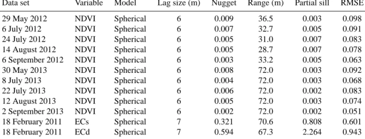
ii. ordinary Kriging interpolation – the parameters used in the semivariograms of each sampling to generate the corresponding maps are shown in Table 2. Once
ob-Table 2.Parameters corresponding to the theoretical semivariograms for the NDVI samplings in 2012 and 2013 growing seasons and for the CEa samplings in 2011 growing season.
Data set Variable Model Lag size (m) Nugget Range (m) Partial sill RMSE
29 May 2012 NDVI Spherical 6 0.009 36.5 0.003 0.098
6 July 2012 NDVI Spherical 6 0.007 32.7 0.005 0.091
24 July 2012 NDVI Spherical 6 0.005 31.0 0.007 0.083
14 August 2012 NDVI Spherical 6 0.005 28.7 0.007 0.078
6 September 2012 NDVI Spherical 6 0.003 33.2 0.005 0.063
30 May 2013 NDVI Spherical 6 0.008 72.0 0.003 0.092
8 July 2013 NDVI Spherical 6 0.004 72.0 0.003 0.068
22 July 2013 NDVI Spherical 6 0.006 72.0 0.002 0.083
12 August 2013 NDVI Spherical 6 0.005 72.0 0.003 0.074
2 September 2013 NDVI Spherical 6 0.002 72.0 0.002 0.051
18 February 2011 ECs Spherical 7 0.321 70.6 0.808 0.601
18 February 2011 ECd Spherical 7 0.594 67.3 2.264 0.943
Figure 2.ATV with two multi-spectral sensors for NDVI mapping of vineyard canopy.
tained, these maps were rasterized using a pixel size of 2 m.
iii. principal component analysis (PCA) – in this work, a PCA process was established separately for each of the years of study.
At each analysis, input raster data set included the five NDVI samplings of the growing seasons, and the output data were distributed in five principal components. Thus, the results of the PCA analyses obtained consisted of five principal com-ponents for each year, where the first principal component shows the NDVI spatial variability for all the mapping dates of each year.
Meanwhile, the ECa samplings were also geostatistically analysed. In this case, only the ordinary Kriging interpolation tool was used, from which the ECs and ECd maps of 2011 were obtained. The parameters used to interpolate the ECa samplings are also shown in Table 2.
Figure 3.Mobile sensor platform Veris 3150 for ECa mapping.
The NDVI samplings from both growing seasons and the ECa samplings at both depths acquired by Kriging were sta-tistically analysed in two phases: (i) firstly, descriptive pa-rameters of each water treatment at each sampling date were acquired to obtain global knowledge of the behaviour of each of the components that make up the statistical design; (ii) sec-ondly, variance analyses of each treatment at each sampling date were made. These analyses allowed comparison of the previously mentioned spatial and temporal behaviours.
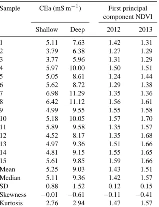
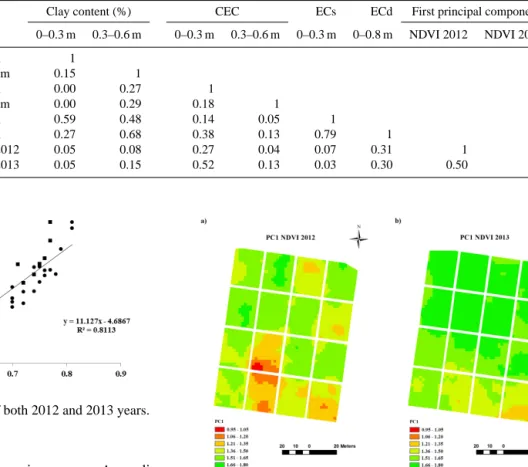
To analyse relationships among all the variables studied, values of the first principal component (PC1) of the NDVI variables in both sampling sequences (years 2012 and 2013) and of ECa (ECs and ECd) in the sampling points from the raster maps (Figs. 6 and 7) were extracted and are shown in Table 3.
Finally, in order to determine the importance of the local soil characteristics, given by the ECa and NDVI parameters respectively, in the vegetative expression of the vineyard, the
Figure 4.(a) Accumulation of rainfall and ETc of 2012 and 2013 growing seasons. (b) Temperature components recorded in both 2012
and 2013 growing seasons: Tmean, Tmax and Tmin are monthly average, maximum and minimum temperature respectively; GDD is the growing degree day reached the last day of the month.
Table 3.CEa, shallow and deep, and first principal component of the NDVI at soil sample localizations.
Sample CEa (mS m−1) First principal
component NDVI Shallow Deep 2012 2013 1 5.11 7.63 1.42 1.31 2 3.79 6.38 1.27 1.29 3 3.77 5.96 1.31 1.29 4 5.97 10.00 1.50 1.51 5 5.05 8.61 1.24 1.44 6 5.62 8.72 1.29 1.38 7 6.98 11.29 1.35 1.36 8 6.42 11.12 1.56 1.61 9 4.99 9.55 1.55 1.58 10 5.18 10.05 1.57 1.70 11 5.89 9.58 1.35 1.57 12 4.52 8.17 1.35 1.68 13 4.97 9.36 1.51 1.66 14 4.81 9.15 1.55 1.65 15 5.61 9.85 1.59 1.66 Mean 5.25 9.03 1.43 1.51 Median 5.11 9.36 1.42 1.57 SD 0.88 1.52 0.12 0.15 Skewness −0.01 −0.61 −0.11 −0.41 Kurtosis 2.76 2.94 1.47 1.57
geographically weighted regression (GWR) tool, included in ArcGIS v.10.1 software (ESRI, USA), was used. The rela-tionship between both variables resulted in maps of deter-mination coefficient (R2) of each water treatment, growing season and depth. The chosen geometric resolution was of 4 m of spatial resolution, which led to goodness of fit in the influence of soil characteristics on the vegetative growth of vines in each of the irrigation treatments of the assay.
3 Results and discussions
Climatic variables logged by the weather station situated in a reference field near the tested vineyard recorded diverse
behaviour during the 2-year test, with drier conditions in the first growing season. Figure 4a and b show cumulative annual rainfall, cumulative annual ETc, temperature parameters and growing degree days (GDDs) on both years. Focusing on the accumulation of precipitation, the total amount in the sec-ond year trial (2013) was more than double compared to the first year trial, where only in its first quarter it had the same amount of rainfall as the whole previous season. However, during the final stages of vegetative development and in the whole ripening phenologic stages, both years had a similarly low accumulation of precipitation. In fact, the temperature was not very different between both years. The observed cli-matological differences in both seasons influenced differen-tially the vineyard vegetative development with respect to the different irrigation treatments analysed in this study.
Despite the large difference in precipitations between the two growing seasons, however, for the second year of the test, which was the wettest, hydric demand was similar to the previous year. This result permitted comparison of vegetative response of two consecutive years that were very different in their climatology. Furthermore, if this premise remains con-stant over the years, it could be possible to know the total needs of the culture of vineyards under whatever climatolog-ical conditions, and appropriate reductions could be made in ETc for a watering schedule based on precipitation occurring at each moment of the campaign. Obviously, as Wample and Smithyman (2002) have reported, increases in hydric neces-sities at each phenological stage must be taken into account, as shown in the slope changes of the accumulation curve of ETc (Fig. 4a), and care must be taken in dry seasons not to bring about unwanted water stress.
In this study, Fig. 5 shows the relationship between LAI estimations and NDVI measurements at the ripening stage of grapes in both years. It can be confirmed that they are well re-lated (R2=0.81), thus indicating the possibility to estimate the degree of development of vineyard crops by NDVI de-terminations obtained by proximal active sensors. These re-sults are in agreement with several authors who have found a good NDVI–LAI relationship (Johnson, 2003).With regard to temporal variability, Fig. 6 shows the results obtained in the first principal component (PC1) of each PCA made on the
Table 4.Correlation matrix (R2) among properties and vegetative vigour expression of the vineyard assay area.
Clay content (%) CEC ECs ECd First principal component 0–0.3 m 0.3–0.6 m 0–0.3 m 0.3–0.6 m 0–0.3 m 0–0.8 m NDVI 2012 NDVI 2013 Clay content (%) 0–0.3 m 1 0.3–0.6 m 0.15 1 CEC 0–0.3 m 0.00 0.27 1 0.3–0.6 m 0.00 0.29 0.18 1 ECs 0–0.3 m 0.59 0.48 0.14 0.05 1 ECd 0–0.8 m 0.27 0.68 0.38 0.13 0.79 1
First principal component NDVI 2012 0.05 0.08 0.27 0.04 0.07 0.31 1
NDVI 2013 0.05 0.15 0.52 0.13 0.03 0.30 0.50 1
Figure 5.NDVI–LAI relationship of both 2012 and 2013 years.
different mapping dates in each growing season. According to these results, there were differences in plant development even when the same doses of irrigation and cultural practices were administered to the plots with different types of irriga-tion treatment.
Soil properties, spatial variation of ECa, both ECs and ECd, and PC1 of NDVI (both 2012 and 2013 growing sea-sons) were statistically analysed (Table 4). On the one hand, ECs and ECd results were correlated with the clay content from 0 to 0.30 m (R2=0.59 and R2=0.27, respectively) and from 0.30 to 0.60 m (R2=0.48 and R2=0.68, respec-tively). These results indicate that ECa could be used as a tool to estimate some soil properties – thus avoiding the time-consuming inconvenience and cost of soil sampling and anal-ysis in the laboratory. On the other hand, it is of interest to note the correlation between CEC, from 0 to 0.30 m, and PC1 of NDVI of 2013 (R2=0.53), indicating the higher influence of soil fertility due to the existence of water resources in that year.
Results of ECa spatial variation (Fig. 7) seem to be a pat-tern consisting of a variation in ECa from the northern and southern boundaries of the assay up to the centre, and also from east to west, coinciding with some physicochemical pa-rameters of soil. There exists, too, a pattern in the variability of soil characteristics due to the good relationship with ECa, in particular with clay content (Moral et al., 2010). Spatial variability of ECa, both shallow and deep, had also shown significant differences among the locations of the plots of the
Figure 6.NDVI first principal component of (a) 2012 and (b) 2013.
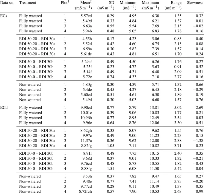
different irrigation treatments (Table 5), with different val-ues for the soil properties that influenced vegetative growth of the grapevines. In general, the spatial variability pattern mentioned above was observed in the plots with the differ-ent treatmdiffer-ents, with higher ECs or ECd values in those plots near the northern and southern boundaries of the vineyard test site. Because of this spatial variability, it was necessary to perform, even within plots of the same treatment, geosta-tistical analyses between NDVI and ECa to determine the ex-tent of the influence of soil properties on vegetative growth of the vineyard in each of the irrigation treatments and their respective plots.
3.1 Intra-year variability 3.1.1 2012 growing season
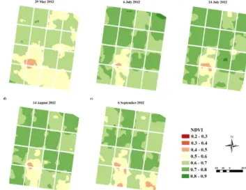
Both temporal and spatial evolution of the NDVI index of the irrigation treatments and their respective plots in the 2012 growing season is shown in Fig. 8. At first glance, the re-sults of NDVI mapping for this year show how all the treat-ments had a temporal evolution similar to a Gaussian func-tion, the mean value of the index increasing as the campaign advanced, reaching a maximum value around the
phenolog-Table 5.Statistic descriptive analyses of shallow and deep soil ECa interpolated data.
Data set Treatment Plot1 Mean2 SD Minimum Maximum Range Skewness
(mS m−1) (mS m−1) (mS−1) (mS m−1) (mS m−1)
ECs Fully watered 1 5.57cd 0.29 4.95 6.30 1.35 0.32
Fully watered 2 5.49d 0.33 4.84 6.21 1.37 0.01
Fully watered 3 6.63a 0.55 5.54 7.69 2.15 −0.02
Fully watered 4 5.94b 0.48 5.05 6.83 1.78 0.16
RDI 50-20 – RDI 30a 1 4.55h 0.17 4.23 5.06 0.83 0.40
RDI 50-20 – RDI 30a 2 5.52d 0.42 4.60 6.75 2.15 −0.08
RDI 50-20 – RDI 30a 3 6.59a 0.30 5.82 7.39 1.57 0.14
RDI 50-20 – RDI 30a 4 5.61de 0.43 4.81 6.51 1.70 0.24
RDI 50-0 – RDI 30b 1 5.29ef 0.49 4.50 6.26 1.76 0.27
RDI 50-0 – RDI 30b 2 5.25f 0.23 4.72 5.63 0.91 −0.52 RDI 50-0 – RDI 30b 3 5.14f 0.49 4.31 6.40 2.09 0.51 RDI 50-0 – RDI 30b 4 5.72c 0.74 4.33 7.10 2.77 −0.16 Non-watered 1 4.80g 0.30 4.39 5.71 1.32 0.66 Non-watered 2 5.4de 0.45 4.27 6.45 2.18 −0.29 Non-watered 3 5.60cd 0.51 4.61 6.50 1.89 0.19 Non-watered 4 5.49d 0.30 5.03 6.60 1.57 0.76
ECd Fully watered 1 9.90cd 0.77 8.79 13.81 5.02 2.69
Fully watered 2 10.01c 0.39 9.06 10.83 1.77 0.21
Fully watered 3 10.96b 0.77 8.95 12.49 3.54 −0.03
Fully watered 4 9.96c 0.64 8.76 12.06 3.30 0.51
RDI 50-20 – RDI 30a 1 8.62gh 0.33 8.07 9.62 1.55 0.76
RDI 50-20 – RDI 30a 2 9.97c 0.49 9.00 11.23 2.23 0.15
RDI 50-20 – RDI 30a 3 11.37a 0.36 9.62 12.00 2.38 −1.38
RDI 50-20 – RDI 30a 4 8.82fg 1.05 7.11 10.82 3.71 0.23
RDI 50-0 – RDI 30b 1 8.91f 0.48 7.75 10.15 2.40 0.35 RDI 50-0 – RDI 30b 2 9.68d 0.37 9.01 10.33 1.32 −0.21 RDI 50-0 – RDI 30b 3 9.76cd 0.48 8.73 10.55 1.82 −0.43 RDI 50-0 – RDI 30b 4 8.88fg 1.51 6.08 11.50 5.42 −0.04 Non-watered 1 8.53h 0.37 7.82 9.47 1.65 0.27 Non-watered 2 9.40e 0.77 7.41 11.14 3.73 −0.20 Non-watered 3 9.77cd 0.28 9.11 10.49 1.38 0.35 Non-watered 4 8.72fgh 0.57 7.90 10.53 2.63 0.99
Sampling was carried out on 18 February 2011.1Plots are numbered in a north–south orientation.2Variance analyses among treatments are made for each data set independently; a, b, c, and d mean significant difference at p value ≤ 0.05 in Tukey post hoc analysis.
ical stage of véraison, and then decreasing until harvest. In spite of this sigmoidal evolution, a positive relationship be-tween NDVI and water dose occurred, in which the fully wa-tered treatment maintained the higher mean value of NDVI, and the non-watered treatment the lower mean value, for all the mapping dates, these differences being, moreover, sig-nificant (Table 6). These results indicate that the greater the quantity of water in the vineyard the higher the vegetative development of its canopy.
The intermediate RDI 50-20 and RDI 50-0 irrigation treat-ments also showed significant differences between NDVI values with regard to the previous ones, with intermediate values. Both RDI treatments kept their NDVI values similar
up to January, and then they became different as a result of the change in the water dose of the experimental design. At that moment, the RDI 50-0 treatment had a greater decrease in NDVI mean value and, consequently, in vegetative expres-sion of the vineyard. Taking into account these aspects, and bearing in mind the existing relationship between vegetative growth of the vines and NDVI value, it can be considered that the latter increased its value when water doses were higher, and that variations in doses will result in changes in the veg-etative expression of the vineyard.
On the other hand, despite the relation found between the water doses applied in the assay and the vegetative develop-ment of the vines, there were significant differences among
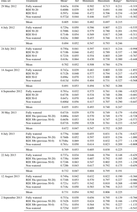
Table 6.Statistic descriptive analyses of the NDVI interpolated data sets for 2012 and 2013 growing seasons (dimensionless).
Data set Treatment Mean1 SD Minimum Maximum Range2 Skewness
29 May 2012 Fully watered 0.643a 0.036 0.502 0.713 0.211 −0.319
RDI 50-20 0.608b 0.039 0.507 0.691 0.184 −0.548
RDI 50-0 0.597c 0.046 0.472 0.706 0.234 −0.265
Non-watered 0.572d 0.044 0.446 0.677 0.231 −0.302
Mean 0.605 0.041 0.482 0.697 0.215
6 July 2012 Fully watered 0.729a 0.050 0.586 0.807 0.221 −0.535
RDI 50-20 0.708b 0.042 0.579 0.780 0.201 −0.591
RDI 50-0 0.714b 0.054 0.569 0.817 0.248 −0.311
Non-watered 0.624c 0.060 0.453 0.766 0.313 −0.210
Mean 0.694 0.052 0.547 0.793 0.246
24 July 2012 Fully watered 0.750a 0.041 0.597 0.813 0.216 −0.998
RDI 50-20 0.718b 0.046 0.452 0.789 0.337 −1.300
RDI 50-0 0.721b 0.055 0.554 0.803 0.249 −0.767
Non-watered 0.618c 0.064 0.430 0.730 0.300 −0.448
Mean 0.702 0.052 0.508 0.784 0.276
14 August 2012 Fully watered 0.742a 0.039 0.483 0.803 0.320 −1.853
RDI 50-20 0.712b 0.048 0.577 0.794 0.217 −0.475
RDI 50-0 0.696c 0.070 0.512 0.800 0.288 −0.828
Non-watered 0.613d 0.054 0.404 0.731 0.327 −0.568
Mean 0.691 0.053 0.494 0.782 0.288
6 September 2012 Fully watered 0.701a 0.032 0.575 0.761 0.186 −0.825
RDI 50-20 0.673b 0.045 0.534 0.740 0.206 −0.681
RDI 50-0 0.647c 0.070 0.445 0.750 0.305 −0.917
Non-watered 0.600d 0.056 0.417 0.707 0.290 −0.647
Mean 0.655 0.051 0.493 0.740 0.247
30 May 2013 Fully watered 0.671b 0.039 0.570 0.749 0.179 −0.454
RDI 30a (previous 50-20) 0.680a 0.045 0.570 0.749 0.179 −0.728 RDI 30b (previous 50-0) 0.665b 0.053 0.518 0.747 0.229 −0.573
Non-watered 0.671b 0.050 0.528 0.761 0.233 −0.547
Mean 0.672 0.047 0.547 0.752 0.205
8 July 2013 Fully watered 0.779a 0.040 0.655 0.831 0.176 −0.827
RDI 30a (previous 50-20) 0.766b 0.052 0.597 0.833 0.236 −1.000 RDI 30b (previous 50-0) 0.754bc 0.069 0.555 0.832 0.277 −1.138
Non-watered 0.761c 0.050 0.614 0.823 0.209 −0.808
Mean 0.769 0.053 0.605 0.830 0.225
22 July 2013 Fully watered 0.737a 0.034 0.646 0.794 0.148 −0.429
RDI 30a (previous 50-20) 0.738a 0.049 0.607 0.792 0.185 −1.200 RDI 30b (previous 50-0) 0.724b 0.063 0.547 0.802 0.255 −1.238
Non-watered 0.728b 0.043 0.617 0.792 0.175 −0.659
Mean 0.732 0.047 0.604 0.795 0.191
12 August 2013 Fully watered 0.749a 0.042 0.632 0.822 0.190 −0.366
RDI 30a (previous 50-20) 0.734b 0.053 0.570 0.797 0.227 −0.986 RDI 30b (previous 50-0) 0.721c 0.071 0.542 0.810 0.268 −0.989
Non-watered 0.718c 0.050 0.583 0.796 0.213 −0.735
Mean 0.731 0.054 0.582 0.806 0.225
2 September 2013 Fully watered 0.753a 0.030 0.656 0.795 0.139 −0.766 RDI 30a (previous 50-20) 0.742b 0.035 0.624 0.790 0.166 −1.076 RDI 30b (previous 50-0) 0.731c 0.054 0.564 0.791 0.227 −1.133
Non-watered 0.725d 0.037 0.609 0.781 0.172 −0.543
Mean 0.738 0.039 0.613 0.789 0.176
1Variance analyses among treatments are made for each data set independently; a, b, c, and d mean significant difference at p value ≤ 0.05 in Tukey post hoc
Figure 7. Interpolated apparent electrical conductivity maps of 2011 growing season: (a) shallow ECa map and (b) deep ECa map.
the various plots of each water treatment (data not shown), indicating that spatial variability of the NDVI index existed, and consequently of vegetative growth too, which was de-pendent on other factors, even though the characteristics of the management were identical. In this respect, it can be ob-served in Fig. 8 how vegetative expression was not homo-geneous in all the plots within a specific water treatment, but rather variations were found in the NDVI value depend-ing on the geographical location of each of the plots. Thus, on a specific mapping date, some plots with different wa-ter treatments had similar mean values of NDVI, even be-tween plots with fully watered and non-watered treatments. A factor associated with geographical location, therefore, has had some influence on the vegetative growth. The terroir ef-fect, in which the physicochemical parameters of soil are in-cluded, could be one of the factors that have caused a cer-tain influence on vegetative development, as indicated by van Leeuwen and Seguin (2006).
A priori, the global results on the relationship between NDVI and ECa indicate a low association when compared in the first 0.30 m of soil depth (ECs, Table 7), and a rel-atively high one when a large section of soil is considered (ECd, Table 7). These results suggest that the soil surface layer has little influence on vegetative expression of the vine-yard because of the deeper distributions of the roots, although it does influence other crops with shallow roots (Fortes et al., 2014). Furthermore, in the year when climatic quality in-volved drought (2012), ECa and NDVI values were lower, suggesting that the soil properties seem to be an influential factor but not a limiting one in vegetative expression, the availability of water resources being the principal limiting factor.
Figure 8. Interpolated NDVI maps of 2012 growing season:
(a) 29 May; (b) 6 July; (c) 24 July; (d) 14 August; and (e) 6
Septem-ber.
Figure 9. NDVI maps year 2013: (a) 30 May; (b) 8 July;
(c) 22 July; (d) 12 August; and (e) 2 September.
3.1.2 2013 growing season
Figure 9 shows the spatial and temporal evolution of NDVI in the watered treatments and their respective plots in the 2013 growing season. In the same way as the previous year, in-creased water doses applied to the vineyard were associated with a higher NDVI mean value. However, in this season, the differences in this mean value were closer, being no higher than 0.10 points of index value. The intense precipitations be-tween post-harvest of 2012 and flowering of 2013 decreased the possibility of water stress in the vines, so vegetative de-velopment was very similar at the beginning of the NDVI mappings, the only difference being the RDI 30 treatment that came from the RDI 50-20 of the previous growing season (Table 6). On the other hand, in the 2013 season, temporal
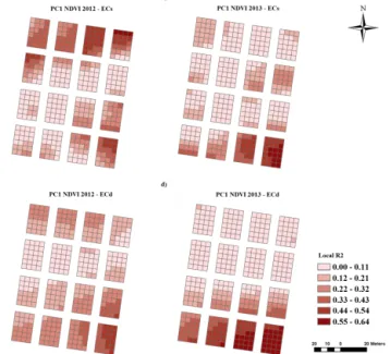
Figure 10.Local R2of GWR analyses: (a) first principal nent of NDVI in 2012 and ECs of 2011; (b) first principal nent of NDVI in 2013 and ECs of 2011; (c) first principal nent of NDVI in 2012 and ECd of 2011; (d) first principal compo-nent of NDVI in 2013 and ECd 2011.
evolution of the mean NDVI value of the whole treatments was more homogeneous for most of the season. Generally speaking, there was an initial increment of the NDVI value in all treatments up to the phenological stage of véraison, from which point that value was constant until the harvest. Both results, i.e. higher and constant NDVI values as com-pared to the previous season, may have been caused by the high groundwater recharge, which provided almost unlimited water to plants during the early stages of vineyard growth.
With regard to temporal behaviour of NDVI between wa-ter treatments, the mean value of the index resulted in slightly higher significant differences as the season progressed, with two different groups of treatments at véraison (Table 6): (i) fully watered and RDI 30a and (ii) non-watered and RD 30b. From this moment until harvest, the irrigation treat-ments of the first group showed significant differences in the mean NDVI value, while treatments of the second group had a similar value. In general, in the same way as the previous season, there were some factors, in this case climatological ones, that modified the expected trend of a vineyard managed under specific water conditions.
The irrigation treatments of the 2013 growing season also had significant differences in mean NDVI values among their respective plots spatially (data not shown), with a pattern of reduced values from north to south of the vineyard test area. Thus, for the same water treatment and mapping date, the mean NDVI values of each plot decreased the further south the plot was located, with, furthermore, significant differ-ences among them. This result was already shown by Blanco
Table 7.Correlation matrix (R2) between first principal compo-nents of 2012 and 2013 growing seasons and apparent electrical conductivities, shallow and deep, interpolated data of 2011.
Variable First PC First PC ECs ECd NDVI 2012 NDVI 2013 2011 2011 First PC NDVI 2012 1.00
First PC NDVI 2013 0.58 1.00 ECs 2011 0.18 0.16 1.00 ECd 2011 0.59 0.70 0.83 1.00
et al. (2012), who reported that vegetative growth of vines under the same management had different behaviours due to spatial changes in some influential factor, such us spatial variability of the physicochemical properties of soil. On the other hand, the influence of terroir, taking into account its climatic and edaphic factors, was so high in the 2013 sea-son that it gave rise to similar mean NDVI values, with some exceptions, in plots with different irrigation treatments. Thus, for example, northern plots of fully watered and non-watered treatments gave similar NDVI values, as did the southern plots, but these values were statistically different between the two geographical locations. This behaviour can be seen in Fig. 9.
Figure 10 shows the local relationship between the PC1 of NDVI in each growing season and the ECa in 2011, both shallow and deep, throughout the test area, which is the level of influence of soil features on vegetative development in each water treatment. The highest ratios prevailed, again, in the northern and southern limits of the test area, in agreement with those zones where ECa reached the lowest values. Thus, the maximum values in the relationship between soil prop-erties and vegetative growth were obtained during the 2013 season; values of R2 in the relationship between soil prop-erties and vegetative growth were obtained during the 2013 season, with values of R2of 0.55 and 0.64 points of ECs and ECd respectively, compared to 0.56 and 0.47 points reached in 2012. Thus, a lower maximum value of ECa was produced in the 2012 growing season. However, that year presented a good relationship between ECa and NDVI in a larger area than the 2013 growing season. These results could be due to the fact that soils with water limits in zones where ECa has low values (and lower expected clay content) (Sudduth et al., 2005; Terrón et al., 2011) tend to have higher water availabil-ity for the plant as compared to soils with higher ECa values (higher percentage of clay content).
3.2 Between-year variability
The results of each mapping date of NDVI in both growing seasons (Figs. 8 and 9) show the behaviour of the vegeta-tive development of the whole treatments established in the experimental designs. As has already been stated, NDVI val-ues and, accordingly, vegetative growth of the vineyard were
Table 8.Correlation matrices between 2012 and 2013 NDVI surfaces of each irrigation treatment. 2012
Treatment Data set 29 May 6 July 24 July 4 August 6 September
Fully watered 29 May 1
6 July 0.47 1 24 July 0.33 0.65 1 14 August 0.42 0.35 0.47 1 6 September 0.28 0.57 0.59 0.57 1 RDI 50-20 29 May 1 6 July 0.74 1 24 July 0.61 0.72 1 14 August 0.69 0.79 0.70 1 6 September 0.70 0.81 0.66 0.84 1 RDI 50-0 29 May 1 6 July 0.59 1 24 July 0.69 0.86 1 14 August 0.69 0.89 0.86 1 6 September 0.68 0.86 0.83 0.95 1 Non-watered 29 May 1 6 July 0.70 1 24 July 0.68 0.83 1 14 August 0.66 0.83 0.81 1 6 September 0.65 0.82 0.79 0.90 1 2013
30 May 8 July 22 July 12 August 2 September
Fully watered 30 May 1
8 July 0.76 1
22 July 0.61 0.61 1
12 August 0.58 0.66 0.67 1
2 September 0.64 0.79 0.63 0.76 1
RDI 30a 30 May 1
8 July 0.85 1 22 July 0.82 0.86 1 12 August 0.83 0.85 0.93 1 2 September 0.83 0.87 0.91 0.90 1 RDI 30b 30 May 1 8 July 0.90 1 22 July 0.87 0.93 1 12 August 0.88 0.94 0.95 1 2 September 0.89 0.95 0.95 0.96 1 Non-watered 30 May 1 8 July 0.80 1 22 July 0.77 0.88 1 12 August 0.84 0.89 0.88 1 2 September 0.73 0.83 0.85 0.86 1
influenced by soil properties (including groundwater level) in spatial components, and by climatic features in temporal ones.
With regard to the temporal variability, Fig. 6 shows the results obtained in the first principal component (PC1) of each PCA made for the different mapping dates in each grow-ing season. This PC1 shows spatial variability of NDVI for
the whole of NDVI mapping dates for each year. Thus, each PC1 map for 2012 explains 80.57 % of the temporal vari-ability of each geographical location within the assay area, and 85.92 % for the 2013 growing season. Thus, the PC1 for each year shows more than 80 % of the mean variability of the NDVI values throughout both seasons in each of the ir-rigation treatments and their respective plots. In general, the PC1 map for 2013 shows higher and more homogeneous val-ues than the 2012 one, indicating a higher and more homo-geneous vegetative growth of grapevines.
Table 8 shows the level of relationship of NDVI values between the different mapping dates for each irrigation treat-ment. Generally speaking, in both 2012 and 2013 there was an increase in the determination coefficient (R2) given by the NDVI values as the season progressed, indicating that the continuous development of the vineyard canopy was slow-ing; that is, the development rate or evolution of that canopy was increasingly smaller until the harvest stage was reached. However, the behaviour of the different irrigation treatments did not evolve equally either within years or between years. In 2012, the treatment with higher water doses (fully wa-tered) had low values of correlation (R2 lower than 0.65) in all NDVI mapping dates due to a higher development rate versus the rest of water and rainfed treatments during the later phenological stages of the vineyard, thus indicating higher change rates. Conversely, Non-watered treatment had determination coefficients above 0.65 points, which suggests a low development rate due to lower hydric availability as a limiting factor. Meanwhile, the 2013 season showed a sim-ilar behaviour pattern in the extreme water treatments. Ob-viously, the determination coefficients were higher and more homogeneous than the previous season between the different mapping dates due to the intense precipitations, these being
R2<0.77 for fully watered and R2>0.73 for non-watered treatments. These results point to a lower canopy develop-ment than in 2012 and, in the 2013 season, the differences between treatments were less pronounced.
With respect to differences in spatial variability of vegeta-tive growth between the years tested, the 2013 season showed greater homogeneity, where the highest increase was found in the northern half of the test area, regardless of the water dose applied. Conversely, this vegetative development was lower in the south, where the southern plot of non-watered treatment did not have lower vegetative growth, although it did respond to a spatial pattern. Thus, the vegetation response in 2012 was more dependent on the irrigation treatments, while in 2013 it was more dependent on soil characteristics or other edaphic–climatic variables. In 2013, RDI 50-20 and RDI 50-0 treatments became RDI 30a and RDI 30b respec-tively, with water doses of 30 % of ETc during the whole irri-gation period. In the same way that the rest of the treatments had higher NDVI values in 2013, RDI 30 also showed higher NDVI values than the RDI treatments of the previous season. However, despite having the same water dose, RDI 30b gave lower values than RDI 30a during most of the season (data
not shown), thus suggesting once again that water dose must be redefined taking into account climate and soil properties.
According to Howell (2001), there must be an optimal method of crop management in any situation, in order to obtain the desired yields and qualities, but intra-year and between-year management must be performed in accordance with the terroir features of each year.
4 Conclusions
Water level and vegetative growth were clearly related; greater availability of water resources gave rise to greater vegetative development of the vineyard. However, spatial– temporal changes in climatic quality or in soil properties also affect vegetative expression. To the already estimated differ-ences in vegetative growth of grapevines between different water doses, one must add the effects that climate and soil properties have on plants. Consequently, the application of the same cultural practices in each growing season makes it unfeasible to attain stable goals, i.e. the same level of qual-ity in grapes and wines or similar yields every season. The application of some precision agriculture techniques to the vineyard crop, through real-time measurements of NDVI and ECa, makes it possible to determine homogeneous zones of growth and development in the vineyard dependent on cli-matic and soil characteristics for a specific irrigation treat-ment. Thus, according to the results of this study, the follow-ing can be concluded:
i. In global terms, the higher the water doses the higher the NDVI values and, hence, the greater the vegetative growth of the vineyard.
ii. Vegetative development is not homogeneous, even when the same cultural practices are being used, but spatial and temporal variability occur depending on cli-matic and soil characteristics and their interactions. iii. It is necessary for crop management to adapt to the
vari-ability of agronomic factors in order to achieve homo-geneous vegetative growth even in zones where the soil characteristics are different.
An irrigation schedule based on real-time NDVI results, and knowledge of the variability of soil characteristics could be the basis for improved vineyard management.
Acknowledgements. This work was carried out with funding from the RITECA Project, Transboundary Research Network Ex-tremadura, Center and Alentejo, co-financed by the European Re-gional Development Fund (ERDF), by the Spain–Portugal Border Cooperation Operational Programme (POCTEP) 2007–2013 and by the Government of Extremadura.
This research was also co-financed by the Government of Ex-tremadura and the European Regional Development Fund (ERDF) through the project GR10038 (Research Group TIC008).
The vineyard irrigation project which has complemented this work is INIA RTA2009-00026-C02-02 and was co-financed by the European Regional Development Fund (ERDF).
Edited by: E. Costantini
References
Baret, F. and Guyot, G.: Potentials and limits of vegetation indices for LAI and APAR assessment, Remote Sens. Environ., 35, 161– 173, 1991.
Blanco, J., Terrón, J. M., Pérez, F. J., Galea, F., Salgado, J. A., Moral, F. J., Marques da Silva, J. R., and Silva, L. L.: Variabili-dad espacial y temporal del vigor vegetativo en viñedo sin restric-ciones hídricas en la demanda evapotranspirativa, VII Congreso Ibérico de Agroingeniería y Ciencias Hortícolas, Madrid, 2012. Bravdo, B. and Hepner, Y.: Irrigation management and fertigation to
optimize grape composition and vine performance, Symposium on Grapevine Canopy and Vigor Management, XXII IHC 206, 49–68, 1986
Carbonneau, A.: General relationship within the whole-plant: exam-ples of the influence of vigour status, crop load and canopy expo-sure on the sink “berry maturation” for the grapevine, Strategies to Optimize Wine Grape Quality 427, 99–118, 1995.
Cortell, J. M., Halbleib, M., Gallagher, A. V., Righetti, T. L., and Kennedy, J. A.: Influence of Vine Vigor on Grape (Vitis vinifera L. Cv. Pinot Noir) and Wine Proanthocyanidins, J. Agr. Food Chem., 53, 5798–5808, 2005.
Corwin, D. and Lesch, S.: Application of soil electrical conductivity to precision agriculture, Agron. J., 95, 455–471, 2003.
Deloire, A., Vaudour, E., Carey, V., Bonnardot, V., and van Leeuwen, C.: Grapevine responses to terroir: a global approach, J. Int. Sci. Vigne Vin, 39, 149–162, 2005.
Dobrowski, S. Z., Ustin, S. L., and Wolpert, J. A.: Remote estima-tion of vine canopy density in vertically shoot-posiestima-tioned vine-yards: determining optimal vegetation indices, Aust. J. Grape Wine R., 8, 117–125, 2002.
Dry, P. R.: Canopy management for fruitfulness, Aust. J. Grape Wine R., 6, 109–115, 2000.
Fortes, R., Prieto, M., Terron, J., Blanco, J., Millan, S., and Campillo, C.: Using apparent electric conductivity and NDVI measurements for yield estimation of processing tomato crop, T. ASABE, 57, 827–835, 2014.
Gitelson, A. A. and Merzlyak, M. N.: Non-Destructive Assessment of Chlorophyll Carotenoid and Anthocyanin Content in Higher Plant Leaves: Principles and Algorithms, in: Remote Sensing for Agriculture and the Environment, edited by: Stamatiadis, S., Lynch, J. M., and Schepers, J. S., Ella, Greece, 78–94, 2004. Hall, A., Lamb, D. W., Holzapfel, B., and Louis, J.: Optical
re-mote sensing applications in viticulture – a review, Aust. J. Grape Wine R., 8, 36–47, 2002.
Hall, A., Louis, J., and Lamb, D. W.: Low-resolution remotely sensed images of winegrape vineyards map spatial variability in planimetric canopy area instead of leaf area index, Aust. J. Grape Wine R., 14, 9–17, 2008.
Howell, G. S.: Sustainable grape productivity and the growth-yield relationship: A review, Am. J. Enol. Viticult., 52, 165–174, 2001. Intrigliolo, D. S. and Castel, J. R.: Response of grapevine cv. “Tem-pranillo” to timing and amount of irrigation: water relations, vine
growth, yield and berry and wine composition, Irrigation Sci., 28, 113–125, 2010.
Jackson, R. D., Slater, P. N., and Pinter Jr., P. J.: Discrimination of growth and water stress in wheat by various vegetation indices through clear and turbid atmospheres, Remote Sens. Environ., 13, 187–208, 1983.
Johnson, L. F.: Temporal stability of an NDVI-LAI relationship in a Napa Valley vineyard, Aust. J. Grape Wine R., 9, 96–101, 2003. Jordan, C. F.: Derivation of Leaf-Area Index from Quality of Light
on Forest Floor, Ecology, 50, 663–666, 1969.
Lamb, D. and Bramley, R. G. V.: Managing and monitoring spa-tial variability in vineyard variability, Nat. Res. Man., 4, 25–30, 2001.
Mabrouk, H. and Carbonneau, A.: A simple method for determina-tion of grapevine Vitis vinifera L. leaf area, Progres Agricole et Viticole, 113, 392–398, 1996.
Moral, F. J., Terrón, J. M., and Marques da Silva, J. R.: Delineation of management zones using mobile measurements of soil appar-ent electrical conductivity and multivariate geostatistical tech-niques, Soil and Tillage Research, 106, 335–343, 2010. Mullins, M. G., Bouquet, A., and Williams, L. E.: Biology of the
Grapevine, Cambridge University Press, 1992.
Peñuelas, J., Filella, I., Biel, C., Serrano, L., and Save, R.: The re-flectance at the 950–970 nm region as an indicator of plant water status, Int. J. Remote Sens., 14, 1887–1905, 1993.
Rondeaux, G., Steven, M., and Baret, F.: Optimization of soil-adjusted vegetation indices, Remote Sens. Environ., 55, 95–107, 1996.
Rouse, J. W., Haas, R. H., Schell, J. A., and Deering, D. W.: Moni-toring the vernal advancement and retrogradation (green wave ef-fect) of natural vegetation, Remote Sensing Center, Texas A&M Univ., College Station, 93 pp., 1973.
Smart, R. E. and Coombe, B. G.: Water relations of grapevines, in: Water deficits and plant growth, edited by: Kozlowski, T. T., Aca-demic Press, 137–196, 1983.
Smart, R. E.: Principles of Grapevine Canopy Microclimate Manip-ulation with Implications for Yield and Quality. A Review, Am. J. Enol. Viticult., 36, 230–239, 1985.
Soil Survey Staff: Keys to soil taxonomy, USDA-Natural Resources Conservation Service, Washington, D.C., 333 pp., 2006. Sudduth, K., Kitchen, N., Wiebold, W., Batchelor, W., Bollero, G.,
Bullock, D., Clay, D., Palm, H., Pierce, F., and Schuler, R.: Relat-ing apparent electrical conductivity to soil properties across the north-central USA, Comput. Electron. Agr., 46, 263–283, 2005. Tardáguila, J. and Diago, M.: Viticultura de precisión: principios
y tecnologías aplicadas en el viñedo, VI World Wine Forum, Logroño, Spain, 2008.
Terrón, J., da Silva, J. M., Moral, F., and García-Ferrer, A.: Soil apparent electrical conductivity and geographically weighted re-gression for mapping soil, Precis. Agric., 12, 750–761, 2011. Terrón, J., Moral, F., da Silva, J. M., and Rebollo, F.: Analysis of
spatial pattern and temporal stability of soil apparent electrical conductivity and relationship with yield in a soil of high clay content, 3rd Global Workshop on Proximal Soil Sensing, 2013. van Leeuwen, C. and Seguin, G.: The concept of terroir in
viticul-ture, Journal of Wine Research, 17, 1–10, 2006.
Vaudour, E.: The Quality of Grapes and Wine in Relation to Ge-ography: Notions of Terroir at Various Scales, Journal of Wine Research, 13, 117–141, 2002.
Wample, R. and Smithyman, R.: Regulated deficit irrigation as a water management strategy in Vitis vinifera production, in: Deficit irrigation practices, Food and Agricultural Organization of the United Nations (FAO), Rome, Italy, 89–100, 2002. Williams, L. E. and Araujo, F. J.: Correlations among Predawn Leaf,
Midday Leaf, and Midday Stem Water Potential and their Corre-lations with other Measures of Soil and Plant Water Status in Vitis vinifera, J. Am. Soc. Hortic. Sci., 127, 448–454, 2002.
Yrissarry, J. J. B. and Naveso, F. S.: Use of weighing lysimeter and Bowen-Ratio Energy-Balance for reference and actual crop evap-otranspiration measurements, III International Symposium on Ir-rigation of Horticultural Crops, 537, 143–150, 1999.