Light field image coding with jointly estimated self-similarity bi-prediction

Deposited in Repositório ISCTE-IUL:

Deposited version:

Peer-review status of attached file:

Citation for published item:

Conti, C., Nunes, P. & Soares, L. D. (2018). Light field image coding with jointly estimated self-similarity bi-prediction. Signal Processing: Image Communication. 60, 144-159

Further information on publisher's website:

Publisher's copyright statement:

This is the peer reviewed version of the following article: Conti, C., Nunes, P. & Soares, L. D. (2018). Light field image coding with jointly estimated self-similarity bi-prediction. Signal Processing: Image Communication. 60, 144-159, which has been published in final form at

https://dx.doi.org/10.1016/j.image.2017.10.006. This article may be used for non-commercial purposes in accordance with the Publisher's Terms and Conditions for self-archiving.

Use policy

Creative Commons CC BY 4.0

The full-text may be used and/or reproduced, and given to third parties in any format or medium, without prior permission or charge, for personal research or study, educational, or not-for-profit purposes provided that:

• a full bibliographic reference is made to the original source • a link is made to the metadata record in the Repository • the full-text is not changed in any way

The full-text must not be sold in any format or medium without the formal permission of the copyright holders. Serviços de Informação e Documentação, Instituto Universitário de Lisboa (ISCTE-IUL)

Av. das Forças Armadas, Edifício II, 1649-026 Lisboa Portugal Phone: +(351) 217 903 024 | e-mail: administrador.repositorio@iscte-iul.pt



_{Light Field Image Coding with Jointly Estimated}

Self-Similarity Bi-Prediction

Caroline Conti

, Paulo Nunes, and Luís Ducla Soares

Abstract

This paper proposes an efficient light field image coding (LFC) solution based on High Efficiency Video Coding (HEVC) and a novel Bi-prediction Self-Similarity (Bi-SS) estimation and compensation approach to efficiently explore the inherent non-local spatial correlation of this type of content, where two predictor blocks are jointly estimated from the same search window by using a locally optimal rate constrained algorithm. Moreover, a theoretical analysis of the proposed Bi-SS prediction is also presented, which shows that other non-local spatial prediction schemes proposed in literature are suboptimal in terms of Rate-Distortion (RD) performance and, for this reason, can be considered as restricted cases of the jointly estimated Bi-SS solution proposed here. These theoretical insights are shown to be consistent with the presented experimental results, and demonstrate that the proposed LFC scheme is able to outperform the benchmark solutions with significant gains with respect to HEVC (with up to 61.1 % of bit savings) and other state-of-the-art LFC solutions in the literature (with up 16.9 % of bit savings).

Keywords: Light Field, Plenoptic, Holoscopic, Integral Imaging, Image Coding, HEVC, Self-Similarity, Bi-Prediction

1. Introduction

Light Field (LF) imaging based on a single-tier camera equipped with a Microlens Array (MLA) – also known as holoscopic, plenoptic, and integral imaging – derives from the fundamentals of light field/radiance sampling [1], where not only the spatial information about the Three Dimensional (3D) scene is represented, but also the angular viewing direction, i.e., the “whole observable” scene.

Recently, LF imaging has become a prospective imaging approach for providing richer content capture, visualization, and manipulation, being applicable in many different areas of research, e.g., 3D television [2,3], biometric recognition [4], and medical imaging [5]. Among the advantages of employing an LF imaging system is the enabling of new degrees of freedom in terms of content production and manipulation, thus supporting functionalities not straightforwardly available in conventional imaging systems, namely, post-production refocusing, changing depth-of-field, and changing viewing perspective.

However, deploying LF image and video applications with its appealing functionalities will require the use of efficient coding schemes to deal with the large amount of data involved in such types of systems. In this context, novel initiatives on LF image and video coding standardization are also emerging. Notably, the Joint Photographic Experts Group (JPEG) committee has recently started the JPEG Pleno standardization initiative [6] that addresses representation and coding of emerging new imaging modalities. In addition, the Moving Picture Experts Group (MPEG) group has recently started a new work item on coded representations for immersive media (MPEG-I) [7].

1.1. Related Work

Previous Light Field Coding (LFC) schemes available in the literature can be categorized in three main approaches: i) based on transform coding [8,9], ii) based on view extraction [10–17], and iii) based on non-local spatial prediction [18–22]. Generally, all coding schemes try to take advantage of the particular planar intensity distribution of the LF image. Notably, as a result of the used optical system, the raw LF image corresponds to a 2D array of Micro-Images (MIs), where both light intensity and direction information are recorded.

* _{Corresponding author. Tel.: +351 218418164.} E-mail address: caroline.conti@lx.it.pt.

1.1.1. LFC Based on Transform Coding

Most of the early proposed LFC schemes adopted the transform-based approach by using a Discrete Cosine Transform (DCT) or a Discrete Wavelet Transform (DWT). In [8], a 3D DCT was applied to a stack of MIs to exploit the existing correlation between adjacent MIs, as well as the redundancy within each MI. In [9], the LF content was separated into various viewpoint images by extracting one pixel with the same position from each MI and a 3D DWT was then applied to a stack of them. Afterwards, the lower frequency coefficients were transformed using a Two Dimensional (2D) DWT followed by arithmetic encoding, while the remaining high frequency coefficients were simply quantized and arithmetic encoded. Recently, it has been concluded in the literature that HEVC Main Still Image Profile [23] presents significant compression performance improvements in comparison to previous transform-based still image coding technologies [24,25] – such as JPEG (DCT-based) and JPEG 2000 (DWT-based) standards. Moreover, similar conclusions have been also reached for LF image coding, in [26,27], where HEVC presented significantly better performance than JPEG and JPEG 2000.

1.1.2. LFC Based on View Extraction

Alternatively, other schemes proposed to extract a set of views from the LF data for coding. In [10–15], MIs or Viewpoint Images (VIs) were extracted from the LF content in order to represent the LF data as a set of views and to use inter-view prediction for achieving compression. In [10,11], these views were then encoded as multiview content using Multiview Video Coding (MVC) [28]. Differently, in [12–15], the views were encoded as a Pseudo Video Sequence (PVS) using a 2D video coding standard, such as H.264/AVC [28], in [12], or High Efficiency Video Coding (HEVC) [23] in [13–15]. Although conceptually different (in terms of coding architecture), both multiview- and PVS-based coding approaches have the same basic purpose of proposing an efficient prediction configuration for better exploiting the correlations between the views. For this, different scanning patterns for ordering the views, as well as different prediction structures have been proposed. In [29], it was shown that the PVS-based coding solution outperformed a transform-based solution (similar to the LF coding solution proposed in [9]) with significant gains, notably, at lower bit rates. In addition, an alternative to the multiview representation based on these low resolution MIs/VIs was proposed in [16,17] using super-resolved rendered views. In this case, the scalable coding architecture proposed in [16] was used, which supported backward compatibility to legacy 2D and 3D multiview displays in the lower layer while the highest layer supports the entire LF content. In [17], the associated disparity information was also encoded and transmitted in the lower layers along with the set of views.

1.1.3. LFC Based on Non-Local Spatial Prediction

Schemes based on the non-local spatial predictive approach rely on a non-local prediction techniques that exploit the existing redundancy between MIs in a (spatial) neighborhood to encode the entire raw LF image, being usually integrated (but not necessarily so) on a standard 2D image codec. The idea of exploiting non-local spatial redundancy has been firstly proposed for 2D image and video compression in order to further enhance the performance of H.264/AVC intra prediction [30]. Notably, the intra macroblock compensation technique was proposed in [30] to extend the usage of motion compensated prediction for intra-coded frames.

In the context of LF content coding, previous work of the authors [18,19] showed that further improvements are still possible for LF images with respect to the state-of-the-art for 2D image coding using the HEVC Main Still Picture profile [24,25,31] by using the concept of Self-Similarity (SS) compensated prediction. Similar to the intra macroblock compensation [30], the SS estimation process uses a block-based matching over the previously coded and reconstructed area of the current picture (referred to as SS reference [18]), to find the ‘best’ predictor for the current block. As a result, the chosen block becomes the candidate predictor and the relative position between the two blocks is signaled by an SS vector. In [19], a novel vector prediction scheme was also proposed to take advantage of the particular characteristics of the SS prediction data and thus increase coding efficiency. Subsequently, in [20], a scheme to extend the SS prediction concept by using HEVC inter B frame bi-prediction was proposed for LF image coding. However, in this case, to guarantee that the two prediction signals came from two different MIs, the search area was proposed to be separated into two non-overlapping parts [20] to perform the prediction estimation as in conventional HEVC bi-prediction. Although not targeting LF image coding, another prediction scheme similar to the SS compensated prediction, known as Intra Block Copy (IntraBC) [32], has been recently proposed in the literature in the context of Screen Content Coding (SCC) [32]. In this case [32], the prediction estimation is performed considering only integer pixel accuracy and the search window is expanded to the entire CB row or column, or to the entire previously coded area of the picture by using a hash-based search [32].

Furthermore, instead of using a block-based matching approach, an alternative prediction scheme based on locally linear embedding was proposed in [21], where a set of nearest neighbor patches were estimated from the same search area and linearly combined to predict the current block. More recently, in [22], a prediction scheme based on Gaussian Process

Regression (GPR) was also proposed for LF image coding. In this case, two separate search areas are adopted for finding a set of nearest neighbor patches and the prediction is modeled as a non-linear (Gaussian) process for estimating the predictor block.

1.2. Motivations and Contributions

Motivated by the authors’ results in [18,19,21], this paper proposes an improved LF image coding solution based on HEVC and a novel Bi-predicted Self-Similarity (Bi-SS) estimation approach using the generic concept of superimposed prediction [33], which allows bi-prediction using samples from the same search area. Therefore, instead of dividing the search are into two non-overlapping parts to derive each predictor block from different MIs (as in [20]), these predictor blocks can be located in the same MI and in overlapped pixel positions. Moreover, instead of simply combining the two (independent) best uni-predicted candidate predictor blocks for bi-prediction (as in [20]), the locally optimal rate-constrained algorithm [34] is used for jointly estimating these two predictor blocks.

In addition to this, a theoretical analysis of the proposed Bi-SS prediction is also presented, which shows that other non-local spatial prediction schemes – such as the IntraBC [32], the preceding uni-predicted SS solution in [19], and the bi-prediction proposed in [20] – are suboptimal in terms of Rate-Distortion (RD) performance and, for this reason, can be considered as restricted cases of the jointly estimated Bi-SS solution proposed here. Furthermore, studies about the influence of the MI cross-correlation and the weighting factors used for bi-prediction on the RD efficiency of the Bi-SS prediction are also presented to experimentally validate the theoretical assumptions used for LF image coding.

Experimental results show that the proposed LFC solution using the jointly estimated Bi-SS prediction – from now on referred to as LFC Bi-SS solution – is able to outperform with significant coding gains various state-of-the-art LFC solutions based on different non-local special predictions.

1.3. Paper Outline

The remainder of the paper is organized as follows: Section 2 describes the proposed LFC Bi-SS solution architecture; Section 3 proposes the jointly estimated Bi-SS prediction and presents the theoretical and experimental analyses of its prediction efficiency improvement for LF image coding; Section 4 presents the test conditions and experimental results; and, finally, Section 5 concludes the paper.

2. LFC Bi-SS Solution Architecture

The proposed LFC Bi-SS solution is not tuned for any particular optical acquisition setup since it does not require any explicit knowledge about it (e.g., microlens size, focal length, and distance of the microlenses to the image sensor). Notice that, although these parameters may be provided by camera makers, many of them are highly dependent on the manufacturing process, being different even from camera to camera of the same model (e.g., each microlens may vary slightly in shape, size, and relative layout position). This means that the LF content from each specific LF camera is also different, and compression tools that use this kind of information need to be robust to these variations. For this reason, using compression tools that are less dependent on a very precise calibration pre-process may be advantageous for supporting LF visualization without increasing the processing complexity.

In this sense, this LFC Bi-SS solution may be mainly advantageous for applications in which the LF content is consumed by the end user in a format similar to the captured format, as for example, in the case in which the captured LF content is visualized in an LF display that also makes use of an MLA in its optical system, or is consumed by using a proprietary LF rendering algorithm that makes used of the same (raw) 2D format. In this scenario, the captured LF image can be encoded with the proposed LFC Bi-SS solution and may be then transmitted to a receiver over heterogeneous networks. Alternatively, this LFC solution may be also advantageous for improving the storage compression efficiency. The proposed solution is also advantageous in terms of the encoder/decoder computational complexity and necessary memory, which are no larger than that of HEVC inter B frame coding. Detailed information about HEVC computational complexity can be found in [19].

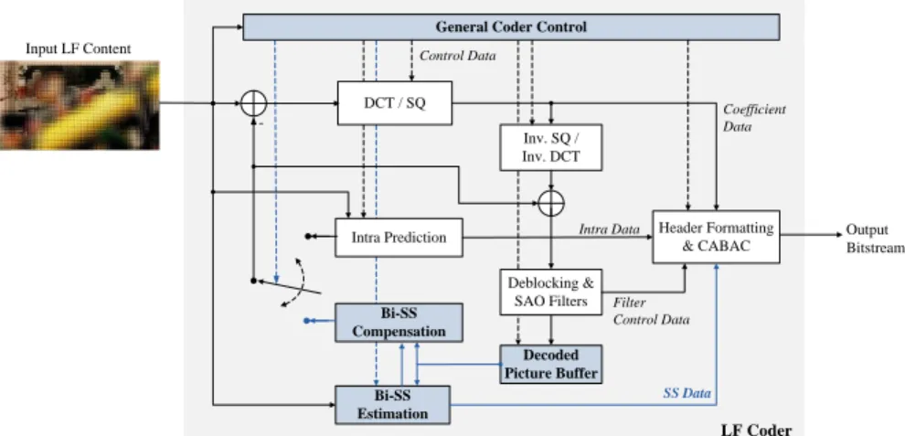
Fig. 1 presents the architecture of the proposed LFC Bi-SS solution, which is based on HEVC and comprises both additional and modified modules to efficiently handle LF content. Basically, the proposed codec introduces an additional type of prediction – the Bi-SS – and the encoder will choose the best, among Bi-SS and HEVC intra prediction, based on a conventional Rate-Distortion Optimization (RDO) process.

More specifically, enhancing the HEVC coding architecture with Bi-SS compensated prediction requires adaptations at the following stages of the coding process (as explained in the following): i) SS estimation; ii) prediction modes and block partitioning; iii) Bi-SS compensation; iv) Bi-SS vector prediction; and v) reference picture management.

2.1. Bi-SS Estimation

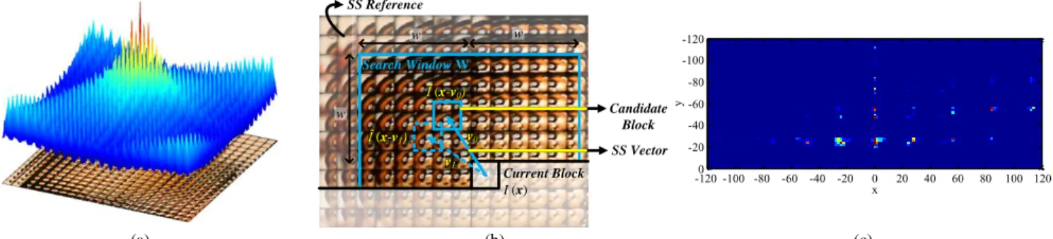
The Bi-SS estimation (depicted in Fig. 1) is used to exploit the cross-correlation existing in an MI neighborhood (see Fig. 2a) by estimating the prediction block with the highest similarity (according to appropriate criteria) to the current block in the previously coded and reconstructed area of the current picture itself (the SS reference, as seen in Fig. 2b). Hence, the relative position between the current and the ‘best’ candidate block is signaled by an SS vector, 𝒗0, (see Fig. 2b). Similarly to the

conventional HEVC inter P frame prediction, the best SS vector, 𝒗0𝑏𝑒𝑠𝑡, for the SS prediction can be found by minimizing the

Lagrangian cost function in (1) [35],

𝐽𝑈𝑛𝑖−𝑆𝑆= min_𝒗

0 ‖𝐼(𝒙) − 𝐼̃(𝒙 − 𝒗0)‖1+ 𝜆 𝑅(𝒗0) (1)

where 𝐼(𝒙) is a matrix variable representing the current block at position 𝒙 = (𝑥, 𝑦) in the LF image; Ĩ(𝒙 − 𝒗0) represents a

candidate block in the SS reference, Ĩ, with 𝒙 − 𝒗0∈ 𝐖 (see Fig. 2b); 𝑅(𝒗0) corresponds to an estimated number of bits for

encoding the SS vector 𝒗0 (i.e., the estimated number of bits necessary to encode the motion vector difference between 𝒗0 and

its predictor, selected as shown in Section 2.4); and 𝜆 is the Lagrangian multiplier. In addition, to keep the complexity low, the

l1-norm (or Sum of Absolute Differences (SAD)), ‖ ‖1, is used and a limited causal search window W is adopted. However, it

is worth noting that the search area shall be larger than the MI size to be able to exploit the inherent MI cross-correlations. Finally, the SS predictor block, 𝐼̂(𝒙), is derived as Ĩ(𝒙 − 𝒗0𝑏𝑒𝑠𝑡). As done in HEVC reference software version 14.0 [36], when

SAD is used as the distortion measure, 𝜆 is given by √𝜆𝐼𝑛𝑡𝑟𝑎, where 𝜆𝐼𝑛𝑡𝑟𝑎 is the Lagrangian multiplier computed for prediction

mode selection in intra-coded frames.

Notice that the SS estimation process in (1) only considers a single compensated signal for prediction of the current block, as previously proposed by the authors in [19], and for this reason will be hereinafter referred to as Uni-predicted Self-Similarity (Uni-SS) estimation. Moreover, further improvements to this estimation process will be proposed in Section 3 for allowing jointly estimated Bi-SS prediction.

2.2. Prediction Modes and Block Partitioning

The Bi-SS prediction is evaluated for all Coding Block (CB) sizes (i.e., from 64×64 down to 8×8) in the conventional RDO process to choose the best prediction mode. For this, the proposed Bi-SS method defines the following two additional prediction modes:

• Bi-SS mode – In this case, Bi-SS estimation (see Fig. 1) is used to find a prediction for encoding the current block. As in HEVC inter coding, the eight partition patterns, i.e., M×M, M×(M/2), (M/2)×M, (M/2)×(M/2), M×(M/4), M×(3M/4), (M/4)×M, and (3M/4)×M [37], are allowed to define a flexible way to partition the CB for the Bi-SS estimation process in Fig. 2b.

Fig. 1 Coding architecture of the proposed LFC Bi-SS solution based on HEVC (the novel and modified blocks are highlighted in blue). The HEVC blocks for motion estimation and compensation are here omitted since temporal prediction is not used in the proposed light field image coding solution.

DCT / SQ Inv. SQ / Inv. DCT Decoded Picture Buffer Input LF Content -Header Formatting & CABAC Control Data Intra Prediction

General Coder Control

Output Bitstream Deblocking & SAO Filters Coefficient Data Bi-SS Estimation Bi-SS Compensation SS Data Filter Control Data Intra Data LF Coder

• SS-skip mode – The SS-skip is employed only for the M×M partition pattern, and, in this case, the SS vector is directly derived from the Bi-SS vectors prediction presented Section 2.4, and no further information is transmitted.

2.3. Bi-SS Compensation

In this process (shown in Fig. 1), the inverse quantized and inverse transformed causal residual block is added to the prediction block to obtain the reconstructed block. The SS reference is then updated (for each CB) by including this reconstructed block as it will be available at the decoder side.

2.4. Bi-SS Vectors Prediction

In conventional video coding solutions, since neighboring motion vectors are likely to be correlated, they are usually predictively coded based on motion vectors of neighboring blocks. Regarding HEVC [23], this predictive coding of motion vectors was improved, relatively to previous video coding standards, by introducing a tool called Advanced Motion Vector Prediction (AMVP). Furthermore, an HEVC technique called merge mode is used to derive all motion data of a block (i.e., motion vectors and indices of the used reference pictures) from the neighboring blocks, replacing the direct and skip modes of the previous H.264/AVC standard. In these methods, a vector candidate (or merge candidate) list is built by selecting vectors from CBs in the spatial and temporal (co-located) neighborhood [37]. From these spatio-temporal candidates, the encoder selects the best predictor vector in an RDO sense, and transmits only the index of the chosen candidate in this list.

In addition to this, a set of new SS candidate vectors proposed in [19], referred to as MI-based vector prediction (MIVP) candidate vectors, is also included into AMVP and merge candidate lists to further improve the RD performance. As explained in [19], up to three MI-based candidate vectors (i.e., left, above, and above-left) are computed to force the candidate vectors to be distributed according to the structure of MIs. A detailed description of the MIVP candidate vectors selection is given in [19]. Regarding the proposed Bi-SS mode, if bi-prediction is used, two predictor vectors are derived from the AMVP method (one for each estimated SS vector) and the difference between the two SS estimated vectors and the corresponding predictor vectors are transmitted along with the indices of the chosen candidates in the list. In this case, the AMVP candidate list is constructed with the following candidates (for intra-coded frames):

• Spatial AMVP vector candidates – Up to two spatial vector candidates are derived from a set of five spatial neighboring CBs that were previously coded with Bi-SS mode. The position of these neighboring CBs are defined in HEVC standard [23].

• MI-based vector candidate – When less than two spatial vector candidates are available, one MI-based vector candidate is derived from the set of left, above, and above-left defined in MIVP.

• Zero vector candidates – Afterwards, zero vectors are added to fill, when necessary, the AMVP candidate list with up to two final candidates (as in HEVC [23]).

In the case of the SS-skip mode, bi-predicted merge candidates may be derived from the following merge candidate list: • Spatial merge vector candidates – Up to four spatial candidates from the set of five [23] neighboring CBs that were

coded with Bi-SS mode are included.

• MI-based vector candidates – The maximum size of the merge candidate list is signaled in the slice header syntax (being equal to five as defined by default in HEVC standard [23]). After selecting the spatial candidates, up to three MIVP merge candidates are included into the merge candidate list until the maximum number of candidates is reached.

(a) (b) (c)

Fig. 2 SS prediction: (a) inherent MI cross-correlation in a light field image neighborhood; (b) Bi-SS estimation process (example of a second candidate block and SS vector for bi-prediction is shown in dashed blue line); and (c) Heat map showing the SS vectors distribution when coding an LF image

Current Block I (x) Search Window W SS Vector Candidate Block v1 v0 Ĩ (x-v0) Ĩ (x-v1) SS Reference w w w x y -120 -100 -80 -60 -40 -20 0 20 40 60 80 100 120 -120 -100 -80 -60 -40 -20 0

• Additional merge candidates – Furthermore, if the merge candidate list is still not fully populated, bi-predicted candidates can also be derived by combining two existing candidates from different reference picture lists. When the list is still not full, zero motion candidates are included to complete the list.

An analysis of the influence of this MIVP scheme in the RD performance achieved by the Bi-SS prediction is presented in Section 3.5.

2.5. Reference Picture Management

To allow the Bi-SS estimation and Bi-SS compensation in intra-coded frames of HEVC, the reference lists construction and signaling need to be altered so as to include the SS reference. This process is similar to the temporal lists construction on HEVC inter-coded frames, and is managed by the general coder control block in Fig. 1 by using the concept of Reference Picture Set (RPS), which is signaled for each slice [37]. For this, the SS reference is made available at the decoded picture buffer (see Fig. 1) and marked to be used as a reference.

3. Proposed Jointly Estimated Bi-SS Compensated Prediction

To further improve the performance of the proposed Uni-SS LFC solution [19], a novel jointly estimated Bi-SS estimation and compensation scheme, which is based on the generic concept of superimposed prediction [33], is here proposed to replace the aforementioned Uni-SS estimation and compensation processes.

To motivate the adoption of this Bi-SS prediction in the LFC solution presented in Section 2, a theoretical analysis is firstly presented, which shows that other non-local spatial prediction schemes – such as the IntraBC [32], the preceding Uni-SS prediction presented in Section 2.1, and the solution for bi-prediction proposed in [20] – can be considered as restricted cases of the Bi-SS solution proposed here. Then, the Bi-SS candidate predictor estimation is proposed in Section 3.2 and the theoretical assumptions for its improved RD efficiency are experimentally analyzed in Sections 3.3 and 3.4, respectively, in terms the MI cross-correlation in LF images and in terms of the weighting factor used in the bi-prediction. Finally, the influence of the MIVP in the RD performance achieved for Bi-SS prediction is also analyzed in Section 3.5.

3.1. Theoretical Bi-SS Performance Analysis

The RD performance improvement due to the adoption of the jointly estimated Bi-SS prediction (presented in more detail in the following section) is based on three main hypotheses, which will be analyzed in this section:

1) With a large enough search window, 𝐖, (see Fig. 2b), it is possible to find two predictor blocks that properly represent the current block, 𝐼(𝒙), i.e., with low residual signal.

2) By combining two good predictor blocks, it is possible to further minimize the residual signal of the SS compensated prediction, compared to only using the uni-predicted SS candidate (as in the Uni-SS prediction [19] and in the IntraBC scheme [32]).

3) Jointly estimating the predictor blocks leads to better RD performance than deriving them independently (as in reference software for HEVC inter B frame coding [36] and in the bi-prediction solution proposed in [20]).

For this analysis, the performance of the proposed Bi-SS prediction is here modeled by the uncertainty [35] (or inaccuracy [33,38]) in the SS compensated prediction signal.

Regarding the first abovementioned hypothesis, it is valid due to the following facts:

• Given the small baseline between adjacent microlenses in the acquisition process, a significant cross-correlation exists between neighboring MIs, as shown by the autocorrelation function in Fig. 2a. It can be seen (Fig. 2a) that the autocorrelation function presents a regular structure of spikes and the constant distance between these regular spikes corresponds to the MI spacing in the array [19]. Since these highly-correlated samples are distributed along the MIs, it is likely that similarly good predictor blocks will be also distributed accordingly.

• It was shown in [19] that, when using the SS compensated prediction scheme for exploiting the inherent MI cross-correlation, the distribution of the chosen SS vectors is also related to the size and arrangement of the MIs in the MLA. This can be illustrated by the heat map in Fig. 2c, where brighter areas correspond to more frequent SS vector amplitudes. Hence, since these most frequent best uni-predicted SS vectors are distributed in all directions according to the MI arrangement, it is possible to consider that the second-best SS vector, which can also represent the current block properly, is likely to be found according to this distribution in a different direction.

Regarding the second and third hypotheses, the residual signal for the Bi-SS compensated prediction is given by (2), 𝑒(𝒙) = 𝐼(𝒙) − ∑ ℎ𝑝(𝒙) ∙ 𝐼̃(𝒙 − 𝒗𝑝)

1

𝑝=0 (2)

where 𝒙 − 𝒗𝑝∈ 𝑾, and ℎ𝑝 is the weight for each of these predictor blocks. For instance, for the bi-predicted SS candidate

predictor proposed in Section 3.2, ℎ𝑝= 1 2⁄ , ∀𝑝 ∈ {0,1}. However, as discussed in [35], the residual signal given by (2) can be

actually generalized as in (3) for 𝑁 predictor blocks.

𝑒(𝒙) = 𝐼(𝒙) − ∑ ℎ𝑝(𝒙) ∙ 𝐼̃(𝒙 − 𝒗𝑝) 𝑁−1

𝑝=0 (3)

The general case represented by (3) can also incorporate other types of candidate predictors reflecting the very flexible set of inter coding tools of HEVC [23]. In this case, 𝒉 = (ℎ0, ℎ1, … , ℎ𝑁−1) corresponds to a weight vector that is able to, for example,

incorporate [35]: i) the filtering used to generate the quarter-pixel interpolated signal in the SS estimation; and ii) the deblocking filter that can be applied in the SS reference. Each 𝐼̃𝑝(𝒙) = 𝐼̃(𝒙 − 𝒗𝑝) term can be interpreted as each of the

multiple compensated signals available for prediction of the current block. Hence, the uncertainty in a given Bi-SS compensated prediction can be modeled, as in [35], by an a posteriori probability density function, ℎ𝑝(𝒙), conditioned on the

encoded data. Therefore, since the expected value (the second term on the right-hand side of (3)) is the estimator that minimizes the mean-square error in the prediction of a random variable [35], it is possible to say that the residual signal in (3) can be minimized and, consequently, the accuracy of the prediction can be improved by using a larger set of multiple compensated signals and an optimized weight vector [35].

In addition, another possibility is to analyze the performance of the Bi-SS compensated prediction by modeling the inaccuracy of each used displacement vector 𝒗𝑝, as in [33,38]. For this, Fig. 2b shows that although the pixel correlation in the

raw LF image is not as smooth as in conventional 2D images, each MI itself has some degree of inter-pixel redundancy as in common 2D images (see Fig. 2b). Thus, it is possible to consider that samples inside each MI follow the same correlation model as samples in a 2D image (i.e., an isotropic exponentially decaying autocorrelation function). This assumption is reasonable at least for blocks 𝐼(𝒙) smaller than the MI resolution, and has been also adopted in [20,39] for LF images. With this assumption, the accuracy of the SS compensation can be measured by the displacement error variance [38], and the same signal model used in [33,38] can also be considered for the SS compensated prediction signal. In this case [33,38], 𝒉 denotes a row vector of impulse responses (ℎ0, ℎ1, … , ℎ𝑁−1) of a 2D prediction filter [38], and the residual signal is given by (4),

𝑒(𝒙) = 𝐼(𝒙) − 𝒉(𝒙) ∗ 𝑰̃(𝒙) (4)

where the second term on the right-hand side of the equation denotes a 2D convolution of the prediction filter 𝒉 with a column vector of 𝑁 multiple compensated signals 𝑰̃ = (𝐼̃0, 𝐼̃1, … , 𝐼̃𝑁−1)𝑇. In this model, both 𝐼 and each component of 𝑰̃ are assumed to

be wide sense stationary random processes with an additive Gaussian noise signal. Hence, these noisy signals may comprise all signal components of the SS compensated prediction that cannot be described by the translational displacement model [38].

Based on the abovementioned approximations, the conclusions from [33,38] also hold for validating the second and third hypotheses. Notably, with high rate assumptions:

• Concerning the second hypothesis, the optimal filter 𝒉 (i.e., that minimizes the mean square error) can be interpreted as a low pass filter that removes high frequency components from 𝑰̃ that are too noisy or that change too rapidly [38]. From the theoretical analysis in [38], it was concluded that increasing the number of equally good predictor blocks always led to bitrate savings compared to a more limited set of predictor blocks, even if the simple average filter is used, instead of considering an optimal filter 𝒉 in (4). Therefore, this suggests that increasing from one predictor block (in the previously proposed Uni-SS prediction [19]) to two predictor blocks (in the Bi-SS prediction proposed here) minimizes the residual signal in the SS compensated prediction.

• Concerning the third hypothesis, an extended analysis was performed in [33] for the case where the multiple compensated samples of 𝑰̃ are jointly estimated. In this case, the displacement error of all components of 𝑰̃ are assumed to be correlated, instead of being independent as assumed in [38]. Moreover, this analysis considered the simple average filtering case as for the proposed Bi-SS. Therefore, it was shown that a combination of two jointly estimated predictor blocks is more efficient than two independent predictor blocks [33]. Furthermore, it was concluded that, for jointly estimated predictors, the major portion of the gain is already achievable by only two predictor blocks [33]. This suggests that further RD gains can be achieved by jointly estimating the two predictor blocks for bi-prediction compared to

simply combining two best uni-predicted candidates (as in the HEVC reference software inter B frame coding [23] and in bi-predicted solution proposed in [20]).

Therefore, without loss of generality, the IntraBC scheme in [32], and the previously proposed LFC solutions in [19,20] can be seen as restricted cases of the Bi-SS solution being proposed here. In these cases [19,20,32], restrictions are imposed in the number of predictor blocks, the number of allowed partition patterns and sizes, and in the bi-prediction estimation process for each predictor block that is independently employed in different areas of the SS reference.

As it will be seen in Section 4, the theoretical insights from this section for the proposed Bi-SS solution are supported by the experimental results for LF images. Moreover, to extend the conclusions from this analysis, Section 3.4 also analyzes the RD performance for LF image coding when using different sets of weighting coefficients for Bi-SS prediction.

3.2. Bi-SS Candidate Predictors Estimation

Motivated by the theoretical analysis presented above, the proposed Bi-SS prediction is here presented, which is based on the generic concept of superimposed prediction [33].

More specifically, there is only a single reference picture available in the Bi-SS compensated prediction, i.e., the SS reference [18], and only two possible candidate predictors (instead of the three candidates of HEVC [23] that are used in [20]) are derived to predict the current block, namely: i) the Uni-SS candidate, and ii) the Bi-SS candidate.

The Uni-SS candidate predictor corresponds to the previously proposed SS prediction [19] (see Section 2.1), in which the predictor block is found by minimizing the Lagrangian cost function in (1).

The proposed Bi-SS candidate predictor differs from the HEVC reference software inter B frame bi-prediction, as well as from the bi-predicted solution in [20], for two main reasons:

1) The two predictor blocks in the Bi-SS solution are derived from the same reference picture (the SS reference) and are estimated in the same search window, 𝐖 (see Fig. 2b). Consequently, they can be located in the same MI (different to [20]) and in overlapped pixel positions (as illustrated by the dashed blue lines in Fig. 2b).

2) To further improve the prediction efficiency, these two predictor blocks are jointly estimated in the complete search window (as explained below), instead of combining two best uni-predicted candidates (as in [20]).

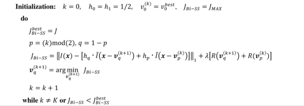
For jointly estimating the two predictor blocks, the locally optimal rate-constrained algorithm proposed in [34] (see Fig. 3) is used. This algorithm avoids searching through all possible combinations of two candidate predictor blocks 𝐼̃(𝒙 − 𝒗0) and

𝐼̃(𝒙 − 𝒗1) inside 𝐖. For this, in each algorithm iteration, 𝑘, an optimal SS candidate vector 𝒗𝑞(𝑘+1) (with index 𝑞 ∈ {0,1}) is

found by minimizing the Lagrangian cost function conditioned to the optimal SS candidate vector found in the previous iteration 𝒗𝑝(𝑘) (with 𝑝 ∈ {0,1}). Therefore, the algorithm is focused on finding an optimized vector 𝒗1 conditioned to a known

vector 𝒗0 in even iterations, and vice versa in odd iterations. For instance, in the first iteration, 𝑘 = 0, 𝑝 = 0, 𝑞 = 1, and the

optimal 𝒗1(1) is found by fixing 𝒗0(0)= 𝒗0𝑏𝑒𝑠𝑡 (the best uni-predicted SS candidate vector). Similarly, in the second iteration, 𝑘 =

1, 𝑝 = 1, 𝑞 = 0, and the optimal 𝒗0(2) is found by fixing 𝒗1(1) (which was found in the previous iteration). Similarly to (1), the

Lagrangian cost function show in Fig. 3 is used to find the optimal SS vector in each iteration, where 𝜆 is computed as √𝜆𝐼𝑛𝑡𝑟𝑎

[36] and 𝑅(𝒗𝑞(𝑘+1)) + 𝑅(𝒗𝑝(𝑘)) corresponds to the estimated number of bits for encoding the SS vectors 𝒗0 and 𝒗1 given in each

Initialization: 𝑘 = 0, ℎ0= ℎ1= 1/2, 𝑣0(𝑘)= 𝑣0𝑏𝑒𝑠𝑡, 𝐽𝐵𝑖−𝑆𝑆= 𝐽𝑀𝐴𝑋 do 𝐽𝐵𝑖−𝑆𝑆𝑏𝑒𝑠𝑡 = 𝐽 𝑝 = (𝑘)mod(2), 𝑞 = 1 − 𝑝 𝐽𝐵𝑖−𝑆𝑆= ‖𝐼(𝒙) − [ℎ𝑞∙𝐼̃(𝒙 − 𝒗𝑞(𝑘+1)) + ℎ𝑝∙𝐼̃(𝒙 − 𝒗𝑝(𝑘))]‖₁+ 𝜆[𝑅(𝒗𝑞(𝑘+1)) + 𝑅(𝒗𝑝(𝑘))] 𝒗_𝑞(𝑘+1)_{= arg min} 𝒗𝑞(𝑘+1) 𝐽_{𝐵𝑖−𝑆𝑆} 𝑘 = 𝑘 + 1 while 𝑘 ≠ 𝐾 or 𝐽𝐵𝑖−𝑆𝑆< 𝐽𝐵𝑖−𝑆𝑆𝑏𝑒𝑠𝑡

Fig. 3 Algorithm for jointly estimating the two predictor blocks 𝐼̃(𝒙 − 𝒗0) and 𝐼̃(𝒙 − 𝒗1) for the proposed Bi-SS candidate predictor. The index 𝑞 defines

iteration, i.e., the estimated number of bits necessary to encode the motion vector difference between the SS vectors and their predictor vectors and for signaling the vector predictor using AMVP.

The maximum number of iterations, 𝐾, defines a tradeoff between complexity and RD performance and can be adjusted according to the system constraints. In this work, 𝐾 = 2 and, consequently, the corresponding complexity is similar to that of HEVC inter B-frame with one active reference in each reference picture list.

Finally, the best prediction between Uni-SS and Bi-SS candidates is also chosen in terms of conventional RDO [35] by comparing the associated Lagrangian costs 𝐽𝑈𝑛𝑖−𝑆𝑆𝑏𝑒𝑠𝑡 and 𝐽𝐵𝑖−𝑆𝑆𝑏𝑒𝑠𝑡 , respectively found in (1) and Fig. 3.

3.3. Bi-SS Prediction Analysis for Different MI Cross-Correlation

This section aims at analyzing how close the theoretical conclusions drawn in [33,38] and the approximations considered in Section 3.1 are to the experimental results when using the proposed Bi-SS prediction for LF image coding. More specifically, this analysis focuses on the influence of the MI cross-correlation, inherently present in LF images, in the performance of the Bi-SS prediction proposed in Section 3.2. For this, Tables 1 and 2 summarize some statistics of relevant results when encoding different LF test images (see Section 4), such as: percentages of prediction mode usage, SS bi-prediction usage, and coding block size (CBS) usage. These statistics are shown for higher bitrates in Table 1 (corresponding to quantization parameter value 22) and for lower bitrates in Table 2 (corresponding to quantization parameter value 42). In addition, some RD results comparing Uni-SS and Bi-SS prediction are presented using the Bjøntegaard delta (BD) [42] metrics, i.e., in terms of the luma PSNR of the LF image and the corresponding bitrate (BR) in terms of bits per pixel (bpp) for four different Quantization Parameter (QP) values. In this case, the sets of QP values {22, 27, 32, 37} and {27, 32, 37, 42} were considered for analyzing the performance, respectively, for high and low bitrates.

For better analyzing these results, two different situations where the MI cross-correlation is differently distributed in a

neighborhood are considered (corresponding to the highlighted values in Tables 1 and 2). For the first situation, a second frame

Table 2 Influence of MI cross-correlation in mode selection statistics and RD performance for low bitrate

Image Prediction Modes Statistics SS Prediction Statistics CBS Statistics

LFC Bi-SS vs. LFC Uni-SS

Intra SS SS-skip Uni-Prediction Bi-Prediction 64×64 32×32 16×16 8×8 BD-PSNR BD-BR

Plane and Toy (frame 123) 30.5 % 46.2 % 23.3 % 87.1 % 12.9 % 0.1% 3.9 % 22.3 % 73.7 % 0.3 dB -4.9 %

Plane and Toy (frame 23) 43.7 % 30.5 % 25.8 % 75.0 % 25.0 % 0.6 % 14.9 % 32.4 % 52.1 % 0.4 dB -6.5 %

Demichelis Spark 18.2 % 46.1 % 35.7 % 61.1 % 38.9 % 8.5 % 40.0 % 33.0 % 18.5 % 0.7 dB -17.3 % Laura 22.5 % 45.1 % 32.4 % 74.1 % 25.9 % 0.1 % 11.0 % 36.0 % 52.9 % 0.5 dB -9.5 % Jeff 21.0 % 38.7 % 40.3 % 76.8 % 23.2 % 1.1 % 18.5 % 40.5 % 39.9 % 0.4 dB -8.8 % Seagull 15.9 % 36.5 % 47.6 % 81.0 % 19.0 % 0.7 % 20.5 % 39.6 % 39.2 % 0.6 dB -13.8 % Zhengyun1 22.0 % 34.8 % 43.3 % 78.4 % 21.6 % 0.9 % 19.7 % 42.7 % 36.6 % 0.4 dB -9.1 % Flowers 75.7 % 18.7 % 5.5 % 62.5 % 37.5 % 12.3 % 43.9 % 17.0 % 26.8 % 0.1 dB -3.4 % Vespa 47.0 % 29.4 % 23.6 % 41.1 % 58.9 % 31.6 % 40.8 % 15.1 % 12.5 % 0.5 dB -20.6 % Ankylosaurus_&_Diplodocus_1 45.7 % 16.6 % 37.8 % 59.8 % 40.2 % 51.5 % 30.5 % 10.8 % 7.1 % 0.5 dB -33.6 % Fountain_&_Vincent_2 40.7 % 40.4 % 18.9 % 40.7 % 59.3 % 17.8 % 39.9 % 18.5 % 23.7 % 0.6 dB -16.4 % Color_Chart_1 26.4 % 33.6 % 40.0 % 26.1 % 73.9 % 40.7 % 33.9 % 13.6 % 11.8 % 0.3 dB -15.0 % ISO_Chart_12 46.9 % 31.5 % 21.6 % 40.2 % 59.8 % 25.2 % 45.3 % 21.2 % 8.3 % 0.6 dB -20.8 %

Table 1 Influence of MI cross-correlation in mode selection statistics and RD performance for high bitrate

Image Prediction Modes Statistics SS Prediction Statistics CBS Statistics

LFC Bi-SS vs. LFC Uni-SS

Intra SS SS-skip Uni-Prediction Bi-Prediction 64×64 32×32 16×16 8×8 BD-PSNR BD-BR

Plane and Toy (frame 123) 57.2 % 42.3 % 0.5 % 60.4 % 39.6 % 0.0 % 0.9 % 9.3 % 89.8 % 0.3 dB -4.5 %

Plane and Toy (frame 23) 67.8 % 30.9 % 1.3 % 54.2 % 45.8 % 0.0 % 3.0 % 11.4 % 85.6 % 0.4 dB -6.1 %

Demichelis Spark 53.3 % 39.9 % 6.9 % 48.8 % 51.2% 0.1% 3.8 % 18.2 % 77.9 % 0.5 dB -14.9 % Laura 36.3 % 62.9 % 0.7 % 44.9 % 55.1 % 0.0 % 1.1 % 20.7 % 78.3 % 0.5 dB -8.6 % Jeff 39.6 % 58.6 % 1.7 % 44.5 % 55.5 % 0.0 % 4.5 % 27.6 % 67.9 % 0.5 dB -10.4 % Seagull 27.3 % 66.3 % 6.4 % 47.3 % 52.7 % 0.0 % 3.2 % 29.8 % 67.0 % 0.7 dB -14.4 % Zhengyun1 58.3 % 40.7 % 1.0 % 47.5 % 52.5 % 0.0 % 3.3 % 20.8 % 76.0 % 0.4 dB -9.9 % Flowers 72.7 % 26.5 % 0.8 % 45.3 % 54.7 % 0.8 % 15.3 % 15.8 % 68.1 % 0.1 dB -3.1 % Vespa 29.9 % 65.6 % 4.5 % 26.7 % 73.3 % 0.4 % 7.9 % 27.7 % 64.0 % 0.5 dB -18.9 % Ankylosaurus_&_Diplodocus_1 14.7 % 84.6 % 0.7 % 10.8 % 89.2 % 0.2 % 3.5 % 30.0 % 66.4 % 0.7 dB -44.1 % Fountain_&_Vincent_2 40.9 % 57.4 % 1.7 % 16.3 % 83.7 % 0.6 % 12.3 % 23.1 % 64.0 % 0.7 dB -16.6 % Color_Chart_1 20.3 % 75.4 % 4.3 % 16.2 % 83.8 % 0.1 % 2.5 % 28.4 % 69.0 % 0.4 dB -22.5 % ISO_Chart_12 23.5 % 73.7 % 2.8 % 21.3 % 78.7 % 0.1 % 5.1 % 28.3 % 66.5 % 0.6 dB -22.7 %

of Plane and Toy sequence (frame 23) is used to exemplify the case where the MI cross-correlation varies for the same camera parameters due to the different distance of the main object relatively to the camera [40]. In this case, Plane and Toy (frame 23) presents a more rapid decrease in the MI cross-correlation in a neighborhood when compared to Plane and Toy (frame 123). For the second situation, two raw LF images, Jeff and ISO_Chart_12, with considerably larger and smaller MI resolutions, respectively, are used to illustrate the case in which the MI cross-correlation varies due to a change in the camera parameters. In this case, the aperture of the microlens (which usually corresponds to the size of the MI) limits its field of view [41], and consequently, the smaller the MI is, the less correlated it will be with MIs in its neighborhood (i.e., less overlapped areas of the scene will be captured by neighbor MIs). For completeness, Tables 1 and 2 also show statistics for all LF test images.

The results in Table 1 illustrate the influence of the MI cross-correlation in the usage and performance of the proposed Bi-SS approach for higher bitrates. Comparing the results for Plane and Toy (frame 123) and Plane and Toy (frame 23), it can be seen that the percentage of SS bi-prediction is larger in the case where the MI cross-correlation decreases rapidly (frame 23). Moreover, the bi-prediction is also able to achieve larger bit savings in this case (frame 23) when compared to the LFC Uni-SS solution, where only uni-prediction is used. Somehow similar to the abovementioned conclusion, the usage percentage of bi-prediction tends to be also considerably larger for the case of ISO_Chart_12 where the MI cross-correlation is smaller due to changes in the camera parameters (compared to Jeff).

In addition, Fig. 4 illustrates the Bi-SS vectors distribution for the LF images Plane and Toy (frame 23) and ISO_Chart_12. It can be seen that the Bi-SS vectors are also distributed according to MI structure of each tested LF image (as was also concluded for the uni-predicted SS vectors [19]). This is evident for ISO_Chart_12 (in Fig. 4b) where the MIs in the raw LF image are distributed according to a hexagonal grid, and, consequently, the SS vectors distribution (Fig. 4b) follow the same structure. This fact supports the assumptions made in Section 3.1 that more than one good predictor is likely to be found in all directions, distributed according to the MI size and arrangement in the array. Moreover, analyzing the distribution of these SS vectors along the raw LF image (rightmost images in Fig. 4), it can be seen that, although the amplitude of the SS vectors respects the MI structure, the direction tends to be dictated by the object boundaries and textures.

It is also worthwhile to notice (Table 1) that, for all tested LF images considered in Section 4, most of the coding blocks tend to be partitioned down to 8×8 blocks, being smaller than the MI resolution. These results support the assumptions used in the theoretical analysis from Section 3.1, which considered that samples inside each MI follow the same correlation model as samples in a 2D image.

To complete this analysis, Table 2 illustrates the statistical results also for lower bitrates, so as to analyze the performance of the Bi-SS prediction when the SS reference degrades. Comparing the results in Tables 1 and 2 for all test images, it can be observed that using higher QP values results in increasing percentages of usage of the SS uni-prediction, as well as SS-skip modes. This is due to the fact that the Lagrangian multiplier, in (1) and Fig. 3, increases with increasing QP values [35] and, for this reason, the possible quality improvements of using the bi-prediction do not justify the higher number of bits needed for transmitting the SS vectors when minimizing the Lagrangian cost.

(a)

(b)

Fig. 4 Bi-predicted SS vector distribution (from left to right): heat map of SS vector distribution for first candidate predictor, heat map of SS vector distribution for second candidate predictor, distribution of first (in blue) and second (in red) SS vectors along the encoded raw image. Results are illustrated for: (a) Plane and Toy (frame 23); and (b) ISO_Chart_12.

-120 -100 -80 -60 -40 -20 0 20 40 60 80 100 120 -120 -100 -80 -60 -40 -20 0 x y -120 -100 -80 -60 -40 -20 0 20 40 60 80 100 120 -120 -100 -80 -60 -40 -20 0 x y -120 -100 -80 -60 -40 -20 0 20 40 60 80 100 120 -120 -100 -80 -60 -40 -20 0 x y -120 -100 -80 -60 -40 -20 0 20 40 60 80 100 120 -120 -100 -80 -60 -40 -20 0 x y

3.4. Bi-SS Prediction Analysis for Different Weighting Coefficients

This section aims at analyzing the RD performance of the proposed LFC Bi-SS solution when different sets of weighting coefficients, ℎ0 and ℎ1 (see Fig. 3), are used for Bi-SS prediction.

For this, the HEVC weighted prediction signaling [37] is used. Basically, the usage of explicit weighted prediction in HEVC is activated by a flag in the Picture Parameter Set (PPS), and different integer weighting factors, 𝑤𝑝, and offset values, 𝑜𝑝, can

be assigned for prediction in each slice [37]. The resulting predictor block 𝐼̂(𝒙) for weighted bi-prediction can be then derived by [37]:

𝐼̂(𝒙) = ⌊𝑤0∙ 𝐼̃(𝒙 − 𝒗0) + 𝑤1∙ 𝐼̃(𝒙 − 𝒗1) + (𝑜0+ 𝑜1+ 1) ∙ 2

𝐿𝑊𝐷

2 ∙ 2𝐿𝑊𝐷 ⌋ (5)

where 𝐿𝑊𝐷 is a log weight denominator rounding factor [37] used to normalize the integer weighting factors and the sub-sample interpolation filtering process [43]. Notice that determining suitable weighting factors and offsets is out of the scope of HEVC standard and they are directly derived from the bitstream at the decoder side.

In this case, the following three LFC Bi-SS solutions are here tested and compared:

1) LFC Bi-SS (ℎ0= ℎ1= 1/2) – This corresponds to the proposed Bi-SS prediction, where the average weighting

coefficients are used. In (5), this corresponds to having 𝑤0= 𝑤1= 1, 𝐿𝑊𝐷 = 0, and 𝑜0= 𝑜1= 0.

2) LFC Bi-SS (ℎ0= 1/4 , 𝑎𝑛𝑑 ℎ1= 3/4) – In this case, weighted Bi-SS prediction is used, where the average weighting

coefficients in Fig. 3 are replaced by ℎ₀= 1/4 and ℎ₁= 3/4. In (5), this corresponds to having 𝑤₀= 1, 𝑤₁= 3, 𝐿𝑊𝐷 = 1, and 𝑜0= 𝑜1= 0.

3) LFC Bi-SS (ℎ0= 1/8 , 𝑎𝑛𝑑 ℎ1= 7/8) – In this case, weighted Bi-SS prediction is used with weighting coefficients

ℎ0= 1/8 and ℎ1= 7/8. In (5), this corresponds to having 𝑤0= 1, 𝑤1= 7, 𝐿𝑊𝐷 = 2, and 𝑜0= 𝑜1= 0.

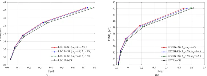
Due to space limits, Fig. 5 illustrates the results for only two LF images (i.e., Seagull and Vespa), but the conclusions are consistent for all LF test images considered in Section 4. From these results, it can be seen that the LFC Bi-SS solution using the average weighting coefficients always presents the best RD performance. Moreover, the less asymmetric the weighting coefficients are, the better the RD efficiency of the LFC Bi-SS solution is shown to be. In addition, in all cases, the weighted Bi-SS always outperform the LFC Uni-SS solution. For this reason, the average weighting coefficients are here considered to the proposed LFC Bi-SS solution.

Notice that it was not under the scope of this work to develop an optimized set of weighting coefficients for each CB (instead of fixing it for each slice). In fact, the theoretical analysis in [38] suggested that it is still possible to achieve further RD performance improvements by adaptively estimating these weighting coefficients; this will be considered in future work, as well as the experimental validation, for LF image coding, of the theoretical assumption made in [33] that suggests that the major portion of the gain is already achievable by only two predictor blocks.

(a) (b)

Fig. 5 RD performance of the proposed LFC Bi-SS solution (compared to the LFC Uni-SS solution) with different sets of weighting coefficients (QP values 22, 27, 32, 37, and 42). The results are show for two LF test images: (a) Seagull, and (b) Vespa

3.5. MIVP Efficiency Analysis for Bi-SS Prediction

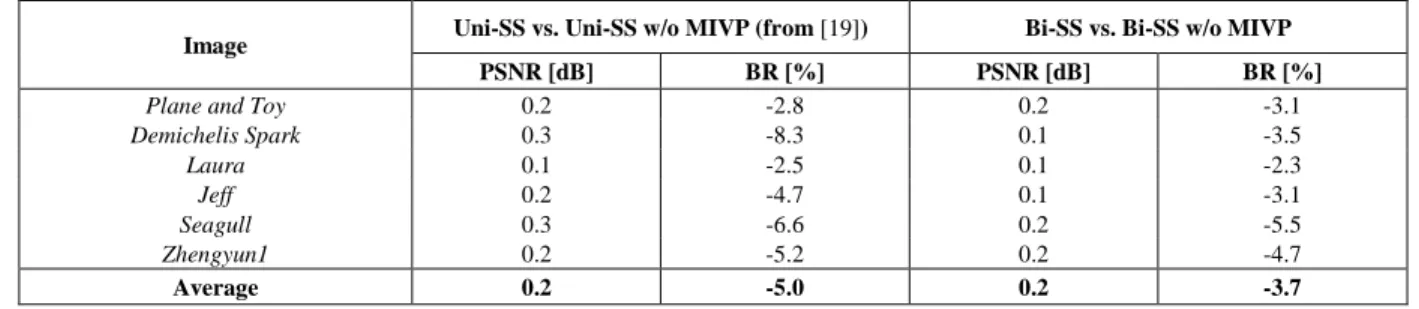
To separately analyze the RD efficiency of using the MIVP vector prediction for Bi-SS prediction, Table 3 shows some preliminary results for comparing the performance of Bi-SS prediction with MIVP (referred to as Bi-SS w/ MIVP) and without MIVP (referred to as Bi-SS w/o MIVP). These results are then compared to the achieved RD improvements presented for the previously proposed LFC Uni-SS solution in [19] (i.e., Uni-SS solution with and without MIVP).

In these tests, the same test conditions adopted in [19] are here used. Notably, HEVC reference software version 14.0 [36] is used as the benchmark, as well as the base software for implementing the proposed codec. RD performance is evaluated here for six different LF images through the BD [42] metrics, i.e., in terms of the luma PSNR of the LF image and the corresponding bitrate (BR) in terms of bits per pixel (bpp) for four QP values (27, 32, 37, and 42). These results of the MIVP influence on RD performance for Uni-SS prediction can also be found in [19].

From these results, it is possible to see that the gains of including the MIVP candidate vectors for Bi-SS prediction are slightly lower than for Uni-SS prediction. However, the MIVP is still relevant for the LFC Bi-SS solution, leading to further bit savings of up to 5.5% (for LF test image Seagull).

4. Performance Evaluation

This section assesses the performance of the complete LFC Bi-SS codec. For this, the test conditions are firstly introduced and, then, the obtained results are presented and discussed.

4.1. Test Conditions

The test conditions to evaluate the performance of the proposed LFC Bi-SS solution can be summarized as follows.

4.1.1. Test Images

Twelve LF test images with different camera setups and scene characteristics are used (see Fig. 6 and Table 4) so as to achieve representative RD results. These are: Plane and Toy (frame number 123 of the sequence with same name) and

Demichelis Spark [44] (first frame of a video sequence with same name); Laura, Fredo, Seagull, and Zhengyun [45]; and Flowers, Vespa, Ankylosaurus_&_Diplodocus_1, Fountain_&_Vincent_2, Color_Chart_1, and ISO_Chart_12 [46].

The (raw) LF test images were converted to the Y’CbCr 4:2:0 color format before being encoded.

4.1.2. Coding Conditions

The experimental results that are presented in this section considered the following test conditions:

1) Codec Software Implementation – The reference software of HEVC version 14.0 [36] was used as the benchmark, as well as the base software for implementing the proposed codec.

2) Search Range – A search range value of 128 was adopted for all tested LF images (i.e., w=128 in Fig. 2b).

3) Search Strategy – The full search algorithm with the HEVC quarter-pixel accuracy was used since fast search algorithms proposed for 2D video coding and for SCC have shown to present significant drop in RD performance for LF image coding [20].

4) Coding Configuration – The results are presented using the Main Still Picture profile [23] and five QP values are considered, i.e.: 22, 27, 32, 37, and 42.

Table 3. RD performance for LFC Bi-SS solution using MIVP (for QP values 27, 32, 37, and 42)

Image Uni-SS vs. Uni-SS w/o MIVP (from [19]) Bi-SS vs. Bi-SS w/o MIVP

PSNR [dB] BR [%] PSNR [dB] BR [%]

Plane and Toy 0.2 -2.8 0.2 -3.1

Demichelis Spark 0.3 -8.3 0.1 -3.5 Laura 0.1 -2.5 0.1 -2.3 Jeff 0.2 -4.7 0.1 -3.1 Seagull 0.3 -6.6 0.2 -5.5 Zhengyun1 0.2 -5.2 0.2 -4.7 Average 0.2 -5.0 0.2 -3.7

5) RD Evaluation – The RD performance was evaluated in terms of three different objective quality metrics: i) Overall PSNR; ii) Rendering-dependent PSNR (PSNR5×5Views); and iii) Rendering-dependent SSIM (SSIM5×5Views). The overall

PSNR is calculated by taking the luma PSNR of the raw LF image. Differently, the rendering-dependent metrics (PSNR5×5Views and SSIM5×5Views) are measured in terms of the average luma PSNR and SSIM calculated for a set of

views rendered from the reconstructed LF content, similarly to the metrics proposed in [6]. To have a representative number of rendered views, a set of 5×5 views was rendered from equally distributed directional positions. For rendering the views from LF images captured using a focused LF camera setup (Table 4), the algorithm proposed in [47] and referred to as Basic Rendering algorithm was used. In this case, the plane of focus was chosen to represent the case where the main object of the scene is in focus. For LF images captured using the traditional LF camera setup (Table 4), 5×5 VIs were extracted. The rate is given in terms of bpp value, which is calculated with the number of bits needed for encoding the LF image divided by its corresponding number of pixels given in Table 4 (bpp).

4.1.3. Benchmark Solutions

In order to assess the RD performance for different local and non-local spatial prediction schemes, five HEVC-based coding solutions are compared against the proposed LFC Bi-SS. To guarantee a fair comparison between all of them, the same test conditions presented in Section 4.1.2 are also adopted. These five benchmark solutions are:

(a) (b) (c) (d)

(e) (f) (g) (h)

(i) (j) (k) (l)

Fig. 6 Central rendered view from each test LF image: (a) Plane and Toy, (b) Demichelis Spark; (c) Laura, (d) Jeff, (e) Seagull, (f) Zhengyun1, (g) Flowers, (h) Vespa, (i) Ankylosaurus_&_Diplodocus_1, (j) Fountain_&_Vincent_2, (k) Color_Chart_1, and (l) ISO_Chart_12

Table 4. Description of LF test images in Fig. 6

Image Resolution LF camera setup MLA structure MI Resolution

Plane and Toy 1920×1088 Focused LF camera (Plenoptic camera 2.0) Rectangular grid of squared MIs 28×28* Demichelis Spark 2880×1620 Focused LF camera (Plenoptic Camera 2.0) Rectangular grid of circular MIs 38×38* Laura 7240 ×5232 Focused LF camera (Plenoptic Camera 2.0) Rectangular grid of squared MIs 74×74* Jeff 7240 ×5232 Focused LF camera (Plenoptic Camera 2.0) Rectangular grid of squared MIs 74×74* Seagull 7240 ×5232 Focused LF camera (Plenoptic Camera 2.0) Rectangular grid of squared MIs 74×74* Zhengyun1 7240 ×5232 Focused LF camera (Plenoptic Camera 2.0) Rectangular grid of squared MIs 74×74* Flowers 7728×5368 Traditional LF camera (Plenoptic Camera 1.0) Hexagonal grid of circular MIs 15×15* Vespa 7728×5368 Traditional LF camera (Plenoptic Camera 1.0) Hexagonal grid of circular MIs 15×15* Ankylosaurus_&_Diplodocus_1 7728×5368 Traditional LF camera (Plenoptic Camera 1.0) Hexagonal grid of circular MIs 15×15* Fountain_&_Vincent_2 7728×5368 Traditional LF camera (Plenoptic Camera 1.0) Hexagonal grid of circular MIs 15×15* Color_Chart_1 7728×5368 Traditional LF camera (Plenoptic Camera 1.0) Hexagonal grid of circular MIs 15×15* ISO_Chart_12 7728×5368 Traditional LF camera (Plenoptic Camera 1.0) Hexagonal grid of circular MIs 15×15*

1) HEVC – In this case, the original LF image is encoded with HEVC [36], using the Main Still Picture profile [23]. 2) HEVC SCC – In this case, the original LF image is encoded using the HEVC SCC reference software version 1.0 [48],

where IntraBC prediction [32] is used. As previously discussed in this paper, this solution is a restricted case of the proposed LFC Bi-SS since a reduced set of coding options is used, such as: i) only uni-prediction estimation is allowed considering only integer-pixel precision; ii) partition patterns are limited (i.e., M×M, M×(M/2), (M/2)×M, and (M/2)×(M/2) ); iii) CB sizes are also limited (CBs larger than 16×16 are skipped based on a threshold on the RD cost); and iv) only one dimensional (1D) vectors for 16×16 CBs are allowed. However, it is worth mentioning that some improvements for the IntraBC prediction have been continuously included. For instance, in the HEVC SCC reference software 1.0, the search window was expanded over the entire CB row or column (for 16×16 CBs), and over some positions in the entire picture by using a hash-based search (for 8×8 CBs).

3) LFC Uni-SS – In this case, the original LF image is encoded with the authors’ previous solution proposed in [19], where only the uni-predicted candidate is available for the SS estimation and compensation. This solution also uses the MIVP candidate vectors for improving the coding performance (as in the proposed LFC Bi-SS). A search area with w=128 (in Fig. 2b) is also adopted in this case.

4) LFC Restricted-SS – In this case, the original LF image is encoded with the author’s implementation of the solution proposed in [20], where bi-prediction is also allowed by simply using the HEVC inter B-frame prediction. For this, and as explained in [20], the SS reference search area is separated into two different parts, which are assumed to be two different reference pictures [20]. Therefore, as in HEVC inter B-frame prediction, three candidate predictors can be derived: the two best (uni-predicted) candidates from each of the two reference pictures, and a linear combination of them for bi-prediction. As discussed in Section 3, this solution can be seen as a restricted case of the Bi-SS prediction proposed here. It is also worthwhile to notice that, the solution presented in [20] (as well as the author’s implementation of this solution) does not include the MIVP candidate vectors that are used in both LFC Uni-SS and LFC Bi-SS solutions. A search area with w=128 (in Fig. 2b) is also adopted in this case.

5) LFC GPR – In this case, an HEVC-based LFC solution using the implicit GPR-based prediction method proposed in [22] is considered. Different from the SS prediction, the predictor block is here given as a linear combination of six nearest neighbor patches, which are implicitly found in two different search windows: i) horizontal search window (defined as the causal area in the same CB row): ii) the vertical search window (defined as the causal area in the same CB column). Afterwards, the set of weighting coefficients for combining these six patches is implicitly determined by solving a GPR and the same process to find the nearest neighbor patches and weighting coefficients is replicated at the decoder side to derive the prediction. For this comparison, the results presented in [22] for coding using this LFC GPR solution are compared to the results for the proposed LFC Bi-SS solution considering the same test conditions (described in [22]). Notably, the results are shown using the BD metrics in terms of the overall PSNR with respect to HEVC reference software [36] with “Intra, main” configuration and considering four different QP values: 22, 27, 32, and 37 (as in [22]).

It is important to notice that, other benchmark solutions have already been compared against the authors’ previous solution LFC Uni-SS in [19], (e.g., a multiview-based method, similar to the proposed in [12,13]). For a more complete performance comparison, please also refer to [19].

4.2. Overall RD Performance

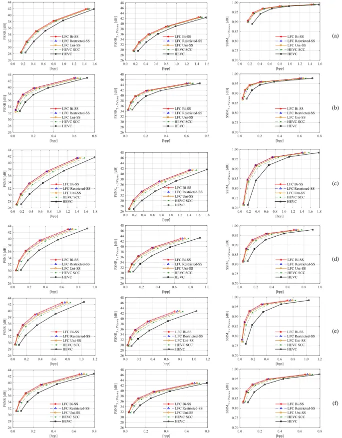
Figs. 7 and 8 illustrate the RD performance of the proposed LFC Bi-SS using three different objective quality metrics, i.e., the overall PSNR, and the rendering-dependent metrics PSNR5×5Views and SSIM5×5Views. Additionally, Tables 5 and 6 present the

LFC Bi-SS RD performance against four benchmark solutions (i.e., HEVC, HEVC SCC, LFC Uni-SS, and LFC Restricted-SS) in terms of BD metrics, respectively, for higher and lower bpp values. It is worth noting that the comparison between the proposed LFC Bi-SS and the LFC GPR solutions will be separately performed in Section 4.4 since, in this case, the results presented in [22] for the LFC GPR solution is directly compared to the LFC Bi-SS solution RD results when using the same set of LF images as well as the same test coding conditions adopted in [22].

(a) (b) (c) (d) (e) (f)

Fig. 7 RD performance (QP values 22, 27, 32, 37, and 42) for the LF test images: (a) Plane and Toy, (b) Demichelis Spark; (c) Laura, (d) Jeff, (e) Seagull, and (f) Zhengyun1

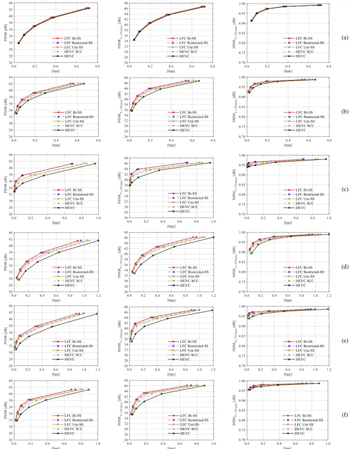
(a) (b) (c) (d) (e) (f)

Fig. 8 RD performance (QP values 22, 27, 32, 37, and 42) for the LF test images: (a) Flowers, (b) Vespa, (c) Ankylosaurus_&_Diplodocus_1, (d) Fountain_&_Vincent_2, (e) Color_Chart_1, and (f) ISO_Chart_12

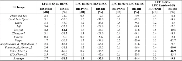
As can be observed in Figs. 7 and 8, independently of the adopted objective quality metrics, the results follow the same trend and the proposed LFC Bi-SS solution outperforms the other benchmark solutions in all cases. Moreover, as shown in Tables 5 and 6, significant gains can be achieved by the proposed LFC Bi-SS solution mainly for lower bpp values (Table 6), achieving in average 2.7 dB (or 51.5 % of bit savings) against HEVC, 1.3 dB (or 32.0 % of bit savings) against HEVC SCC, 0.5 dB (or 14.4 % of bit savings) against LFC Uni-SS, and 0.3 dB (or 9.4 % of bit savings) against LFC Restricted-SS. Additionally, as hypothesized in the theoretical analysis of Section 3.1, increasing the number of predictor blocks from the LFC Uni-SS solution to the LFC Bi-SS solution led to bit savings of up to 22.7 % (Table 5). Furthermore, comparing to the LFC Restricted-SS solution, it can be seen that by jointly estimating both candidate predictors, instead of devising them separately from different areas, further bit savings of up to 16.9 % (Table 6) can be achieved.

Moreover, comparing the achieved performance gains due to MIVP (Table 3) with the results against the LFC Uni-SS in Table 5, it can be seen that most of the LFC Bi-SS performance gains come from the usage of an improved bi-prediction scheme. However, it should be noticed that the MIVP is mainly advantageous for improving the performance against the LFC Restricted-SS (see Table 5), even when only Uni-SS prediction is allowed. For instance, for the LF image Plane and Toy, the LFC Uni-SS solution (using the MIVP) presents a slightly better performance than the LFC Restricted-SS solution (where the MIVP is not used).

Regarding the performance for different LF image characteristics, it was observed that the coding efficiency of the SS compensated prediction is not as good for close-up images. This can be seen by analyzing the results for LF image Flowers (close-up image) against Fountain_&_Vincent_2 (see Fig. 6g and j, respectively), but it was also observed for other LF images of the dataset in [46]. In these close-up images, most of the coding blocks (about 75 % of them) are coded using HEVC intra prediction.

Table 6. LFC Bi-SS overall RD performance with respect to the benchmark solutions for each image in Fig. 6 (QP values 27, 32, 37, and 42)

LF Image

LFC Bi-SS vs. HEVC LFC Bi-SS vs.HEVC SCC LFC Bi-SS vs.LFC Uni-SS LFC Bi-SS vs. LFC Restricted-SS BD-PSNR [dB] BD-BR [%] BD-PSNR [dB] BD-BR [%] BD-PSNR [dB] BD-BR [%] BD-PSNR [dB] BD-BR [%]

Plane and Toy 2.4 -31.0 0.8 -12.3 0.3 -4.9 0.4 -6.4

Demichelis Spark 3.1 -56.0 1.6 -37.0 0.7 -17.3 0.3 -8.8 Laura 3.4 -48.0 1.2 -23.1 0.5 -9.5 0.2 -4.6 Jeff 3.6 -52.3 1.5 -28.6 0.4 -8.8 0.3 -7.0 Seagull 4.3 -61.1 1.8 -34.3 0.6 -13.8 0.5 -10.5 Zhengyun1 3.1 -51.7 1.4 -29.0 0.4 -9.1 0.4 -8.9 Flowers 0.3 -8.3 0.2 -5.6 0.1 -3.4 0.1 -2.4 Vespa 1.7 -50.3 1.2 -39.6 0.5 -20.6 0.3 -12.7 Ankylosaurus_&_Diplodocus_1 2.3 -82.4 1.7 -66.1 0.5 -33.6 0.2 -9.6 Fountain_&_Vincent_2 2.6 -51.1 1.2 -29.5 0.6 -16.4 0.4 -10.0 Color_Chart_1 2.4 -66.2 0.9 -36.5 0.3 -15.0 0.4 -16.9 ISO_Chart_12 2.5 -60.0 1.6 -42.6 0.6 -20.8 0.5 -15.8 Average 2.7 -51.5 1.3 -32.0 0.5 -14.4 0.3 -9.4

Table 5. LFC Bi-SS overall RD performance with respect to the benchmark solutions for each image in Fig. 6 (QP values 22, 27, 32, and 37)

LF Image

LFC Bi-SS vs. HEVC LFC Bi-SS vs.HEVC SCC LFC Bi-SS vs.LFC Uni-SS LFC Bi-SS vs. LFC Restricted-SS BD-PSNR [dB] BD-BR [%] BD-PSNR [dB] BD-BR [%] BD-PSNR [dB] BD-BR [%] BD-PSNR [dB] BD-BR [%]

Plane and Toy 1.6 -22.8 0.6 -9.4 0.3 -4.5 0.3 -4.9

Demichelis Spark 1.7 -43.0 1.0 -27.4 0.5 -14.9 0.2 -6.8 Laura 2.8 -37.9 1.2 -19.4 0.5 -8.6 0.2 -3.0 Jeff 2.9 -43.7 1.3 -23.8 0.5 -10.4 0.3 -6.3 Seagull 3.6 -51.9 1.5 -28.3 0.7 -14.4 0.4 -8.3 Zhengyun1 2.7 -47.8 1.0 -21.8 0.4 -9.9 0.3 -6.7 Flowers 0.3 -7.1 0.2 -4.6 0.1 -3.1 0.1 -2.0 Vespa 1.4 -41.3 1.0 -31.3 0.5 -18.9 0.2 -9.4 Ankylosaurus_&_Diplodocus_1 2.3 -68.9 1.4 -56.1 0.7 -44.1 0.1 -6.8 Fountain_&_Vincent_2 2.2 -41.8 1.1 -25.0 0.7 -16.6 0.3 -7.7 Color_Chart_1 2.1 -51.1 0.8 -26.7 0.4 -22.5 0.3 -11.3 ISO_Chart_12 2.1 -54.1 1.2 -38.1 0.6 -22.7 0.3 -12.9 Average 2.1 -42.6 1.0 -26.0 0.5 -15.9 0.2 -7.2