Short selling frictions, investor behavior and stock returns

(1)

Behavior and Stock Returns

Fernando Luz Barbosa

Advisor: Caio Almeida

Co-advisor: Marco Bonomo

EPGE FGV - Escola Brasileira de Economia e Finanças

Tese submetida a Escola de Pós-Graduação em Economia como requisito parcial para a obtençao do grau de Doutor em Economia. Ao longo do doutorado, o aluno recebeu bolsas dos seguintes orgãos: FAPERJ, CAPES e CNPQ

(2)

(3)

Barbosa, Fernando Ferreira da Luz

Short selling frictions, investor behavior and stock returns / Fernando Ferreira da Luz Barbosa. – 2019.

134 f.

Tese (doutorado) - Fundação Getulio Vargas, Escola de Pós-Graduação em Economia.

Orientador: Caio Almeida. Coorientador: Marco Bonomo.

Inclui bibliografia.

1. Venda a descoberto (Finanças). 2. Ações (Finanças). 3. Empréstimo de Títulos. 4. Investidores (Finanças) - Conduta I. Almeida, Caio Ibsen Rodrigues de. II. Bonomo, Marco Antônio Cesar. III. Fundação Getulio Vargas. Escola de

Pós-Graduação em Economia. IV. Título.

CDD – 332.6

(4)

(5)

(6)

(7)

Agradecimentos

Desejo exprimir os meus agradecimentos a todos aqueles que, de alguma forma, permitiram que esta tese se concretizasse.

Primeiramente ao professor Marco Bonomo, por todo o apoio, pelas infinitas horas investidas em reuniões e debates, e por ter permitido que eu trabalhasse em tantos projetos diferentes.

Ao professor Caio Almeida, por todo o apoio ao longo do doutorado, mas em especial gostaria de agradecer a dedicação dele a mim e a todos os alunos da EPGE. Caio foi um dos melhores professores que já tive, em todas as dimensões. Sua dedicação a FGV e aos cursos que ministra é inspiradora.

Ao professor André Villela, por ter acredito em mim e permitido que eu montasse do zero e ministrasse o curso de introdução a economia. Essa oportunidade mudou para sempre a forma como enxergo a magistratura.

Ao professor Ruy Ribeiro, pelos inúmeros insights e feedbacks e pelas reuniões e debates por Skype, as vezes até tarde da noite.

À colega Lira Mota, com quem aprendi muito sobre programação gostaria de agradecer ao apoio fornecido no início do doutorado.

Agradeço ainda aos professores José Alexandre Scheinkman, Carlos Viana, João Manoel de Pinho Mello, Felipe Iachan, Carlos Eugênio e Cecília Machado por todo o apoio ao longo dessa jornada.

Por último, mas não menos importante, agradeço a minha família. Em especial a minha mãe e meu pai, pelo apoio incondicional à todas as escolhas e renúncias que fiz nesses últimos anos.

EPGE FGV - Escola Brasileira de Economia e Finanças

(8)

Resumo

Três artigos empíricos compõe esta dissertação. Os dois primeiros analisam como as diversas fricções do mercado de aluguel de ações afetam o mercado a vista. O último artigo, por sua vez, usa dados a nível de transação para avaliar as diferenças na performance dos investimentos feitos por pessoas físicas, fundos domésticos, firmas pertencentes ao setor real e investidores estrangeiros. O primeiro artigo encontra forte evidência de que aumentos nas taxas de empréstimo inflam o preço de suas respectivas ações. Identificamos esse efeito, explorando a variação exógena nas taxas de aluguel gerada por uma oportunidade de arbitragem fiscal que existia no Brasil entre 1995 e 2014. Em torno do record date dos dividendos do tipo JCP, os arbitradores ocupavam boa parte da oferta de aluguel de ações, diminuindo, portanto, a capacidade de short-sellers operarem no mercado e afetando o preço dos ativos. O segundo artigo mostra que existe expressiva dispersão nas taxas de aluguel de ações, mesmo para contratos referentes ao mesmo papel e iniciados no mesmo dia. Nós somos os primeiros a documentar e caracterizar a magnitude dessa dispersão de taxas, mas também mostramos que ações com maior dispersão têm retornos menores no mês seguinte. Além disso, a dispersão da taxa de empréstimos é o melhor preditor do corte transversal dos retornos quando comparada às medidas de restrição de venda a descoberto tradicionalmente utilizadas na literatura. É importante ressaltar que a existência de dispersão de taxas de aluguel é consequência da atual estrutura de balcão e poderia ser mitigada através de um aumento na transparência do mercado de aluguel. Para o terceiro artigo, utilizamos uma base de dados única, com informações diárias sobre todas transações realizadas na B3 entre 2012 e 2017. Fornecemos uma descrição quantitativa do número de investidores ativos mês a mês e mostramos que os investidores do tipo pessoa física performam pior que as demais categorias.

Keywords – Venda a descoberto; Aluguel de ações; Previsibilidade de retornos; Restrições de venda a descoberto, Arbitragem Fiscal, Experimento Natural, Comportamento do Investidor.

(9)

Abstract

This dissertation consists of three empirical essays, the first two investigate how frictions in the stock lending market affect the spot market. The last one uses transaction level data to assess the differences in trade performance between retail investors, domestic funds, firms and foreign investors. The first essay shows that increases in stock loan fees have strong causal impact on stock prices. We identify these effects by exploiting exogenous variation in loan fees generated by a tax arbitrage opportunity that existed in Brazil from 1995-2014. Around the record date of IoNE-dividend events, tax arbitrageurs borrowed stocks crowding out short-sellers. We use that as a source of repeated exogenous variation of borrowing fees in short-selling transactions. The second essay shows that there is substantial dispersion in stock loan fees, even for lending contracts for the same stock, traded in the exact same date. This dispersion is a result of the over-the-counter structure of the stock loan market. To the best of our knowledge, we are the first to characterize the fee dispersion, but we also show that stocks with larger fee dispersion have lower future returns. In fact, loan fee dispersion is the best predictor of the cross-section of returns when compared to traditional short-sale related measures frequently used in the literature. Importantly, the existence of loan fee dispersion is a direct consequence of the current market structure and could be mitigated by an increase in market transparency. The third essay reports the results of an exploratory data analysis of the Brazilian stock market. We use an unique dataset, with daily information on all stock trading activity in Brazil from 2012 to 2017. A quantitative description of the number of active investors and changes in trade activity through time is provided. Finally, we show that the trades made be retail investors under-perform the ones made by the remaining investor categories. That could be an indicative that retail investors are slower at processing public information or have inferior access to private information and, therefore, make worse and less informed trades.

Keywords – Short Sales; Security Lending; Overpricing; Predictability of Returns; Short Sale constraints, Short-Selling Restrictions, Tax Arbitrage, Natural Experiment, Investor Behavior, Trade Performance.

(10)

List of Figures

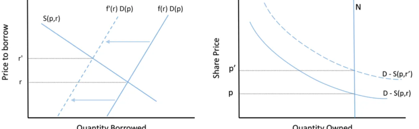
1.1 Tax Arbitrage Impact in the Stock Loan Market: Upper and lower panel depicts, respectively, the Average Daily Fee and Loan Interest for Petrobras (PETR4). Dotted lines, in red, indicate the record date of IoNE-dividend distribution events. . . 27 1.2 Typical Dates Flowchart for the IoNE Dividend Event: . . . 28 1.3 Difference Between Short-selling and Tax-Arbitrage Operations: 29 1.4 Simultaneous Determination of Stock Price and Loan Rate:

Simple framework based on Blocher et al. (2013). Left panel represents the equity loan market. The right figure displays the stock market. . . 29 1.5 Effects of the Tax Arbitrage: Left panel represents the speculative loan

market. Right panel shows the stock market. . . 30 1.6 Changes in Loan Fee Distribution Through Time: For each year,

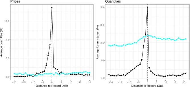
between January 2007 and June 2013, we plot the distribution of loan fees by firms. The vertical axis shows the frequency of firms with loan fees in the interval reported on the horizontal axis. . . 30 1.7 Fees and Loan-interest Around IoNE Dividend Events: The tax

arbitrage opportunity severely disrupts the stock loan market. Figure shows changes in prices and quantities. The horizontal axis depicts the distance to the record date. Left panel displays the average loan fee. For each stock, we calculate the daily loan fee as the value weighed fee among all contracts in a certain day. The figure shows the average daily loan fee among all stocks for each day around IoNE record dates. In a similar fashion, the chart on the right side displays the average loan-interest among shares. We consider 534 IoNE dividend events from January 2010 until June 2013. . . 31 1.8 Arbitrage vs Speculative Contracts: The top panel repeats the same

procedures as in Figure 1.7, but here we separate contracts into arbitrage (black) and speculative driven (red). Arbitrage loan contracts are the ones that have tax benefits - i.e, (1) borrowers are domestic investment funds and lenders are either retail investors or foreign investors, and (2) those contracts took place before the record date and were liquidated after it. We denote the remaining contracts speculative contracts. Lower panel is simply a zoomed version of the top panel. . . 32 1.9 Abnormal Returns Around The IoNE Dividend Date: For each

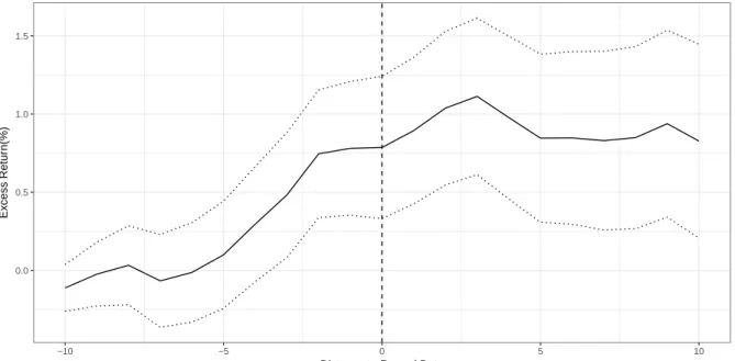
pair stock-event, we calculate the cumulative abnormal return starting 10 days before the record date. Figure shows the average cumulative abnormal return among 534 events. Abnormal return is calculated as the excess return over the IBRX50 index, which accounts for the 50 largest stocks in market capitalization. The dotted line represents the 95% confidence interval. 33 1.10 Reduced Form Coefficient for Different Return Windows: The

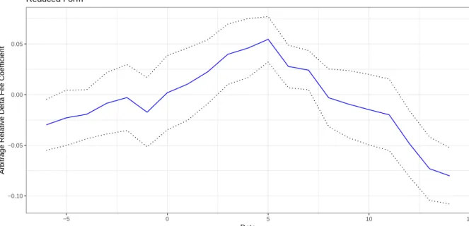
dependent variable of our regressions is the cumulative abnormal return. Figure shows how the estimated coefficient of Arb∆F ee responds to changes in the window where the cumulative return was calculated. X-axis indicates the final date of 9-days cumulative returns, y-axis is the coefficient of Arb∆F ee in reduced form regressions when considering as independent variables Arb∆F ee and controls. The dotted line is the 95% percent confidence interval. . . 34

(13)

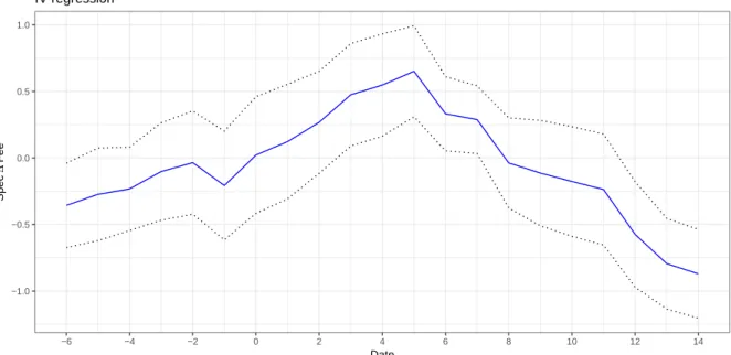
1.11 Second Stage Coefficient for Different Return Windows: The dependent variable of our regressions is the cumulative abnormal return. Figure shows how the estimated coefficient of Spec∆F ee responds to changes in the window where the cumulative return was calculated. X-axis indicates the final date of 9-days cumulative returns, y-X-axis is the coefficient of Spec∆F ee in structural form regressions when considering just one instrument: Arb∆F ee and controls. The dotted line is the 95% percent confidence interval. . . 35 1.12 Placebo Vs Treatment: Figure shows a comparison between IoNE and

Standard dividend events. Standard dividend events, in which there is no tax-arbitrage opportunity, are represented in light blue. IoNE dividents depicted in black. In both charts, the x-axis depicts the distance to the record date. Left panel shows the Average Loan Fee. For each stock, we calculate the daily loan fee as the value weighed fee among all contracts in a certain day. Average Loan Fee refers to the mean daily loan fee among stocks. In a similar fashion, the chart on the right side displays the average Loan-interest among shares. We consider 253 standard dividend events (blue) and 534 IoNE dividend events (black), from January 2010 until June 2013. . . 36 1.13 Abnormal Returns Around the Normal Dividend Date: Figure

shows the cumulative abnormal returns starting from 10 days previous record date. Abnormal return is calculated as the stock excess return over the IBX50 index, which accounts for the first 50 biggest stocks in market capitalization. The dotted line is the 95% percent confidence interval. . . 37 2.1 PETR4 Loan Contracts: Each dot represents a lending contract for

Petrobras (PETR4). The y-axis shows the loan fee paid for that contract. The x-axis depicts time. Note how for the same stock, on the same day, different investors are closing contracts with extremely different fees. . . . 67 2.2 Average Fee Range per stock: For each stock, we calculate the

average FeeRange across time. To be more specific, Fee Range assumes a (potentially) different value for each pair month-stock. In that sense, we could write F eeRange(t,stock). The chart bellow plots F eeRange(stock)

highlighting the cross sectional variation in Fee Range. . . 67 2.3 Time series of FeeRange, SI and AvgFee: For each month we

calculate the Aggregated Fee Range as the average Fee Range across stocks. Aggregate Short Interest and Aggregate Avg Fee were estimated in a similar fashion. As usual every month-stock measure, e.g. Fee Range, was calculated using the methodology described in Table 2.1. . . 68 2.4 Loan Contracts for PETR4: Color indicates the borrower type. We

group Commercial Banks, Pension Funds and other investors into the category "Other", which represents less than 8% of the total number of contracts. Each dot represents a lending contract for PETR4, and the y-axis shows the loan fee paid. . . 68 2.5 Total Monthly Financial Volume By Investor Type: . . . 69 2.6 Differences in Fees Between Investors: Evolution of loan fee spread

relatively to domestic funds, i.e. the difference betweeen the average fee paid by an investor group when compared to domestic funds. . . 70

(14)

2.7 Within Broker Fee Dispersion: We focus on the largest broker in terms of financial volume and include only the 274102 contracts that had him as intermediary. For each pair day-stock, Fee Range is calculated as the distance between the maximum and minimum fee. We also exclude any pair day-stock where less than 2 transactions took place. . . 71 2.9 Differences in Fees Between Brokers: We run a panel regression with

broker, ticker and date fixed effects. The dependent variable is the contract fee. Figure displays estimated fixed effects for the 30 largest brokers in terms of financial volume. We omit the estimated fixed effect for the remaining 90 (smallest) brokers. For each broker, the red line indicates the upper and the lower limit of the 95% confidence interval. Robust standard errors corrected for heteroskedasticity. . . 71 2.8 Daily Fee Range and Daily Average Fee: Figure displays, in black,

the time series of weighted average lending fee for selected stocks (GFSA3, JBSS3, RSID3). The blue ribbon indicates, for each day, the range of fees. In order to calculate those variables we consider only contracts initiated on that day, ignoring contracts that are active, but were negotiated in a different date. . . 72 2.10 Financial Volume Fixed Effects: We sort transactions into 100

quantiles accordingly to financial volume. The chart indicates the fixed effect for those quantiles, which were estimated through a panel regression with fixed effects for ticker, date and financial volume quantiles. The dependent variable is the contract fee. The 95% confidence interval, depicted in red, was estimated using robust standard errors corrected for heteroskedasticity. 73 2.11 Cumulative Returns for each long-short portfolio: . . . 74 2.12 Number of Stocks in Each Portfolio: . . . 75 2.13 Transition Matrix: The figure plots the transition probabilities of stocks

across the three range-fee sorted buckets over the period of one month. For example, the first column shows the percentage of stocks in the first bucket that end up in each of the three buckets after one month. . . 75 2.14 Correlation Matrix: The chart reports the time-series average correlation

between different variables. As an example, each month we estimate the correlation between Fee Range and Avg Fee. Denote this correlation as θt. That first step produced a time series of θt. Each cell in the upper

triangle matrix depicts the average θt for a given pair of measures. The

lower triangle part of the matrix reports the same information, but in graphic form. Each cell is shaded blue or red depending on the sign of the correlation, and with the intensity of color scaled 0–100% in proportion to the magnitude of the correlation. Circles‘ size are proportional to the absolute value of the correlation. Range refers to FeeRange, SD to SD-Fee, Avg to AvgSD-Fee, SI to short interest, Vol to Fee Volatility, Between to Range-Between and Within to Range-Within. . . 76 2.15 Loan Contracts for Gafisa (GFSA3): Color indicates the borrower

type: Foreign Investor, Domestic Fund, Retail Investors and Other. We group Commercial Banks, Pension Funds and other investors into the category "Other", which represents less than 8% of the total number of contracts. Each dot represents a lending contract for GFSA3. The y-axis shows the loan fee paid for that contract. The x-axis depicts time. . . 86

(15)

2.16 Time series of fee quantiles: The solid line (in black) represents the median fee. Maximum and minimum fees are depicted by dashed lines. Finally, red and blue ribbons highlight the changes in interquantile ranges throught the time series. JBS is ranked 111 in market cap out of 154 stocks in our sample, i.e. JBS is among the 30% largest companies . . . 87 3.1 Number of Active Investors: Figure displays the number of active

investors each month, for each investor group. We consider an investor to be active if she made at least one transaction on that month. Panel B changes the scale of the y axis allowing for a better visualization of the number active investors for the Foreign and BFF groups . . . 99 3.2 Number of Trades per month: Table displays the time series of the

total number of trades per month by each investor group. . . 101 3.3 Time series of FeeRange, SI and AvgFee: For each month we

calculate the Aggregated Fee Range as the average Fee Range across stocks. Aggregate Short Interest and Aggregate Avg Fee were estimated in a similar fashion. As usual every month-stock measure, e.g. Fee Range, was calculated using the methodology described in Table 2.1. . . 109 3.4 Number of Trades per Day: Table displays the time series of the total

(16)

List of Tables

1.1 Summary Statistics - Brazilian Equity Loan Market: Number of stocks refers to the number of different companies with shares traded in the stock loan market in a certain year. Volume is the financial volume, i.e. price times number of shares of all stocks lent, expressed in billions. For each stock, we calculate the daily loan fee as the value weighed fee among all contracts in a certain day. Then we calculate the yearly loan fee, for each stock, as the average daily loan fee. Table displays, for each year, the median yearly loan fee and average yearly loan fee among stocks. Loan Interest represents the number of shares, as a percentage of outstanding, on loan. The daily loan-interest for a specific stock is number of shares on loan at that day, normalized by the total number of shares outstanding. For each stock, we calculate the yearly loan interest as the average daily loan interest. Table displays, for each year, the average yearly loan interest among stocks. . . 38 1.2 Summary Statistics for Arbitrage Events: For each of the 534 IoNE

dividend events ir our sample, we calculate the following variables. Abnormal Return (AR) is the cumulative abnormal return using the stock’s closing prices from days -4 to +5, where the record day is defined as date 0. In other words, initial and final closing prices are 10 trading days apart. Daily stock abnormal return is the stock return minus the IBRX50, an index for the Brazian stocks traded at the stock exchange. Arbitrage∆F ee is the proportional increase in loan fees inside the event [−4, 0] with respect to a reference fee estimated outside the event[−21, −17]. The event fee is the average daily fee from -4 to 0. The reference fee is the average daily fee from -21 to -17. To calculate both, the event fee and the reference fee, we consider only contracts where the borrower is taxable (T), but the lender is non-taxable (NT). Spec∆F ee is calculated in analogous way but using only contracts with the remaining possible matchings of borrowers and lenders’ type (T-T, NT-T, NT-NT). Arbitrage Loan Interest is a proxy for the number of contracts allocated to tax-arbitrage transactions. It measures the amount of shares, as a proportion of outstanding, that satisfy the following conditions: (i) borrowers are tax-exempt while lenders are not and (ii) contracts were initiated before the record date and liquidated after it. We call those Arbitrage loan contracts because they generated riskless gains for borrowers. The remaining contracts are called Speculative. IoNE is the dividend yield, calculated as the payout value (per share) as a percentage of the ex-date price. Illiquidity is the daily-illiquidity average during the 252 business days before the event, where daily-illiquidity is calculated as in Amihud (2002). Log(MC) is the log of total market capitalization at the record date. Turnover is the average daily turnover (for that stock) in the 21 business days before the IoNE dividend record date. The daily turnover is the traded volume in a day, normalized by the market capitalization. For each stock, Median Fee is the median of average daily loan fee in the whole sample, whereas average daily loan fee is the value weighted average loan fee in a day. Similarly, Median LI is the median Loan Interest for the whole sample. . . 39

(17)

1.3 Reduced Form Results: Dependent variable is the stock’s cumulative abnormal return, calculated using the stock’s closing prices from days -4 to +5, where the record day is defined as date 0. Daily stock abnormal return is the stock return minus the IBRX50. Arbitrage∆F ee is the proportional increase in loan fees during the event with respect to a reference fee. The event fee is the average daily fee from -4 to 0. The reference fee is the average daily fee from -21 to -17. To calculate both, the event fee and the reference fee, we consider only contracts where the borrower is taxable (T), but the lender is non-taxable (NT). Spec∆F ee is calculated in analogous way but using only contracts with the remaining possible matchings of borrowers and lenders’ type (T-T, NT-T, NT-NT). Arbitrage Loan Interest is a proxy for the number of contracts allocated to tax-arbitrage transactions. It measures the amount of shares, as a proportion of outstanding, that satisfy the following conditions: (i) borrowers are tax-exempt while lenders are not and (ii) contracts were initiated before the record date and liquidated after it. We call those Arbitrage loan contracts because they generated riskless gains for borrowers. The remaining contracts are called Speculative. Robust standard errors corrected by clustering at the stock level in parentheses. The estimated beta for the intercept was omitted. Check Table 1.2 for a more detailed description of the remaining variables.. . . 40 1.4 First Stage: Arbitrage∆F ee is the proportional increase in loan fees during the

event with respect to a reference fee. The event fee is the average daily fee from -4 to 0. The reference fee is the average daily fee from -21 to -17. To calculate both, the event fee and the reference fee, we consider only contracts where the borrower is taxable (T), but the lender is non-taxable (NT). Spec∆F ee is calculated in analogous way but using only contracts with the remaining possible matchings of borrowers and lenders’ type (T-T, NT-T, NT-NT). Arbitrage Loan Interest is a proxy for the number of contracts allocated to tax-arbitrage transactions. It measures the amount of shares, as a proportion of outstanding, that satisfy the following conditions: (i) borrowers are tax-exempt while lenders are not and (ii) contracts were initiated before the record date and liquidated after it. We call those Arbitrage loan contracts because they generated riskless gains for borrowers. The remaining contracts are called Speculative. The estimated beta for the intercept was omitted. Robust standard errors clustered at the stock level. Check Table 1.2 for a more detailed description of the variables. . . 41 1.5 Second Stage Regressions: The first three columns represent Second Stage

Regressions for different set of instruments. OLS results are reported in columns (4). The instruments used are: Arbitrage Loan-Interest (LI) and Arbitrage Relative Delta Fee (ArbFee), and the two together. Dependent variable is the stock’s cumulative abnormal return, calculated using the stock’s closing prices from four days before the record date to five days after it. Daily stock abnormal return is the stock return minus the IBRX50. IoNE is the dividend yield. The estimated beta for the intercept was omitted in this table. Robust standard errors are clustered at the stock level. Check Table 1.2 for a more detailed description of the variables. . . 42

(18)

1.6 Different Windows and Overpricing Reversal: In each column, the dependent variable is the abnormal stock return in a different period/window. In Column (3), we repeat the results of Table 1.5, in which returns were accumulated around record date [−4, 5]. The remaining columns represent five trading days shifts of that window, but the initial and final closing prices used to calculate returns are always 10 trading days apart. Arbitrage∆F ee is used as instrument for Speculative∆F ee. Arbitrage∆F ee refers to the increase, in percentage, of the daily average loan fee inside the event[−4, 0] relatively to a reference fee estimated outside the event [−21, −17] considering only contracts where the borrower is tax-exempt but the lender is not. The method for calculating Spec∆F ee is analogous but using speculative contracts. IoNE is the dividend yield. The estimated beta for the intercept was omitted in this table. Robust standard errors clustered at the stock level. Check Table 1.2 for a more detailed description of the variables. . . 43 1.7 Determinants of the Instrument: Arbitrage∆F ee is the proportional

increase in loan fees during the event with respect to a reference fee. The event fee is the average daily fee in the 5 business days preceding (and including) the record day. The reference fee is the average fee between 21 and 17 business days before the record date. To calculate both, the event fee and the reference fee, we consider only contracts where the borrower is taxable (T), but the lender is non-taxable (NT). IoNE is the dividend yield evaluated at the ex-date. LI Before is the average loan interest outside the event [−21, −17]. HI lender is the Herfindahl Index, i.e. the sum of the squares of the market shares of the lenders’ brokers, evaluated using the stock’s lending contracts initiated up to one year before the event. The definition of HI borrower is analogous. Robust standard errors clustered at the ticker level. Check Table 1.2 for a more detailed description of the variables . . . 44 1.8 Placebo Test - Summary Statistics for Standard Dividend Events:

Although there is not tax arbitrage involving standard dividend payments, we define arbitrage and speculative contracts in the same way as we did for IoNE-dividends. Variables are calculated using the exact same procedure as described in Table 1.2, but for the sample of 249 standard dividend events. In previous tables, the Dividend Yield was called IoNE to emphasize that it we were not referring to standard dividend events. . . 45 1.9 Placebo Test Using Standard Dividends – Reduced Form Results:

Standard-dividends are not taxable in Brazil. Therefore, we use standard dividends to construct a placebo test. For consistency, we define arbitrage and speculative contracts in the same way as we did for the IoNE events, despite the fact that there is no arbitrage in this case. Variables are calculated using the exact same procedure as described in Table 1.2, but for the sample of 249 standard dividend events. Dividend Yield is the payout value as a percentage of the ex-date price. Turnover is the average daily stock’s turnover in the 21 days before the standard dividend event. Robust standard errors clustered at the stock level in parentheses. Check Table 1.2 for a more detailed description of the variables . . . 46

(19)

1.10 Incomplete Price Drop - Second Stage Regressions: As a robustness test we restrict the analysis to cumulative returns accruing from the ex-dividend date onward, i.e. from the closing price two days before the record date to five days after it. IoNE is the payout value (per share) as a percentage of the ex-date price. Log(MC) is the log of Market Cap. Turnover is the average daily turnover in the 21 business days before IoNE record date. Daily turnover is the stock’s traded volume in a day normalized by Market Cap. Robust standard errors clustered at the stock level. Check Table 1.2 for a more detailed description of the variables . . . 47 2.1 Description of the main variables: . . . 77 2.2 Summary Statistics: This table reports summary statistics for the

main variables in our study. Short interest is the total number of borrowed shares over total shares outstanding. Each month, SD Fee is calculated as the monthly average of daily standard deviation of fees. Average Fee is the average value weighted loan fee. Market Cap is represented in Millions. Book-to-market ratio is calculated in the end of December of each year. The cases with negative book value are deleted. Check Table 2.1 for a detailed description of how those variables were calculated. . . 78 2.3 Average Statistics per Year: This table reports, for each year, the

number of observations, number of stocks and the yearly average value of: market capitalization (in millions), book to market ratio, fee range, fees standard deviation, short interest, average fee and fee volatility. Check Table 2.1 for a detailed description of how those variables were calculated. 78 2.4 Investor Participation Rate: Table represents the participation rate of

each investor group as a percentage of the total number of contracts and as a percentage of total financial volume. We group investors into four categories: Domestic funds, foreign, retail investors and other. The group other includes comercial banks, pension funds and insurance companies

among others. . . 79 2.5 Returns to Long Short Strategies: Rows are ordered by Sharpe Ratio.

At the end of each month, from January 2007 to June 2013, we independently sort all valid stocks into three quantiles (buckets) based on their loan fee dispersion, average loan fee, short interest and fee volatility. Using stocks in each characteristic bucket, we form value (equal) weighted portfolios. We also form a zero-investment long-short portfolio that buys the low characteristics and sells the high characteristics. For all portfolios, the holding period is one month. Note that strategies based in measures of fee dispersion (Range Fee and SD Fee) perform better than the remaining long short portfolios based on usual measures of short selling restriction. Sharpe index based on annualized returns. Check Table 2.1 for a detailed description of how those variables were calculated. . . 79

(20)

2.6 Summary of Portfolio characteristics: At the end of each month, from January 2007 to June 2013, we independently sort all valid stocks in three quantiles (buckets) based on their loan fee dispersion (FeeRange). We then form value weighted portfolios using stocks in each characteristic bucket. Holding period is one month. For each portfolio and each month we calculate the market cap weighted average (across stocks) of market capitalization, book to market ratio, short interest, return, return volatility, stock turnover and average lending fee. This table displays the time series average for each of those variables. . . 80 2.7 Returns to portfolio strategies based on Fee Range: This table

provides portfolio alphas and loading, sorted on Fee Range. At the end of each month, all the stocks are sorted into three quantile: small (bottom 30%), Middle (40%), large (top 30%) deciles based on their fee range at the end of each month. Portfolio returns are computed over the next month minus the monthly risk free rate - 30 day DI Swap. For the analysis we consider 5 factors: Market, Small Minus Big Factor (SMB), High Minus Low (HML), Winners Minus Losers (WML), Illiquid Minus Liquid (IML). The factors considered were extracted from NEFIN. Data runs from January 2007 to June 2013. ***, **, and * stands for significance level of 1%, 5% and 10%, respectively. . . 81 2.8 FamaMacBeth Regressions: Each month we run a cross-sectional

regression of stock returns on previous month: loan fee dispersion, average loan fee, short interest, fee volatility and a set of control variables known to predict returns. Those regressions generate a time series of coefficients, θt. Table displays the time series average of those coefficients. Standard

errors are adjusted using the usual Fama and MacBeth (1973) procedure with Newey West correction. . . 82 2.9 FamaMacBeth Regressions: Each month we run a cross-sectional

regression of stock returns on previous month: loan fee dispersion, average loan fee, short interest, fee volatility and a set of control variables known to predict returns that include log of market capitalization, log of book to market, reversal (defined as past month return) and momentum (defined as the cumulative holding-period return from month t-12 to t-2). Those regressions generate a time series of coefficients, θt. Table displays the time

series average of those coefficients. Standard errors are adjusted using the usual Fama and MacBeth (1973) procedure with Newey West correction. 83 2.10 FamaMacBeth Regressions: Each month we run a cross-sectional

regression of stock returns on previous month: loan fee dispersion and a set of control variables known to predict returns. Table displays the time series average of estimated coefficients. Standard errors are estimated with the usual Fama and MacBeth (1973) procedure and Newey West correction. 84 2.11 FamaMacBeth Regressions: Each month we run a cross-sectional

regression of stock returns on previous month: loan fee dispersion and a set of control variables known to predict returns. Table displays the time series average of estimated coefficients. Standard errors are estimated with the usual Fama and MacBeth (1973) procedure and Newey West correction. 85

(21)

2.12 Returns to portfolio strategies based on Loan Fee Dispersion: This table provides portfolio alphas and loading, sorted on Loan Fee Dispersion. At the end of each month, all the stocks are sorted into three quantile: small (bottom 30%), Middle (40%), large (top 30%) deciles based on their loan fee dispersion at the end of each month. Portfolio returns are computed over the next month minus the monthly risk free rate - 30 day DI Swap. For the analysis we consider 5 factors: Market, Small Minus Big Factor (SMB), High Minus Low (HML), Winners Minus Losers (WML), Illiquid Minus Liquid (IML). The factors considered were extracted from NEFIN. Data runs from January 2007 to June 2013. ***, **, and * stands for significance level of 1%, 5% and 10%, respectively. . 88 2.13 Returns to portfolio strategies based on Average Loan Fee: This

table provides portfolio alphas and loading, sorted on Average Loan Fee. At the end of each month, all the stocks are sorted into three quantile: small (bottom 30%), Middle (40%), large (top 30%) deciles based on their average loan fee at the end of each month. Portfolio returns are computed over the next month minus the monthly risk free rate - 30 day DI Swap. For the analysis we consider 5 factors: Market, Small Minus Big Factor (SMB), High Minus Low (HML), Winners Minus Losers (WML), Illiquid Minus Liquid (IML). The factors considered were extracted from NEFIN. Data runs from January 2007 to June 2013. ***, **, and * stands for significance level of 1%, 5% and 10%, respectively. . . 89 2.14 Returns to portfolio strategies based on Short Interest: This table

provides portfolio alphas and loading, sorted on Short Interest. At the end of each month, all the stocks are sorted into three quantile: small (bottom 30%), Middle (40%), large (top 30%) deciles based on their short interest at the end of each month. Portfolio returns are computed over the next month minus the monthly risk free rate - 30 day DI Swap. For the analysis we consider 5 factors: Market, Small Minus Big Factor (SMB), High Minus Low (HML), Winners Minus Losers (WML), Illiquid Minus Liquid (IML). The factors considered were extracted from NEFIN. Data runs from January 2007 to June 2013. ***, **, and * stands for significance level of 1%, 5% and 10%, respectively. . . 90 2.15 Returns to portfolio strategies based on Loan Fee Volatility: This

table provides portfolio alphas and loading, sorted on Loan Fee Volatility. At the end of each month, all the stocks are sorted into three quantile: small (bottom 30%), Middle (40%), large (top 30%) deciles based on their loan fee volatility at the end of each month. Portfolio returns are computed over the next month minus the monthly risk free rate - 30 day DI Swap. For the analysis we consider 5 factors: Market, Small Minus Big Factor (SMB), High Minus Low (HML), Winners Minus Losers (WML), Illiquid Minus Liquid (IML). The factors considered were extracted from NEFIN. Data runs from January 2007 to June 2013. ***, **, and * stands for significance level of 1%, 5% and 10%, respectively. . . 91 3.1 How trades are represented at the data set: . . . 95

(22)

3.2 Summary Statistics for Trades by Different Investor Categories: Data runs from January 2012 to December 2017. Columns 2-3 report the total number of trades, first in million and then as a percentage of the total. Column 4 (Column 5) shows the average number of shares (monetary value) per trade. Columns 6 - 11 provides the attributes of the average firm traded: market capitalization; book to market ratio; and past returns measured over several non-overlapping time frames. To make comparison easier we transform these attributes into decile ranks, see the text for details. 96 3.3 How often do Investors Trade: Table shows summary statistics for the

number of days with transactions. . . 98 3.4 Summary Statistics for Portfolio Holdings on Dec 2016: For each

investor’s portfolio we calculate: the number of stocks, total portfolio value (in R$), the average stock’s book to market ratio and market cap. Table reports averages and quantiles calculated across investors within the same investor category. We round market cap values to the nearest thousand. . 102 3.5 Investor Type and Performance of Trades: Table reports average

coefficients and Newey West correct errors (in parentheses) for Fama Macbeth regressions computed from 12 specifications of daily cross-sectional regressions. The dependent variable in the first stage of the two-stage procedure is the day t daily return of stock j for data point n if stock j was purchased (first three rows) or sold (second set of rows) in the formation period corresponding to the columns. The same-day return in column [0, 0] is computed from trade price to the closing price on day t. After collecting coefficient estimates from each day in the sample period, the second stage computes coefficient estimates and the associated Newey West corrected standard errors from the time-series of coefficients. Panel A (Panel B) reports the estimates without (with) controls. Coefficients denoted with *, **, *** are significant at the 10%, 5% and 1% level, respectively. . . 104

(23)

1 Short Selling Restrictions and Returns: A

Natural Experiment

Fernando Barbosa ∗ _{Marco Bonomo} † _{João M. P. De Mello}‡ _{Lira Mota}§ ¶

ABSTRACT

We show that increases in stock loan fees have strong causal impact on stock prices. We identify these effects by exploiting exogenous variation in loan fees generated by a tax arbitrage opportunity that existed in Brazil from 1995-2014. The tax arbitrage involved differential tax treatment on dividend payments depending on investor’s type. Our data set allows to distinguish between equity lending transactions motivated by tax-arbitrage from those with the purpose of short-selling the stock. Variation in loan fees on tax-motivated transactions were a source of repeated exogenous variation of borrowing fees in short-selling transactions.

JEL classification: G12, G14.

Keywords: Short-Selling Restrictions, Overpricing, Miller Effect, Tax Arbitrage, Natural Experiment

∗_{FGV EPGE, email: fernando.luz@outlook.com}

†_{Insper, email: marcoacb@insper.edu.br, work phone: +55 11 4504 2342}

‡_{Insper; Central Bank of Brazil, email: JoaoMPM@insper.edu.br, work phone: +55 11 4504 2342} §_{Columbia Business School email: lrm2174@columbia.edu}

¶_{We thank BM&FBovespa for the data, and comments from Heitor Almeida, Martijn Boons, Igor}

Cunha, Kent Daniel, Bruno Giovannetti, Harrison Hong, Felipe Iachan, Charles Jones, Pedro Saffi, Dejanir Silva and participants at the following meetings and seminars: 2015 Luso-Brazilian Meeting, 2015 SED, 2015 Brazilian Finance Meeting, 2015 Brazilian Econometric Meeting, 2016 ESEM, 2017 LAMES, Cambridge, Columbia Finance and Economics Coloquium, Columbia Finance PhD Seminar, Catholic-Lisbon, Illinois, Insper, EESP-FGV, Brasilia Catholic University, UFPe.

(24)

1.1 Introduction

Since the seminal article of Miller (1977), the impact of short-selling constraints on financial markets have been subject of numerous theoretical1 and empirical studies.2 A well known predicted effect is that the interaction between heterogeneous valuations and short-sale constraints would lead to prices superior to the average valuation. Thus, in a market with differences of opinion and short-sale constraints, both an increase in disagreement or in short-sale restrictions would pressure prices upwards.3 While several empirical papers have convincingly illustrated the effect of the variation in heterogeneity on stock prices, documenting the effect of variation of stock loans supply poses a greater challenge.

Identification of the causal impact of short-selling restrictions on returns has been elusive for two reasons: data unavailability and the shortage of identifiable exogenous variation in short-sale restrictions. The lack of data stems from the over-the-counter structure of the stock loan market. Proper measures of short-sale restriction are difficult to obtain due to endogeneity of loan fees and short-interest 4_{, which reflect demand and supply decisions.}

More exogenous proxies for short-sale constraints, such as institutional ownership, tend to show little variation at high frequency.

In this paper we estimate the causal impact of short-selling restrictions on stock returns. We take advantage of a unique dataset and exploit a source of exogenous variation in short-sale restrictions provided by a tax-arbitrage opportunity that existed in Brazil from 1995-2014. The arbitrage opportunity stemmed from the fact that domestic investment funds were exempted from income taxes on dividends received on their borrowed stocks, whereas other types of investors would be taxed if they did not lend out those stocks. Because we observe all equity loan transactions, including the investor type, we can distinguish between equity lending transactions motivated by tax-arbitrage from those

1_{e.g. Harrison and Kreps (1978), Diamond and Verrecchia (1987), Duffie et al. (2002), Scheinkman}

and Xiong (2003), Hong and Stein (2003), Hong et al. (2006), Blocher et al. (2013)

2_{e.g. Chen et al. (2002), Asquith et al. (2005a), Cohen et al. (2007), Saffi and Sigurdsson (2011),}

Beber and Pagano (2013), Boehmer et al. (2013), De-Losso et al. (2013), Kaplan et al. (2013), Prado et al. (2014)

3_{e.g. Boehme et al. (2006), Nagel (2005)}

4_{Short interest is the number of shares that have been sold as part of a short sale and have not been}

(25)

with the purpose of short-selling the stock. Variation in tax-motivated stock borrowing is a source of exogenous variation in tightness on the lending market for short-selling purposes. Given the over-the-counter structure, the increased tightness implies not that fees are higher, but also that stocks are harder to find.5 _{- two different aspects of increased}

short-sale constraints. We estimate the causal impact of variation in short-sale constraints on stock prices, by estimating the effect on stock prices of fluctuations in lending fees induced by variation in tightness due to tax arbitrage operations.

In most countries, market-wide data on stock lending transactions is simply not available, since lending services are provided over-the counter by big custodians. The Brazilian security lending market provides a unique opportunity to circumvent the difficulties with data. Similarly to other countries, investors face an opaque lending market with an over the counter structure. However, all lending transactions are registered at a centralized platform - the BM&FBovespa. Consequently, we have access to a unique data-set containing all lending transactions, and their characteristics, such as type of borrower and lender (individual investors, investment funds, etc.), contract length, borrowing fees, number of securities lent, among others.

An even more challenging obstacle is the fact that decisions to supply or demand equity loans are not random, but influenced by investors’ (unobserved) expectations of future returns. One cannot infer causality by associating lending fees - as a measure of short selling constraints - with returns because fees are determined in equilibrium. A well-known finding of the literature is that an increase in short-demand should predict price declines (Boehmer et al. (2008)). In this case, lending fees increase in response to the increased stock loan demand from short-sellers, generating the well documented negative relation between lending fees and stock returns (e.g. Cohen et al. (2007) and Drechsler and Drechsler (2014b)). However, an exogenous loan supply reduction should also increase lending fees, and according to the Miller hypothesis, increases overpricing. Thus, stock loan supply shocks should generate a positive relation between loan fees and stock prices, which we propose to measure. The tax arbitrage involving dividend payments in Brazil provided a rare instance where strong and repeated exogenous variation in the supply of loanable stocks generated a clear positive relation between lending fees and stock prices.

5_{Several recent papers link search costs and loan fees (e.g. Chague et al. (2017),Kolasinski et al.}

(26)

Brazilian firms distribute two types of dividends: standard dividends and IoNE dividends (Interest on Net Equity). The difference is in the tax treatment, standard dividends are not taxable. However, shareholders pay a 15% tax rate on IoNE dividends, with the exception of domestic funds. More precisely, a IoNE dividend paid by a certain stock was taxed or not depending on the stockholder type at the record date. If the stock change hands through a stock loan transaction before the record date, the borrower would be consider the stockholder for tax purposes.

A tax arbitrage operation would entail a domestic fund borrowing stocks from a taxable investor before the IoNE dividend record date, in order to receive the full amount of dividend without any tax deduction. Tax-exempt borrowers would return IoNE dividend payments to lenders discounted by taxes. Thus, borrowers would profit from the taxes foregone by the government, discounted by the borrowing fee.6

Those arbitrage opportunities put pressure on the stock lending market around IoNE dividend events, resulting in sharp increases in lending fees. The profit per share obtained by tax arbitrageurs depend only on the dividend per share net of loan fees. Thus, we can argue that the increase in lending activity for tax arbitrage purposes is not related to the transacting parts assessment about the future price evolution of the stock. Around dividend events, the tax arbitrage is so lucrative that arbitrageurs crowd out short sellers who need to borrow shares in order to short. During those dividend events, the tax-arbitrage opportunity, by occupying some of the supply of loanable shares, exogenously reduces the supply of shares for short-selling purposes. This quasi-natural experiment of negative shocks in the supply of loans for shorting stocks allows us to characterize a causal effect of increase in short-sale constraints on the stock price.

The identification of investors’ types in our sample, allow us to divide the stock loan contracts into two segments. Contracts where the borrowers are domestic funds, and lenders are taxable will be called arbitrage contracts. All other matchings of borrowers and lenders’ type would not generate arbitrage. Thus, those loans must be motivated for borrowers’ intent to sell short the stock. We will denominate them speculative contracts.

In examining the effect of variation in short-selling constraints on the stock price, we

6_{As we document below, lending fees were substantially higher in those arbitrage operations than in}

other periods. Then, foregone taxes were in fact shared among borrowers, lenders and brokers. It is out of the scope of this paper to analyze the determinants of this division.

(27)

choose lending fees in the speculative segment as a proxy to the degree of short-restriction. The lending fee is not only a relevant cost for short-sellers, but is correlated with search frictions, whose direct measure is not available (see Kolasinski et al. 2013 and Chague et al. 2017). However, the speculative lending fee (and overall tightness in the speculative lending market) is endogenous, and very influenced by short-sellers’ beliefs about future stock returns. On the other hand, around record dates for IoNE dividends, a sizable variation in loan-interest and fees of arbitrage contracts is engendered by the increased borrowing of stocks for use in the arbitrage operations whose profits do not depend on the stock performance. Tax-arbitrageurs crowd-out short-sellers, reducing the supply of shares to borrow and, consequently, causing an increase in lending fees (and tightness) in the speculative market. This induced rise in speculative lending fees reflect increased scarcity in the stock loan markets rather than more pessimistic views about the stock prospect. We capture the effect of the scarcity in the stock loan market on stock returns by the use of an IV estimation strategy where we project speculative loan fees on arbitrage loan fees and arbitrage loan-interest.

Our main findings are as follows. First, tightness in the tax-arbitrage segment causes abnormal returns in stock prices. We establish that higher lending fees in the tax-arbitrage segment imply larger stock abnormal returns during the days surrounding IoNE dividend events. An increase of one standard deviation in loan fees in the arbitrage segment is associated with a 0.58% abnormal return increase in the two weeks around IoNE dividend record dates, i.e. 14.89% per year.

Second, tightness in the tax-arbitrage segment spills over to the speculative segment. Larger lending fees in the tax-arbitrage segment lead to higher lending fees in the speculative segment. This is the mechanism through which the exogenous shock propagates to stock prices, and constitutes the first stage of the IV estimation procedure we implement.7

Third, we use the increase in lending fees in the tax-arbitrage segment as an instrument to estimate the causal effect of (speculative segment) lending fees on stock prices. 8 _During

IoNE dividend distribution events, an average increase in speculative lending fees causes

7_{It is in principle possible that tightness in the speculative segment spills over to the arbitrage one.}

However, our empirical results indicate that around the record date it is mainly the arbitrage segment that influences the speculative one.

8_{We chose the arbitrage segment lending fee as the best instrument among our candidates with base}

(28)

a 0.55% (14% per year) abnormal return in the stock.9

Finally we show that the effect on the stock price happens only during the loan market tightness, reverting after the pressure on this market is released. More specifically, we experiment with different 9-day windows for the stock return, showing that the effect on stock returns happens only in the window that includes the record day. Moreover the loan tightness effect on the spot price is reverted between 7 and 15 days after the record date. Since we have many repeated similar events in our sample, this amounts to multiple instances of the Miller mechanism in place with stock price increases and decreases following the cycle of tightness and release in its loan market.

The timing of the effect also eliminates concerns that those changes in stock prices could be reflecting tax-motivated transactions in the spot market. Any spot market transaction motivated by the tax status of the dividend recipient should happen before or at the cum-day, which is three days before the record date. However, when we compute abnormal returns for days preceding the record date no effect is found. As a robustness test, we also repeat our main estimation with cumulative returns accruing from ex-dividend date onward and our results are maintained. Since, in one hand, no effects are found at the timing which could reflect dividend-related spot market operations and, at the other hand, our main results are confirmed for a timing that excludes any dividend-motivated spot market transaction, we can safely conclude that the results are only due to variations in loan market tightness induced by tax arbitrage.

By calculating returns from the ex-date forward, we also address concerns that our results could be contaminated by the ex-dividend abnormal return associated with phenomenon known as incomplete price drop, whereby stock’s prices drop by less than the dividend amount.10. In principle, the positive abnormal return associated with the incomplete price drop could induce a reduction in short-selling activity,as pointed out by Thornock (2013). Thus, in this case, causality would run from (expected) returns to short-selling activity, not the opposite.

As a an additional robustness test, we investigate whether the effects we found are related

9_{Since endogenous variation of loan fees would induce a negative correlation between loan fees and}

returns, we could consider our estimate as a lower bound for the effect of the exogenous variation of loan fees in returns.

(29)

to dividend payments, but unrelated to the tax arbitrage operations. In order to test this, we perform the same empirical exercise around the record date for nontaxable dividends. When dividends are nontaxable there is no tax arbitrage involving their payment. Therefore, one should not observe any extraordinary tightness in the stock loan market. If our effects were related to the dividend payment, but not to the tax arbitrage, we should obtain similar results in the estimation around record dates for nontaxable dividends. Thus, this constitutes a placebo test for our main effect. In contrast to our main results, the estimated reduced form coefficients for arbitrage fee and loan interest were negative. This is what we should expect since, in the absence of tax arbitrage, tightness in the loan market should reflect negative views about future stock returns. Again, this reinforces that the positive coefficients obtained reflect the causal effect of stressed loan markets on stock prices.

The paper is organized as follows. Section 1.2 contains a review of the literature. Section 1.3 gives an overview of the market for stock loans in Brazil. In Section 1.4 we describe the tax arbitrage opportunity in the period surrounding the IoNE payment dates and explain the transmission of its effect on short-selling and the stock price. In Section 1.3 we describe the data used for the paper. In Section 1.5 we present our empirical methodology. The results are analyzed in section 1.6. Section 1.7 presents robustness tests. The last Section concludes.

1.2 Related Literature

Our paper aims to measure the effect of changes in the supply of lendable shares on stock returns. In order to estimate the causal effect, the challenge is to identify shifts that are exogenous to changes in beliefs about stock returns.

On the theoretical side, several papers argue that - under different hypothesis - short selling restrictions can cause overpricing. Examples include Harrison and Kreps (1978),Scheinkman and Xiong (2003),Duffie et al. (2002) and Blocher et al. (2013). However, multiple empirical papers have failed to find a consistent relationship between short supply and stock returns. We highlight here the work by Kaplan et al. (2013) who conduct a true randomized experiment and find no evidence that supply shocks affect returns. Other

(30)

examples include Cohen et al. (2007) and Boehmer et al. (2013).

Cohen et al. (2007) tried to isolate the effects of stock loan supply and demand shifts on stock prices. They postulate that higher fees associated with increases in lending indicate a (net) increase in the demand for shorting. Increases in fees coupled with reductions in lending represent a supply shock. They found no significant effect of loan supply shocks on returns. Their identification strategy implicitly assumes that supply shocks do not contain any information about returns, which can be a strong assumption in some settings.

Chague et al. (2014) also try to separate shifts in short demand from shifts in lending supply. They take advantage of a unique data set that allows them to observe a significant part of the lending supply for a group of relatively small firms. In contrast with Cohen et al. (2007), they find that loan supply shocks have a significant effect on stock returns.

Boehmer et al. (2013) explores the short-sale ban of 2008 of more than 1,000 stocks, and contrary to Miller’s prediction, find no price bump for these stocks. Their identification strategy is to match banned stocks with similar stocks that have never suffered the ban. However, the choice of stocks in ban list was not randomly selected. Therefore, exogeneity with respect to beliefs about their future performance is not assured.

Kaplan et al. (2013) perform a field experiment, randomly increasing the supply of stocks available for lending by a particular money manager. They find almost no impact on outcome variables such as returns and bid-ask spreads. Experimental data provides convincing exogenous variation. But the supply shock may be too small to produce a quantitatively relevant impact.

Blocher et al. (2013) propose a reduced form framework for analyzing the equity loan market’s impact on share prices. In their model, shifts in loan supply have an impact on share prices only for hard-to-borrow stocks. Our results confirm their model’s prediction, since our tax-arbitrage induced negative supply shock is sizable enough to make loan supply binding for most stocks.

In more recent paper, Grullon et al. (2015) find support for the Miller Hypothesis. They examine a once for all relaxation of short-sale constraints (Regulation SHO), which released the uptick rule for a random sample of stocks. They found that prices for the treated stocks fall relatively to the control group, resulting in equity issues and investment reductions

(31)

for those stocks. However, because the fall happens two weeks before the announcement, the mechanism underlying the effect is unclear. Furthermore, they are not able to identify whether the effect is due to overpricing reversal or to coordinated short-selling attacks.

Our paper is also related to Thornock (2013), who show that a differential tax treatment between actual and substitute dividends leads to a contraction in the supply of lendable shares around the dividend record date. This makes the market tighter around the record date, with higher stock loan fees. Although Thornock (2013) and Blocher et al. (2013) document abnormal returns around the ex-dividend date, their empirical exercises do not relate them to any measure of the loan market tightness around the record date. Moreover, by measuring the abnormal return around the ex-date their results are subject to the confounding effect of the incomplete price-drop phenomenon.

We contribute to the literature by documenting repeated instances where increases in the cost of short-selling can cause overpricing. Our data enables us to disentangle two equity lending markets: one where stocks are borrowed for tax arbitrage operations (the tax arbitrage market) and other where stocks are borrowed for short-selling the stock. The tax-arbitrage opportunity, an exogenous shock, causes tightness in tax-arbitrage segment of the stock loan market, which leads to tightness in the speculative segment, which, in turn, causes abnormal returns. We measure the loan tightness shock in the speculative market through the projection of its loan fee on the arbitrage market loan fee. Our natural experiment also provides repeated instances of this shock, with the overpricing effect reversing after it.

1.3 Stock Loan Market in Brazil

Trading in equity loan market in Brazil is over-the-counter (OTC), as in most countries. Differently from other countries, all loan contracts must be registered with BM&FBovespa, the only stock exchange in Brazil. BM&FBovespa acts as a clearing platform, and as a central counterpart. It guarantees all loan contracts and keeps track of the contract collateral. Although investors face an opaque market, we had access to market-wide data, observing every single transaction.

(32)

lender, the borrower, the lender’s broker and the borrower’s broker. The cost to borrow a stock is the loan fee (which includes both brokers commission fees), plus an exchange fee of 0.25% annually.

Table 1.1 contains summary statistics about the Brazilian equity loan market from 2007 through 2013. In this period, the number of stocks lent fluctuated around 350. Just for comparison, the total number of listed stocks reached a peak in 2007 with 404 different companies. Therefore, most of the stocks were lent at least once. Other statistics indicate that the stock loan market gained importance in this period. The average annual growth in the volume of equity lending was 16%. The average loan-interest more than doubled, reaching 1.65% in 2013 11_{. The median loan fee dropped by an average 51 basis points}

(bps) per year, from 6.01% to 2.91%. On the lending side, retail investors, domestic investment funds and foreign investors represented approximately 90% of the market. Borrowers were mostly domestic investment funds (56.7%) and foreign investors (27.8%)

Figure 1.6 depicts the distribution of average loan fees for each stock for each year from 2007 to 2013.12 _{Fees were high as compared to more mature economies, with large proportion}

of fees exceeding 4% a year. However, one can observe that the whole distribution has been shifting to the left.

1.3.1 Data set

BM&FBovespa keeps detailed records of all lending transactions. The data set runs from January 2010 to June 2013 and we observe all of the 6,580,394 stock lending contracts closed in that period. We use the following data: contract date, liquidation date, loan fee, quantity of shares and investor type. This allow us to distinguish transactions that are eligible for tax arbitrage operations from those that are not13_.

In order to investigate changes in the lending market around taxable dividend distribution events, we focus on loan contracts in a window around those events, i.e. 21 days before and after each record date. Payout record dates were extracted from Quantum Axis.

11_{Loan-interest is number of shares held in loan contracts normalized by the total number of shares}

outstanding, this measure is calculated first daily, then yearly, for each stock and the average presented is the simple mean of the yearly loan-interest among stocks.

12_{The data for 2013 is an average of the first six months of the year.} 13_{See section 1.4 for a formal definition of tax-arbitrage contracts}

(33)

Information on stocks returns, traded volume and market cap are from Economatica.

The taxable type of dividend, which we call IoNE dividend (Interest on Net Equity), is treated as fixed income for tax purposes. The other type of dividend, or standard dividend, is exempt from taxes. IoNE dividend events have to satisfy certain criteria to be in the sample. There must be arbitrage contracts starting within the five days before the record date of the event, stocks must have been traded during all 21 trading days before and after the record date. We also require data on turnover during all 21 trading days before the record date and trim outliers by discarding the 0.5% highest and lowest returns in the sample14_{. The final sample has 534 events which include stocks representing}

approximately 70% of BM&FBovespa market capitalization. Table 1.2 contains summary statistics for those events.

Summary statistics hint at our main results. Stocks show an average 0.53% return over the IBRX50 index in a 9-trading-day period around IoNE dividend events, but dispersion is large. Loan-interest increases drastically during the event window. Fees on arbitrage contracts increase sixfold, reflecting the fact that lenders appropriate part of the tax arbitrage profit. Fees on speculative contracts also increase significantly, 99%. The average IoNE dividend yield is 0.96%.

1.4 The Tax Arbitrage and its Effect on the Stock Loan

Market

Figure 1.1 indicates that the stock loan market experiences an extreme level of distress around dividend payment events. The upper panel depicts the daily average lending fee for Petrobras stock, one of the largest companies in Brazil. Through most of the sample, lending fees oscillate close to 2%, but they soar around record dates, frequently reaching more than 15%. Lower panel shows that the amount of stocks lending also increases substantially around the record date. Petrobras is a liquid stock and one of the shares with highest financial turnover at the Brazilian stock exchange. In this type of environment, recurrent fee spikes, as those displayed in Figure 1.1, should not to be expected. The

14_{For robustness, we also trimmed at the following cutoffs: 0%, 2,5%. Results are similar and are}

(34)

cause of those was a tax arbitrage opportunity involving dividend payments. In the next subsections, we describe in detail the relevant dates for dividend distribution, the tax arbitrage operation, and how it generated intense stock lending activity around record dates.

1.4.1 Relevant dates for dividend distribution

Relevant dates for dividend distribution in Brazil are similar to those in the United States. Figure 1.2 depicts the flowchart of important dates for our empirical exercise in a typical IoNE distribution event.

The first date is the earnings’ announcement day, an official public statement of a company’s information for a specific time period, typically a quarter. On earnings’ announcement date investors get to know the company’s distribution policy, including the amount of payouts in the form of standard and IoNE dividends.

The second date is the payout announcement day (also called the declaration day), when the next IoNE dividend record and payment dates are announced. The payout announcement usually happens a month after the earnings’ announcement.

The record date day determines eligibility to the IoNE dividend. Holders of the stock as shown in the company’s books at the record date are entitled to the IoNE dividend. The ex-date day is the first day shares trade, at the spot market, without the right to receive the dividend. It is two days before the record date, since only three days after a spot market transaction the buyer’s name is added to the record book. The ex-date is at least one business day after the payout announcement. Finally, the payment date is when the IoNE dividend payment is made. The payment date varies considerably.

Notice that, differently from spot market transactions, lending transactions are registered immediately. Thus, if an investor borrows the stock between the ex-date and the record date, she will be entitled to receive the dividend payment, although a buyer in the spot market with the same timing would not have this same right.

(35)

1.4.2 The Tax Arbitrage Opportunity

Until August 2014, a difference in tax treatment between distinct investors generated a tax arbitrage opportunity.15 _{Since the borrower was considered the owner of the stock for}

tax purposes, non-taxable funds could borrow a stock from a taxable investor during the period of its IoNE dividend distribution and receive the full dividend amount. They had to pay the original stockholder only the dividend net of the 15% of taxes, retaining the difference. 16 17

Figure 1.3 illustrates the difference between a short-sell and a tax-arbitrage operation. At the upper panel, investor A is holding a long position and acts as lender. Investor B borrows shares from A and short-sell them to C. Investor C has the right to receive the actual dividends paid by the stock. However, the lender (A) will receive the same value, in the form of cash dividends, paid by the borrower (B). At the lower panel, investor B borrows the stock, but there is no short-sell. The arbitrageur(B) is a non-taxable investor and, therefore, will receive the full dividend amount div. However, if the lender (A) is a taxable investor, she has the right to receive only 0.85*div as cash dividends. The loophole in the tax law transferred money from the government to non-taxable investors.18

In Brazil, the law requires a minimum distribution of 25% of profits. Brazilian firms distribute profits through two types of dividend: standard and IoNE (Interest on Net Equity). Firms prefer to distribute profits through IoNE dividends because they are deductible from profits for tax purposes, representing a tax shield. 19 Hence, payment of IoNE dividends to stockholders is widely used by firms in Brazil. Our final sample includes 534 IoNE dividend distribution events.

15_{Under a new law, non-taxable investors should pay taxes on IoNE dividends if their shares were}

obtained by borrowing them from a taxable investor

16_{Tax exemption was given to domestic funds and investment clubs in order to avoid double taxation}

on the funds’ shareholders, which had their NAVs appreciation already taxed.

17_{In order to avoid confusion, it is worth pointing out that Chague et al. (2017) depicts a slightly}

incorrect description of IoNE tax rates. They write "individual investors pay a tax rate of 15% while financial institutions are exempt". Actually, foreign financial instutions are not exempt.

18_{In practice, non-taxable investors share with taxable investors and brokers the amount of taxes}

subtracted from the government through the borrowing and fees they pay.

19_{However, there is an upper limit to the amount of IoNE dividends a firm can distribute, but not to the}

amount of standard dividends. Firms can distribute IoNE dividends up to the smaller of three following numbers: the net worth times the Long-Term Interest Rate (a prime rate determined by the federal government), 50% of the current period earnings before corporate taxes, and 50% of the accumulated earnings and reserves in previous periods. Details on the differences between both types of dividends can be found at the appendix.