Camila Valéria de Jesus SILVA1

(1)

Floristic and structure of an Amazonian primary forest

and a chronosequence of secondary succession

Camila Valéria de Jesus SILVA*1_{, João Roberto dos SANTOS}1_{, Lênio Soares GALVÃO}1_, Ricardo Dal’Agnol da SILVA1_{, Yhasmin Mendes MOURA}1

1 _{Instituto Nacional de Pesquisas Espaciais, Divisão de Sensoriamento Remoto, Avenida dos Astronautas, 1758, Jardim da Granja,}

São José dos Campos, SP, Brasil. CEP:12227-010.

* _{Corresponding author: camilaflorestal@gmail.com}

ABSTRACT

The analysis of changes in species composition and vegetation structure in chronosequences improves knowledge on the regeneration patterns following land abandonment in the Amazon. Here, the objective was to perform floristic-structural analysis in mature forests (with/without timber exploitation) and secondary successions (initial, intermediate and advanced vegetation regrowth) in the Tapajós region. The regrowth age and plot locations were determined using Landsat-5/Thematic Mapper images (1984-2012). For floristic analysis, we determined the sample sufficiency and the Shannon-Weaver (H’), Pielou evenness (J), Value of Importance (VI) and Fisher’s alpha (α) indices. We applied the Non-metric Multidimensional Scaling (NMDS) for similarity ordination. For structural analysis, the diameter at the breast height (DBH), total tree height (Ht), basal area (BA) and the aboveground biomass (AGB) were obtained. We inspected the differences in floristic-structural attributes using Tukey and Kolmogorov-Smirnov tests. The results showed an increase in the H’, J and α indices from initial regrowth to mature forests of the order of 47%, 33% and 91%, respectively. The advanced regrowth had more species in common with the intermediate stage than with the mature forest. Statistically significant differences between initial and intermediate stages (p<0.05) were observed for DBH, BA and Ht. The recovery of carbon stocks showed an AGB variation from 14.97 t ha-1

(initial regrowth) to 321.47 t ha-1_{(mature forests). In addition to AGB, Ht was also important to discriminate the typologies.} KEYWORDS:Forest recovery; vegetation dynamics; forest structure; floristic patterns, biomass.

Florística e estrutura de uma floresta primária e uma cronossequência de

sucessão secundária na Amazônia

RESUMO

A análise de mudanças na composição de espécies e estrutura da vegetação em cronosseqüências aprimora o conhecimento sobre os padrões de regeneração após o abandono das terras na Amazônia. Nosso objetivo foi realizar análise florístico-estrutural em florestas maduras (com / sem exploração madeireira) e em sucessões secundárias (inicial, intermediária e avançada) na região do Tapajós. A idade da regeneração e os locais das parcelas foram determinados usando imagens Landsat-5 TM (1984-2012). Na análise florística, foi determinada a suficiência amostral e os índices de Shannon-Weaver (H’), uniformidade de Pielou (J), Valor de Importância (VI) e alfa de Fisher (α). Foi aplicada análise de escalonamento multidimensional não-métrico (NMDS) para ordenação de similaridade. Na análise estrutural, o diâmetro à altura do peito (DAP), altura total da árvore (Ht), área basal (BA) e biomassa acima do solo (AGB) foram obtidos. As diferenças entre tipologias dos atributos florísticos-estruturais foram verificadas utilizando os testes de Tukey e Kolmogorov-Smirnov. Os resultados mostraram aumento dos índices H’, J e alfa a partir da sucessão inicial até as florestas maduras da ordem de 47%, 33% e 91%, respectivamente. O estágio avançado apresentou mais espécies em comum com o estágio intermediário do que com a floresta madura. Foram observadas diferenças estatisticamente significativas entre os estágios iniciais e intermediários (p <0,05) para o DAP, BA e Ht. O retorno dos estoques de carbono mostrou uma variação de AGB de 14,97 t ha-1_{(estágio inicial) para 321,47 t ha}-1_{(florestas maduras). Além de}

AGB, Ht também foi um atributo importante para discriminar as tipologias.

(2)

INTRODUCTION

Severe modifications of the biophysical characteristics of primary forests result from their conversion into agriculture areas and livestock. There are also further effects from timber logging and forest fires (Asner et al. 2005; Aragão et al. 2008; Xaud et al. 2013). On the other hand, livestock grazing areas intensively exploited in the past and subsequently abandoned are in process of natural regeneration.

Several orbital remote sensing studies using optical (Lucas

et al. 2002; Lu 2005) or radar data (Santos et al. 2009; Saatchi

et al. 2011) have contributed for the characterization and

monitoring of primary (with and without timber exploitation) and secondary forests at the local and regional scales. However, floristic and structural analysis is still essential to investigate and better understand the regeneration process of vegetation following land abandonment in the Amazon region.

Analytical procedures based on floristic diversity and on measurements of structural parameters have been traditionally performed. Projects whose objective is the discriminatory study of forests with some type of disturbance such as selective logging or fires have contributed for such measurements (Martins et al. 2012). In the specific case of the differentiation between successional stages, these studies include variables related to age of regeneration and land use history (Mesquita

et al. 2001; Araújo et al. 2005; Salomão et al. 2012). The age

of regeneration is an attribute that facilitates the classification of secondary succession stages (Lu et al. 2003). However, this attribute is not easily determined due to the influence of other factors on vegetation regrowth such as the soil structure, precipitation patterns, clearing size and land use history. Moreover, the distance from the primary forest matrix and the presence of fauna dispersing seeds have been reported as important factors to affect the growth rate and biomass accumulation during the regeneration process (Chazdon et al. 2007).

In order to minimize the effects of these environmental factors, studies of chronosequences have been performed in tropical forests. A chronosequence is composed of sites formed from the same parent material that differ over time. In other words, the sites present similarities with respect to soil types and environmental conditions, climate zone and are affected by land-use history or disturbance (Chazdon 2012). Thus, under controlled environmental conditions, it is possible to describe differences in successional trajectories through the detailed quantification of floristic composition and forest structure (Mesquita et al. 2001).

The Tapajós National Forest (FLONA Tapajós), located in Brazil, has been extensively studied using satellite images (Santos et al. 2003; Espírito-Santo et al. 2005; Galvão et al. 2009). However, only a few studies in the FLONA Tapajós

and surroundings have focused on the classification of secondary succession stages. Further studies are necessary to know how and to what extent the floristic-structural attributes differ among the stages and with respect to mature forests. This is especially important in the context of a new legislation system in the state of Pará (Instrução

Normativa 02/2014 - DOE/PA Nº 32594) that regulates

the management of secondary forests at different stages of vegetation regeneration to reduce the deforestation of primary forests. Secondary forests occupy more than 165,000 km2_and

are highly dynamic components of complex mosaics in this Brazilian state (Vieira et al. 2014). This work contributes to improve the knowledge on how to distinguish the secondary stages, supporting the government policies and inspection. In this context, the objective of this study was to analyze floristic-structural differences between mature forests (with and without timber exploitation) and a chronosequence representative of three stages of secondary succession (initial, intermediate and advanced) in the Tapajós region.

MATERIALS AND METHODS

The study area comprises the northern part of the Tapajós National Forest (Brazilian state of Pará) and its surroundings, situated between the latitudes 2º_{53’06” S and 3}º_{11’ 48” S, and}

the longitudes 54º_{47’35” W and 55}º_{01’03” W. According to}

the Köppen classification, the climate is Ami – wet tropical, with the annual average temperature and precipitation of 25°C and 1820 mm, respectively.

The region is characterized by low rolling relief, comprising the lower Amazon plateau and the upper Xingu-Tapajós plateau. The Tapajós Forest is dominated by primary tropical rainforest with emergent trees and a uniform vegetation cover (Dense Ombrophilous Forest). Some areas have dissected plateaus with a few emerging trees and a high density of palm trees (Open Ombrophilous Forest). The predominant soil types are Dystrophic Yellow Latosol and Red-Yellow Podzolic soils. Historically, the land use in the surroundings consists of subsistence agriculture, a few cash crops, cattle husbandry and selective logging activities, but there is currently a large land conversion to extensive areas of agriculture (maize, rice, soybeans) outside the FLONA.

Forest inventory plots were surveyed in August 2012 to analyze floristic-structural differences between Initial (SSI), Intermediate (SSInt) and Advanced (SSA) Secondary Successions; Forest with Timber Exploitation (FPEM); and Primary Forest (FP). The vegetation age is the most straightforward approach for the discrimination of regeneration stages (Saldarriaga et al. 1988). In the present study, we adopted the age interval proposed by Lu et al.

(3)

intermediate (SSInt between 6 and 15 yr), and (3) advanced (SSA with > 15 yr). Areas of primary forest (FP) and also forest with disturbance arising from legal logging (FPEM) formed a baseline to assess the magnitude of the changes in floristic and structural attributes over time and of the regenerative capability of the successional process. In the FPEM area, selective logging of trees with DBH greater than 45 cm was performed in 1979, when 75 m³ ha-1_{of wood was exploited}

(Costa Filho etal. 1980).

The locationof the representative samples of all typologies under investigation was determined through the analysis of Landsat-5/Thematic Mapper (TM) satellite images acquired between 1984 and 2012. The images also allowed verification of: (1) the occurrence of forest fragmentation in the study area; (2) the existence of disturbances in the primary forest; (3) the potentials impact of logging effects; and, in some cases, (4) the forest conversion period and age of the secondary succession. In the absence of evidence from these satellite images to monitor the time of successional chronosequence, ground information was obtained from the local community on the land use and year of the last clearance.

In the field survey, 40 transects were defined with a total area of 6.4 ha. For the FP, FPEM and SSA, the dimension of each plot was 25 m x 100 m. For the SSI and SSInt, the plot size was 20 m x 50 m. All transects were positioned geographically using a Global Positioning System (GPS). The information on the past land use and land cover (LULC) history and the predominant classes (LULC matrix) around the surveyed secondary succession plots were obtained from the TerraClass Project (www.inpe.br/cra/projetos_pesquisas/terraclass2008. php). The information is summarized in Table 1.

The forest inventory considered all the trees with Diameter at the Breast Height (DBH) > 10 cm, except for the SSInt and SSI typologies (DBH ≥ 5 cm). Following the procedures adopted by Gonçalves and Santos (2008), we also estimated the total and commercial tree heights.

All the species were identified with the assistance of a parabotanist with a vast experience in the regional flora. The scientific and family names were confirmed using the “Brazilian Species Name Index 2013” (http://floradobrasil.jbrj.gov.br/) and the database of the Missouri Botanical Garden 2013 (http:// www.tropicos.org). Individuals of the Arecaceae were excluded from the sampling.

The sample sufficiency was assessed by rarefaction curve based on sampling units generated by 1000 randomizations computed using the EstimateS software (version 9, R. K. Colwell, http://purl.oclc.org/estimates). The construction of the rarefaction curve is an interpolation process from the species richness of the full set of samples, for the expected richness of a subset of that sample (Colwell et al. 2004). This curve increases until the point where the increase in sampling units does not add new species. At this point, the sampling is considered sufficient for inclusion of almost all species present in the area.

The floristic composition was analyzed between the typologies using the Shannon-Weaver (H’) and Pielou evenness (J) indices, proposed by Odum (1983) and Magurran (1988), which express the floristic diversity of the sampled area. In addition, to compare the typologies without the effect of the sampling size, we calculated also the average values of the Fisher’s alpha index (Magurran 1988). We evaluated their differences using the ANOVA and post-hoc Tukey test with a significance level of 5%. We estimated the phytosociological parameters of density, dominance and frequency, which provided the measure of the value of importance (VI) by species. The NMDS (Non-metric Multidimensional Scaling), a multivariate method for ordination analysis (Gauch 1982), was applied to evaluate the floristic similarity between the typologies. The NMDS was based on the species abundance and Bray-Curtis distance. This method reduces a multidimensional dataset into a one-dimension space, showing the plots with high species similarity and placing far apart those plots with low similarity. A subsequent analysis was performed to test if all the plots of each typology were grouped together in an ellipse of 95%

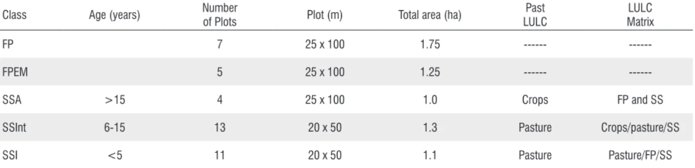
Table 1. Sampling effort for primary and secondary forests: (1) primary forest (FP); (2) forest with timber exploitation (FPEM); (3) advanced secondary succession (SSA); (4) intermediate secondary succession (SSInt); and (5) initial secondary succession (SSI). The past land use and land cover (LULC) and the predominant classes (matrix) around the studied SS plots are indicated.

Class Age (years) Number

of Plots Plot (m) Total area (ha)

Past LULC

LULC Matrix

FP 7 25 x 100 1.75 ---

---FPEM 5 25 x 100 1.25 ---

---SSA >15 4 25 x 100 1.0 Crops FP and SS

SSInt 6-15 13 20 x 50 1.3 Pasture Crops/pasture/SS

(4)

confidence interval based on the standard deviation of scores. The NMDS was performed using the R 3.2.0 vegan and MASS packages, and the standard deviation ellipses were made using the cluster package.

For the structural characterization, we established diametric classes with a range of 5 cm and calculated the basal area (BA). The allometric equations for estimating the aboveground biomass (AGB) differed between the forest typologies and secondary successions (Table 2). A specific allometric equation

for Cecropia sp. was used for the plots dominated by this specie.

To inspect for differences in vegetation structure between the typologies, we performed statistical tests over DBH, Ht, BA and AGB. We used a non-parametric statistical analysis (Kolmogorov-Smirnov test). These procedures allow verifying if there is a similarity in the variable distribution by each vegetation typology and, when not, which variables differ from each other.

RESULTS

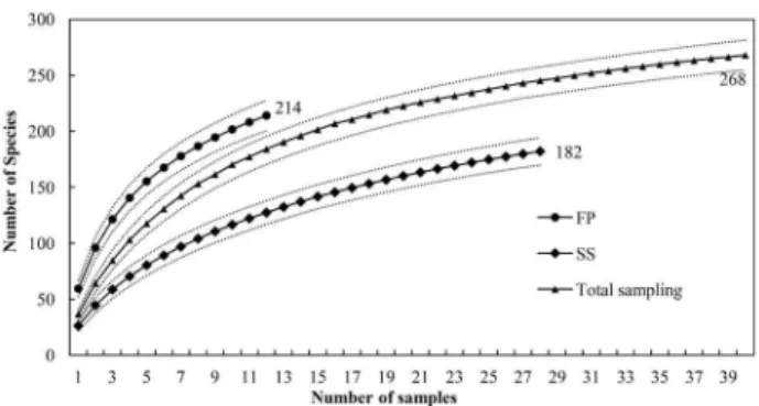
During the floristic survey, we identified 4,277 individuals and 268 species (supplementary material) distributed in 56 families in 6.4 ha of area. The stability of the rarefaction curve based on the number of accumulated sampling units was especially observed for the secondary forests. Obviously, this occurs because the primary forest exhibits greater richness of species. The analysis of rarefaction curves showed that the proportions of new species were below 5% of the species recorded in the last samples, considering the mean curve estimated for each different forest typology (Figure 1).

The successional chronosequence presented increased values of H’ from 2.44 to 4.36 for the young and old regrowth stages (Table 3). Similar tendency was observed for the J values (0.60 to 0.90). This indicated that the most advanced stage of the chronosequence was approaching the value of diversity (H’ = 4.61) found in the primary forest, while having already reached the same level in terms of evenness (J = 0.90).

The average Fisher’s alpha index values increased from SS1 (4.23) to FP (49.57) (Table 3). The statistical post-hoc Tukey test (p < 0.05) revealed that the typologies FP and FPEM

formed a group with equivalent values of average diversity. Statistically, the SSA, SSInt and SSI typologies presented a very distinct average diversity, making possible the distinction between them, as well as from the aforementioned group. This result showed that SSA did not reach the species diversity found in FP. We identified as outliers one plot of SSInt having 50 species and another from SSI with just 5 species. In terms of diversity, the SSInt resembled the SSA. The SSI was dominated

by Cecropia palmata (95% of the individuals), making it very

distinct from the other samples.

Ten species with higher VI (%) were ranked according to the typology (supplementary material). FP, FPEM and SSA had common species as observed also for SSInt and SSI. The

Figure 1. Curves of species accumulation based on the number of samples (solid lines), and their respective confidence intervals (α = 0.05) for the representative samples of forests (with or without timber exploitation) and secondary successions. The solid black line (middle) expresses the representation of the entire set of inventoried samples without considering the stratification by vegetation typology

Table 2. Allometric equations used for estimating the aboveground biomass (AGB).

Class Equation Source

FP, FPEM y = 0.0509 x ρ D² HT Chave et

al. 2005* SSA, SSInt,

SSI Y = exp(-2.17+(1.02x(LnDAP²))+(0.39xLn(Ht)) Uhl et al. 1988

Cecropia

ssp. Y= exp(-2.5118 + 2.4257 x Ln DAP)

Nelson et al. 1999 * ρ = 0.69 (Fearnside, 1997)

Table 3. Floristic attributes of each forest typology. Abbreviations: N = Abundance; NF = number of botanical families; S = number of species; α = Fisher’s alpha index average (standard deviation) and Tukey test (p<0.05); H’ = Shannon-Weaver index; and Pielou evenness index = J.

Class N NF S α H´ J

FP 857 40 181 49.57(8.1) a 4.61 0.89

FPEM 553 40 139 47.32(6.5) a 4.43 0.90

SSA 472 38 125 34.30(10.2) b 4.36 0.90

SSInt 1345 42 128 14.30(7.0) c 3.90 0.80

(5)

species Couratari stellata (tauari) was well distributed in all the sampled plots of FP and SSA. We did not find this species in the plots disturbed by old selective logging activities. Thus, it is an important species for forest recovery of the deforested areas, present in the list of species of the chronosequence, including the most advanced stage. It is a potential species for timber management. In the FP and FPEM plots, the species Protium hebetatum (breu-vermelho) was abundant. However, in the FPEM plots, this species presented trees with small basal area, probably resulting from management due to its economic potential.

Despite the low basal area, the pioneer species Cecropia

palmata (embaúba-branca), Casearia grandiflora (sardinheira),

Swartzia flaemingii (tento-flamengo) and Vismia guianensis

(lacre-branco) had large numbers of individuals. All of them were present in the forest chronosequence, especially in the initial and intermediate stages of secondary succession. Even in the SSA plots, the species Cecropia palmata had significant abundance (59 trees) when compared to other species. In spite of being a pioneer species colonizing environments with good light availability, it remains in the forest structure even in the advanced stage of regeneration with great competition between species.

The species Inga alba (ingá-vermelho), Guatteria

schomburgkiana (envira-preta) and Jacaranda copaia

(pará-pará) were observed in many SSInt and SSA plots.

Tapirira guianensis (tapiririca) was identified only in the

SSA, occupying the ninth place in the rank of the largest VI percentages.

In the NMDS analysis, 77% of the variance was captured in the first dimension. By adding the second dimension, 84% of the data variance was explained. The groups, represented by the ellipses, showed the similarity of the plots considering only the species composition (Figure 2). There was a separation of the FP and FPEM groups, but with the presence of some plots with high floristic similarity. For the secondary succession, there was a distinction between the groups, but an overlapping area was observed showing the transition process during the succession. The SSA plots presented higher floristic similarity with the SSInt plots than with FP/FPEM plots. Two of eleven SSI plots were grouped together with the SSInt plots.

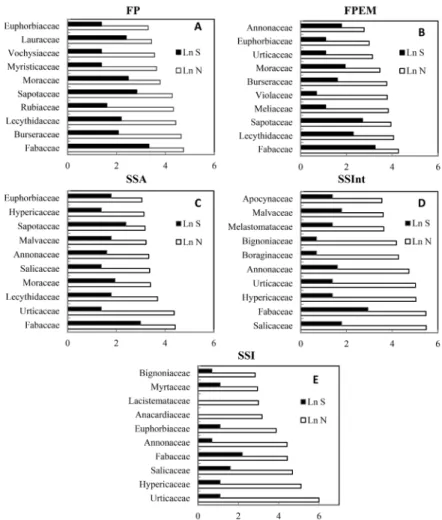
There were common botanical families between the five typological classes. However, they diverged in terms of quantity of individuals and species (Figure 3), as well as in height of stands. This was a characteristic of the entire successional chronosequence until the mature forest. The Fabaceae was significantly present in all successional stages. It comprised the largest number of individuals and species, ranging from 13 to 18% in the four largest forest structure classes. In the initial stages of the chronosequence (SSI),

the Fabaceae also included a greater number of species. The Urticaceae (38.5%) and Hypericaceae (16.5%) families showed greater abundance, whereas the Lacistemataceae presented the lowest richness in SSI.

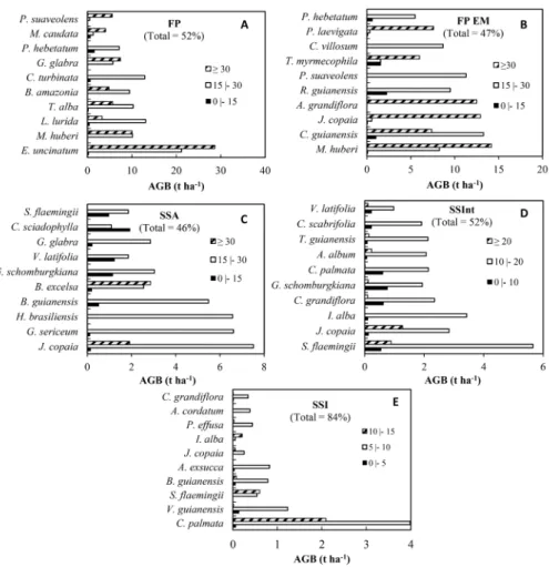
To illustrate the contribution of each species in the calculation of the AGB by typology, the ten largest biomass estimates were related to the height of individuals (Figure 4). The first analysis showed the transition of one stratum to the next with changes in successional stage. The species C. palmata

and V. guianensis and A. excusa occurred in SSI and were replaced in SSInt by other species with greater biomass accumulation in the upper height strata such as S. flaemingii, J. copaia and I. alba.

In the SSA, the species J. copaia, G. sericeum (quinarana),

B. guianensis (tatajuba)and H. brasiliensis (seringueira) greatly contributed to the biomass content (between 5 and 7.5 t ha-1₎

in the vertical intermediate stratum from 15 to 30 m. The increment of the biomass values resulting from the increase in height and basal area of the individuals of the J. copaia

species showed their ability to survive and dominate the canopy (vertical structure) as well as to disseminate individuals, expressed in the horizontal structure.

The selective logging areas (FPEM) accumulated greater biomass (total of 48%) in the vertical upper stratum (height above 30 m), with predominance of the species M. huberi

(maçaranduba), J. copaia and A. grandiflora (melancieira). In comparison with the FP (without timber exploitation), the FPEM exhibited greater biomass content (55%) in the intermediate stratum (between 15 and 30 m). The species E.

uncinatum (quarubarana) was the exception representing 15%

of the total biomass of the sampled area in FP, while being more representative in the upper canopy stratum in mature forest.

(6)

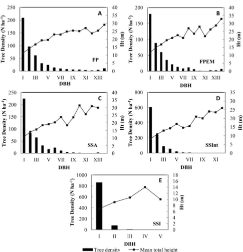
We further analyzed the structure of each typology through the diametric distribution of individuals and average height (Figure 5). The classes showed an inverted J distribution pattern in the diametric analysis and the number of trees of their respective intervals, the configuration of which occurs in all strata from the intermediate chronosequence (SSInt). As expected, the exception was the early stages of succession, in which there was a concentration of individuals in lower diametric intervals.

With respect to the recovery of carbon stocks during the successional process, the average biomass for FP, FPEM, SSA, SSInt and SSI was 321.47 ± 40.07 t ha-1_{, 270.56 ± 28.11 t ha}-1_,

109.85 ± 21.21 t ha-1_{, 75.06 ± 22.34 t ha}-1_{and, 14.97 ± 4.27}

t ha-1_{, respectively. From the AGB estimates, we inferred that}

the average annual increase of this biophysical attribute was 3.0 t ha-1

.yr-1 in the initial stages of succession and 5.7 t ha-1 yr-1

in the intermediary stage. The value declined to 4.0 t ha-1 _yr-1

when the process reached the advanced stage.

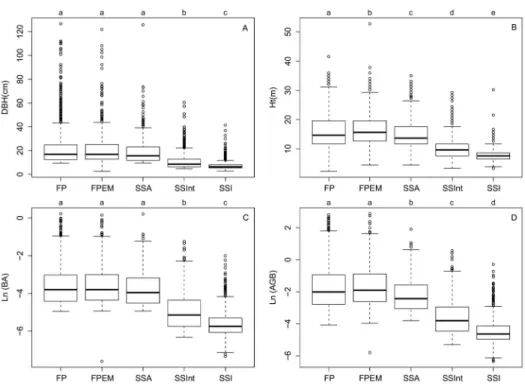
When the distribution of population was considered in the analysis, the two-sample Kolmogorov-Smirnov test (α = 0.05) showed pronounced differences between SSInt and SSI for the DBH, Ht and BA attributes (Figure 6). The analysis of the DBH and BA showed statistical differences between SSInt and SSI, and similarity between FP, FPEM and SSA. AGB presented differences between SSA, SSInt and SSI and similarities between FP and FPEM. Ht was an important attribute to differentiate all typologies, which needs to be better considered in further studies of successional stages.

DISCUSSION

The sampling is sufficient when an increase of 10% in area corresponds to an increase of less than 10% in new species (Schilling and Batista 2008).The slightly stability of the rarefaction curve is observed with a trend to an asymptote, as reported by Carim et al. (2007). Thus, in our study, all forest typologies were sufficiently sampled. However, some authors indicate basal area as a much more important attribute than the

(7)

number of new species to define the sampling size, especially if the objective is the assessment of forest structure (Mueller-Dombois and Ellenberg 1974; Magurran 1988).

In general, our values of H’ and J were close to those found in other studies in the region (Espírito-Santo et al. 2005; Rodrigues et al. 2007; Gonçalves and Santos 2008). These indices are sensitive to sample size, but they have been used by several researchers (Magurran 1988). Our results with the Fisher’s alpha index, which does not depend on the sampling size, were generally concordant with the H’ and J indices, but highlighted the differences between the typologies.

The NMDS analysis showed that 84% of the species abundance information of all the typologies was captured in two dimensions. The first dimension has a pronounced gradient where the majority of the species abundance information was summarized (77%). On this gradient, the species distribution and its abundance defined the successional group formation, which is represented by the distance or dissimilarity between the plots. In general, the lower values of the first NMDS dimension

represented the primary forest plots, while the higher values were related to the secondary forest plots. Although the NMDS scores have no biophysical meaning, they showed a clear distinction of the successional groups represented by a measure of how similar the groups were based on the species composition of each one. A further analysis could explore environmental variables to explain the distribution of the plots along this first NMDS dimension searching for the physical and chemical parameters that define the presence of certain species, but this analysis is out of the scope of this work.

This analysis revealed the group formation of the typologies, based on species composition, and added information to the diversity analysis. This is important because the successional stages were not separated only by their structural attributes, but also by their floristic aspects. The floristic aspects should be considered in conjunction with the structural attributes, in the governance of the secondary forest management. In this study, we found two SSI plots floristically similar to SSInt plots, and one of it would be susceptible to clearance following the new legislation.

(8)

Figure 5. Tree density (N ha-1_{) and mean total height (Ht), as a function of the intervals of diameter at breast height (DBH) for each forest typology; (A) – FP,}

(B) – FPEM, (C) – SSA, (D) – SSInt, (E) – SSI. For FP, FPEM and SSA the diameter classes were determined in intervals of 5 cm starting from DBH of 10 cm. For SSInt the first diameter class starts from 5 cm. For SSI the first diameter class starts from 2.5 cm, but the following classes were divided in 5 cm intervals. The Romans numbers in the horizontal axis represent the diameter classes.

Although the SSA diversity is significantly higher than the SSInt, these typologies were floristically similar, according to the NMDS analysis. As a result, it is relevant to highlight the ecological function of the intermediate secondary successions, because the species composition of these areas can compose a more complex environment. Therefore, our studied SSA plots have not recovered yet the floristic aspects observed in mature forests.

One of the assumptions of diversity measures is that all species are equal (Peet 1974). The taxonomic distinction is an alternative to show the distribution of the species in families. Baar et al. (2004) described the importance of the Fabaceae in the Amazonian forest, especially in the regeneration process, in which it had the highest species richness, abundance and basal area when compared to other botanic families. In our study, Fabaceae was the family with the largest abundance and distribution of species, having an important role on the succession process. In general, our results showed a large numbers of individuals and a reduced number of species between the families present in the SSInt and SSI classes.

The occurrence of specific dominant genera in the initial regenerative stage was important in the analysis.For instance, the presence of Cecropia and Vismia can explain the successional age, the ability of species recruitment, the differences in structure of the stands and the biomass allocation (Mesquita et al. 2001). According to these authors,

the Vismia species had slower growth in the height/diameter

ratio, thicker crowns and higher light interception than the

Cecropia species. While Vismia formed the closed-canopy

uniform layer, Cecropia species grew quickly and created a stratified canopy that allowed survival and growth of other tree species beneath its canopy, influencing second-growth forest structure.

(9)

2.6 t ha-1 _yr-1_{, 4.4 t ha}-1 _yr-1_{and 4.0 t ha}-1 _yr-1 _{were obtained,}

respectively. In addition to AGB, our results showed that the Ht was also an important biophysical attribute to differentiate the mature forest and successional stages. According to Moran and Brondı́zio (1998), who analyzed forest regeneration in four sites in the Brazilian state of Pará, the height of the stand was an important discriminator between the initial (5 yr), intermediate (10 yr) and advanced (over 15 yr) stages of secondary succession.

Height is a structural biophysical parameter estimated with high accuracy by remote sensing instruments like active microwave sensors (Treuhaft and Siqueira 2000) and LIDAR (Lefsky et al. 2005). The use of remote sensing for the acquisition of the height parameter over secondary forests is potentially important in the context of the new legislation system that regulates the clearance and conservation practices on secondary forests in the Pará state.

The ability of each species to occupy different dimensions in mature forests and secondary successions is important to explain the differences found in the abundance, richness and diversity of the individuals. This is also expressed in the functional characteristics of the horizontal and vertical structure of the forest typology, through variations in basal area and biomass content. It is important to mention that forest structure and its dynamics are strongly conditioned by spatial location, a key factor for the regulatory mechanisms of the Amazon floristic composition. Although a sufficient

number of forest inventories have been carried out in the Amazon to allow direct comparison of their results, the areas surveyed were generally susceptible to the influences of local hydrological, chemical and physical properties of the soil and land-use history. Thus, great caution is required when considering the broader implications of such comparisons among the areas. However, the results reported in this article are derived from surveys and analyses of the primary and secondary forest floristic and structure in the Tapajós region. They are comparable to those obtained by other authors and expand the knowledge of the Amazon forest with new local information.

CONCLUSIONS

In this study, we described the different stages of secondary succession through the analysis of their floristic-structural parameters. We showed that is possible to differentiate between the secondary successions stages, including advanced secondary regrowth from primary forests and forest with selective logging. Further studies are necessary to find out how long it takes for the secondary forests to recover the original species composition and diversity. Structurally, the three secondary succession stages can be clearly differentiated. As the total height was the only parameter by which was possible to differentiate all the typologies, the use of remote sensing instruments to estimate height, in the Amazonian forest landscapes, can support the government policies for

(10)

the management of natural secondary regrowth areas aiming at the reduction of the deforestation over the primary forest.

ACKNOWLEDGEMENTS

The authors are very grateful to the Coordenação de

Aperfeiçoamento de Pessoal de Nível Superior (CAPES),

Conselho Nacional de Desenvolvimento Científico e Tecnológico

(CNPq - Brazil) and Instituto Chico Mendes de Conservação

da Biodiversidade (ICMBio/MMA - Sisbio Process 35010-1).

Thanks are also due to Luiz Carlos Batista Lobato (CBO/Museu

Paraense Emílio Goeldi – MPEG) for fieldwork assistance in

botanical identification, and to Carlos Cordeiro and Gabriel Moulatlet (INPE) for assistance in statistical analysis. The logistic support provided by the Santarém Office of the Large Scale Biosphere-Atmosphere Experiment in Amazonia (LBA) was highly appreciated. Finally, the authors thank the anonymous reviewers for the nice suggestions.

REFERENCES

Aragão, L.E.O.C.; Malhi, Y.; Barbier, N.; Lima, A.; Shimabukuro, Y.; Anderson, L.; Saatchi, S. 2008. Interactions between rainfall, deforestation and fires during recent years in the Brazilian Amazonia. Philosophical Transactions of the Royal Society of London. Series B, Biological Sciences, 363: 1779–1785. Araújo, M.M.; Tucker, J.M.; Vasconcelos, S.S.; Zarin, D.J.; Oliveira,

W.; Sampaio, P.D.; Rangel-Vasconcelos, L.D.; Oliveira, F.A.; Coelho, R.F.R.; Aragão, D.V.; et al.. 2005. Padrão e processo sucessionais em florestas secundárias de diferentes idades na Amazônia Oriental. Ciência Florestal, 15: 343–357.

Asner, G.P.; Knapp, D.E.; Broadbent, E.N.; Oliveira, P.J.C.; Keller, M.; Silva, J.N. 2005. Selective logging in the Brazilian Amazon.

Science, 310: 480–482.

Baar, R.; Cordeiro, M. dos R.; Denich, M.; Folster, H. 2004. Floristic inventory of secondary vegetation in agricultural systems of East-Amazonia. Biodiversity and Conservation, 13: 501–528. Carim, S.; Schwartz, G.; Silva, M.F.F. 2007. Riqueza de espécies,

estrutura e composição florística de uma floresta secundária de 40 anos no leste da Amazônia. Acta Botanica Brasilica, 21: 293–308. Chave, J.; Andalo, C.; Brown, S.; Cairns, M.A.; Chambers, J.Q.;

Eamus, D.; et al. 2005. Tree allometry and improved estimation of carbon stocks and balance in tropical forests. Oecologia, 145: 87–99.

Chazdon, R. 2012. Regeneração de florestas tropicais Tropical forest regeneration. Boletim Museu Paraense Emílio Goeldi de Ciencias Naturais, 7: 195–218.

Chazdon, R.L.; Letcher, S.G.; Van Breugel, M.; Martínez-Ramos, M.; Bongers, F.; Finegan, B. 2007. Rates of change in tree communities of secondary Neotropical forests following major disturbances. Philosophical Transactions of the Royal Society of London. Series B, Biological Sciences, 362: 273–89.

Colwell, R.K.; Mao, C.X.; Chang, J. 2004. Interpolando, extrapolando y comparando las curvas de acumalación de especies basada en su incidencia. Ecology, 85: 2717–2727.

Costa Filho, P.; H. Costa; O. Aguiar, 1980. Exploraçao mecanizada da floresta tropical úmida sem babaçu, Embrapa-CPATU, Circular Técnica 9, Belém - PA.

Espírito-Santo, F.D.B.; Shimabukuro, Y.E.; Kuplich, T.M. 2005. Mapping forest successional stages following deforestation in Brazilian Amazonia using multi‐temporal Landsat images.

International Journal of Remote Sensing, 26: 635–642. Fearnside, P.M. 1997. Wood density for estimating forest biomass in

Brazilian Amazonia. Forest Ecology and Management, 90: 59–87. Galvão, L.S.; Ponzoni, F.J.; Liesenberg, V.; Santos, J.R.. 2009.

Possibilities of discriminating tropical secondary succession in Amazônia using hyperspectral and multiangular CHRIS/ PROBA data. International Journal of Applied Earth Observation and Geoinformation, 11: 8–14.

Gauch, H.G., Jr. 1982. Multivariate Analysis in Community Structure. Cambridge University Press, Cambridge, 1982, 312p. Gonçalves, F.G.; Santos, J.R. 2008. Composição florística e estrutura

de uma unidade de manejo florestal sustentável na Floresta Nacional do Tapajós, Pará. Acta Amazonica, 38: 229–244. Lefsky, M.A.; Harding, D.J.; Keller, M.; Cohen, W.B.; Carabajal,

C.C.; Espirito-Santo, F.D.B.; Hunter, M.O.; Oliveira Jr., R. 2005. Estimates of forest canopy height and aboveground biomass using ICESat. Geophysical Research Letters, 32: 1–4. Lu, D. 2005. Integration of vegetation inventory data and Landsat

TM image for vegetation classification in the western Brazilian Amazon. Forest Ecology and Management, 213: 369–383. Lu, D.; Mausel, P.; Brondı́zio, E.; Moran, E. 2003. Classification of

successional forest stages in the Brazilian Amazon basin. Forest Ecology and Management, 181: 301–312 .

Lucas, R.M.; Honzák, M.; Amaral, I.; Curran, P.J.; Foody, G.M. 2002. Forest regeneration on abandoned clearances in central Amazonia. International Journal of Remote Sensing, 23: 965–988. Magurran, A. 1988. Ecological diversity and its measurement.

Princeton, NJ, USA: Princeton University Press, 179p. Martins, F.S.R.V.; Xaud, H.A.M.; Santos, J.R.; Galvão, L. S. 2012.

Effects of fire on above-ground forest biomass in the northern Brazilian Amazon. Journal of Tropical Ecology, 28: 591–601. Mesquita, R.C.G.; Ickes, K.; Ganade, G.; Williamson, G.B. 2001.

Alternative successional pathways in the Amazon Basin. Journal of Ecology, 89: 528–537.

Moran, E.F.; Brondı́zio, E. 1998. Land-Use Change After Deforestation in Amazonia. In D. Liverman, E. F. Moran, R. R. Rindfuss, P. C. Stern (Eds.), People and Pixels: Linking Remote Sensing and Social Science. Washington DC: National Academy Press, p. 94–120.

Mueller-Dombois, D.; Ellenberg, G.H. 1974. Aims and methods of vegetation ecology. Chichester, England: John Wiley and Sons, Inc, 547p.

Nelson, B.W.; Mesquita, R.; Pereira, J.L.G.; Souza, S.G.A.; Batista, G.T.; Couto, L.B. 1999. Allometric regressions for improved estimate of secondary forest biomass in the central Amazon.

(11)

Odum, E.P. 1983. Ecologia. Editora Guanabara, Rio de Janeiro, 1983, 434p.

Peet, R.K. 1974. The measurement of species diversity. Annual Review of Ecology and Systematic, 5: 285-307.

Rodrigues, M.A.C.M.; Miranda, I.S.; Kato, M.S.A. 2007. Estrutura de florestas secundárias após dois diferentes sistemas agrícolas no nordeste do estado. Acta Amazonica, 37: 591–598.

Saatchi, S.; Marlier, M.; Chazdon, R.L.; Clark, D.B.; Russell, A.E. 2011. Impact of spatial variability of tropical forest structure on radar estimation of aboveground biomass. Remote Sensing of Environment, 115: 2836–2849.

Saldarriaga, J.G.; Darrel, C.W.; Tharp, M.L.; Uhl, C. 1988. Long-Term Chronosequence of Forest Succession in the Upper Rio Negro of Colombia and Venezuela. Journal of Ecology, 76: 938–958.

Salomão, R.P. 1994. Estimativas de biomassa e avaliação do estoque de carbono da vegetação de florestas primárias e secundárias de diversas idades (capoeiras) na Amazônia Oriental, município de Peixe-boi, Pará. Dissertação de Mestrado, Universidade Federal do Pará/ Museu Paraense Emilio Goeldi, Belém. 53p.

Salomão, R.D.P.; Vieira, I.C.G.; Júnior, S.B.; Amaral, D.D.; Santana, A.C. 2012. Sistema Capoeira Classe : uma proposta de sistema de classificação de estágios sucessionais de florestas secundárias para o estado do Pará. Boletim Museu Paraense Emílio Goeldi de Ciencias Naturais, 7: 297–317.

Santos, J.R.; Freitas, C.C.F.; Araujo, L.S.; Dutra, L.V; Mura, J.C.; Gama, F.F.; Soler, L.S.; Sant’Anna, S.J.S. 2003. Airborne P-band SAR applied to the aboveground biomass studies in the Brazilian tropical rainforest. Remote Sensing of Environment, 87: 482–493.

Santos, J.R.; Narvaes, I.S.; Graça, P.M.L.A.; Gonçalves, F.G. 2009. Polarimetric responses and scattering mechanisms of tropical forests in the Brazilian Amazon. In G. Jedlovec (Ed.), Advances on geoscience and remote sensing, Vukovar, Croatia: NASA/MSFC-USA, p. 183–206.

Schilling, A.C.; Batista, J.L.F. 2008. Curva de acumulação de espécies e suficiência amostral em florestas tropicais. Revista Brasileira de Botânica, 31: 179–187.

Treuhaft, R.N.; Siqueira, P.R. 2000. Vertical structure of vegetated land surfaces from interferometric and polarimetric radar. Radio Science, 35: 141–177.

Uhl, C.; Buschbacher, R.; Serrao, E.A.S. 1988. Abandoned Pastures in Eastern Amazonia. I . Patterns of Plant Succession. Journal of Ecology, 76: 663–681.

Vieira, I.C.G.; Gardner, T.A.; Ferreira, J.; Lees, A.C.; Barlow, J. 2014. Challenges of governing second-growth forests: A case study from the Amazonian state of Pará. Forests, 5: 1737-1752. Xaud, H.A.M.; Martins, F.S.R.; Santos, J.R. 2013. Tropical forest

degradation by mega-fires in the northern Brazilian Amazon.

Forest Ecology and Management, 294: 97–106.

(12)

Class Species N U AB DR FR DoA DoR VI (%)

FP

Erisma uncinatum 26 6 6.91 3.03 1.40 3.95 12.82 5.75

Protium hebetatum 56 7 2.03 6.53 1.63 1.16 3.76 3.98

Lecythis lurida 26 6 2.91 3.03 1.40 1.66 5.41 3.28

Tachigali alba 22 7 2.52 2.57 1.63 1.44 4.69 2.96

Coussarea grandifolia 55 4 0.78 6.42 0.93 0.45 1.45 2.93

Manilkara huberi 11 6 2.79 1.28 1.40 1.59 5.17 2.62

Couratari stellata 26 7 1.02 3.03 1.63 0.58 1.89 2.18

Chimarrhis turbinata 8 5 2.13 0.93 1.16 1.22 3.96 2.02

Goupia glabra 5 5 2.00 0.58 1.16 1.14 3.72 1.82

Iryanthera paraensis 21 6 0.76 2.45 1.40 0.43 1.41 1.75

Mabea caudata 19 3 0.90 2.22 0.70 0.51 1.66 1.53

Buchenavia amazonia 3 2 1.93 0.35 0.47 1.10 3.57 1.46

Protium paniculatum 17 7 0.42 1.98 1.63 0.24 0.77 1.46

Ecclinusa ramiflora 13 5 0.53 1.52 1.16 0.30 0.98 1.22

Mouriri collocarpa 8 5 0.78 0.93 1.16 0.44 1.44 1.18

Tetragastris panamensis 13 4 0.53 1.52 0.93 0.31 0.99 1.15

Virola michelii 11 5 0.53 1.28 1.16 0.30 0.98 1.14

Abarema mataybifolia 10 5 0.54 1.17 1.16 0.31 1.00 1.11

Eschweilera grandifolia 10 5 0.39 1.17 1.16 0.22 0.72 1.02

Helicostylis pedunculata 11 5 0.27 1.28 1.16 0.15 0.50 0.98

Inga thibaudiana 12 5 0.19 1.40 1.16 0.11 0.36 0.97

Ocotea glomerata 8 5 0.39 0.93 1.16 0.22 0.72 0.94

Duguetia stelechantha 8 5 0.32 0.93 1.16 0.18 0.59 0.90

Brosimum guianensis 8 5 0.28 0.93 1.16 0.16 0.52 0.87

Tachigali paniculata 8 4 0.38 0.93 0.93 0.22 0.71 0.86

Pouteria jariensis 8 5 0.23 0.93 1.16 0.13 0.43 0.84

Cordia scabrifolia 8 4 0.31 0.93 0.93 0.18 0.58 0.81

Tachigali myrmecophila 6 2 0.66 0.70 0.47 0.38 1.22 0.79

Pouteria macrophilla 9 4 0.19 1.05 0.93 0.11 0.36 0.78

Protium spruceanum 7 5 0.15 0.82 1.16 0.09 0.28 0.75

Trichilia micrantha 10 3 0.19 1.17 0.70 0.11 0.36 0.74

Pseudopiptadenia suaveolens 3 2 0.75 0.35 0.47 0.43 1.40 0.74

Eschweilera coriacea 7 1 0.62 0.82 0.23 0.36 1.16 0.74

Astronium gracile 4 3 0.55 0.47 0.70 0.31 1.02 0.73

Neea oppositifolia 7 4 0.20 0.82 0.93 0.12 0.37 0.71

Guarea guidonia 8 3 0.26 0.93 0.70 0.15 0.48 0.70

Minquartia guianensis 6 4 0.25 0.70 0.93 0.15 0.47 0.70

Eriotheca globosa 5 4 0.31 0.58 0.93 0.18 0.58 0.70

Qualea paraensis 4 2 0.61 0.47 0.47 0.35 1.14 0.69

Vochysia guianensis 3 3 0.54 0.35 0.70 0.31 1.01 0.68

Matayba guianensis 8 4 0.10 0.93 0.93 0.06 0.19 0.68

Guatteria schomburgkiana 7 4 0.15 0.82 0.93 0.08 0.27 0.67

Aparisthmium cordatum 6 5 0.08 0.70 1.16 0.05 0.15 0.67

Castilla ulei 6 4 0.15 0.70 0.93 0.09 0.28 0.64

Myrciaria floribunda 8 3 0.14 0.93 0.70 0.08 0.27 0.63

Bertholletia excelsa 1 1 0.83 0.12 0.23 0.47 1.54 0.63

SUPPLEMENTARY MATERIAL

Species with the highest Value of Importance (VI) ranked by forest typology and associated phytosociological parameters. Abbreviations: N = number of individuals; U = number of plots on which there was occurrence; AB = basal area; DR = relative density; FR = relative frequency; DoA = absolute dominance; DoR = relative dominance.

FP

Micropholis venulosa 2 2 0.63 0.23 0.47 0.36 1.18 0.62

Brosimum parinarioides 5 5 0.06 0.58 1.16 0.03 0.11 0.62

Endopleura uchi 5 4 0.17 0.58 0.93 0.10 0.32 0.61

Anacardium spruceanum 2 2 0.58 0.23 0.47 0.33 1.08 0.59

Maquira sclerophylla 3 3 0.39 0.35 0.70 0.23 0.73 0.59

Sterculia pruriens 5 3 0.26 0.58 0.70 0.15 0.48 0.59

Duguetia echinophora 7 3 0.13 0.82 0.70 0.07 0.24 0.59

Protium robustum 6 4 0.06 0.70 0.93 0.04 0.12 0.58

Apeiba echinata 5 2 0.37 0.58 0.47 0.21 0.68 0.58

Inga graciliflora 4 4 0.18 0.47 0.93 0.10 0.33 0.57

Calyptranthes bipennis 5 4 0.11 0.58 0.93 0.06 0.21 0.57

Aniba parviflora 6 3 0.18 0.70 0.70 0.10 0.32 0.57

Abarema piresii 4 3 0.26 0.47 0.70 0.15 0.48 0.55

Pouteria gongrijpii 3 3 0.31 0.35 0.70 0.18 0.58 0.54

Virola calophylla 5 3 0.15 0.58 0.70 0.08 0.27 0.52

Licaria aritu 4 3 0.20 0.47 0.70 0.12 0.38 0.51

Inga marginata 5 3 0.13 0.58 0.70 0.07 0.23 0.50

Eschweilera amazonica 7 2 0.12 0.82 0.47 0.07 0.22 0.50

Amaioua guianensis 7 2 0.10 0.82 0.47 0.06 0.19 0.49

Pouteria anibifolia 4 3 0.15 0.47 0.70 0.08 0.27 0.48

Licania heteromorpha 5 3 0.07 0.58 0.70 0.04 0.13 0.47

Micropholis acutangula 3 3 0.20 0.35 0.70 0.11 0.36 0.47

Pouteria cladantha 4 3 0.10 0.47 0.70 0.06 0.19 0.45

Lecythis pisonis 1 1 0.53 0.12 0.23 0.30 0.98 0.44

Swartzia arborescens 4 3 0.08 0.47 0.70 0.05 0.15 0.44

Laetia procera 2 2 0.32 0.23 0.47 0.18 0.60 0.43

Inga rubiginosa 4 3 0.06 0.47 0.70 0.04 0.11 0.43

Ambelania acida 4 3 0.05 0.47 0.70 0.03 0.10 0.42

Miconia pyrifolia 4 3 0.04 0.47 0.70 0.02 0.08 0.41

Poecilanthe effusa 4 3 0.04 0.47 0.70 0.02 0.08 0.41

Thyrsodium paraense 3 3 0.09 0.35 0.70 0.05 0.16 0.40

Roucheria punctata 5 2 0.07 0.58 0.47 0.04 0.13 0.39

Eugenia cupulata 5 2 0.07 0.58 0.47 0.04 0.13 0.39

Licania egleri 3 3 0.06 0.35 0.70 0.04 0.11 0.39

Sacoglottis guianensis 3 3 0.05 0.35 0.70 0.03 0.09 0.38

Pouteria guianensis 3 2 0.16 0.35 0.47 0.09 0.30 0.37

Ocotea canaliculata 3 2 0.16 0.35 0.47 0.09 0.29 0.37

Stryphnodendron guianensis 3 2 0.15 0.35 0.47 0.09 0.28 0.36

Protium apiculatum 2 2 0.19 0.23 0.47 0.11 0.35 0.35

Alibertia edulis 4 2 0.06 0.47 0.47 0.04 0.12 0.35

Rinorea racemosa 4 2 0.04 0.47 0.47 0.03 0.08 0.34

Siparuna decipiens 2 2 0.17 0.23 0.47 0.10 0.31 0.34

Eugenia brachypoda 3 2 0.10 0.35 0.47 0.06 0.19 0.33

Maytenus myrsinoides 1 1 0.34 0.12 0.23 0.20 0.64 0.33

Zygia racemosa 3 2 0.09 0.35 0.47 0.05 0.17 0.33

(13)

FP

Micropholis cuneata 2 2 0.15 0.23 0.47 0.09 0.28 0.33

Paypayrola grandiflora 3 2 0.09 0.35 0.47 0.05 0.16 0.33

Ocotea rubra 3 2 0.08 0.35 0.47 0.05 0.15 0.32

Parkia multijuga 1 1 0.33 0.12 0.23 0.19 0.60 0.32

Inga alba 3 2 0.06 0.35 0.47 0.04 0.12 0.31

Pouteria reticulata 2 2 0.12 0.23 0.47 0.07 0.23 0.31

Ormosia paraensis 2 2 0.11 0.23 0.47 0.07 0.21 0.30

Lacunaria jenmanii 3 2 0.05 0.35 0.47 0.03 0.09 0.30

Vatairea erythrocarpa 3 1 0.18 0.35 0.23 0.10 0.33 0.30

Symphonia globulifera 2 2 0.11 0.23 0.47 0.06 0.20 0.30

Aspidosperma spruceanum 2 2 0.10 0.23 0.47 0.06 0.19 0.30

Clarisia racemosa 2 2 0.10 0.23 0.47 0.06 0.19 0.30

Batesia floribunda 1 1 0.29 0.12 0.23 0.16 0.53 0.29

Eschweilera pedicellata 3 2 0.03 0.35 0.47 0.02 0.06 0.29

Pterocarpos rorhii 2 2 0.09 0.23 0.47 0.05 0.16 0.29

Ocotea petalanthera 1 1 0.28 0.12 0.23 0.16 0.51 0.29

Pseudolmedia laevis 2 2 0.09 0.23 0.47 0.05 0.16 0.29

Eugenia omissa 1 1 0.27 0.12 0.23 0.16 0.51 0.28

Balizia pedicellaris 2 1 0.20 0.23 0.23 0.11 0.37 0.28

Talisia guianensis 4 1 0.07 0.47 0.23 0.04 0.13 0.28

Lecythis idatimon 2 2 0.07 0.23 0.47 0.04 0.13 0.28

Cecropia palmata 2 2 0.07 0.23 0.47 0.04 0.12 0.27

Chaunochiton kappleri 2 1 0.19 0.23 0.23 0.11 0.35 0.27

Mezilaurus itauba 1 1 0.24 0.12 0.23 0.14 0.44 0.26

Ormosia flava 2 2 0.05 0.23 0.47 0.03 0.09 0.26

Lindackeria paludosa 2 2 0.04 0.23 0.47 0.02 0.07 0.26

Brosimum rubescens 2 2 0.04 0.23 0.47 0.02 0.07 0.26

Carapa guianensis 1 1 0.22 0.12 0.23 0.13 0.41 0.25

Rinorea passoura 2 2 0.02 0.23 0.47 0.01 0.04 0.25

Nectandra cuspidata 2 2 0.02 0.23 0.47 0.01 0.03 0.24

Licania canescens 2 2 0.02 0.23 0.47 0.01 0.03 0.24

Tetragastris altissima 2 1 0.13 0.23 0.23 0.07 0.23 0.23

Pouteria decorticans 3 1 0.06 0.35 0.23 0.04 0.11 0.23

Buchenavia congesta 1 1 0.18 0.12 0.23 0.10 0.34 0.23

Pourouma guianensis 2 1 0.11 0.23 0.23 0.06 0.20 0.22

Theobroma glaucum 3 1 0.04 0.35 0.23 0.02 0.06 0.22

Cecropia distachya 2 1 0.10 0.23 0.23 0.06 0.18 0.22

Geissospermum sericeum 1 1 0.15 0.12 0.23 0.08 0.27 0.21

Pradosia praealta 2 1 0.08 0.23 0.23 0.05 0.15 0.20

Cecropia sciadophylla 1 1 0.14 0.12 0.23 0.08 0.25 0.20

Pouteria krukovii 1 1 0.13 0.12 0.23 0.08 0.25 0.20

Parinari excelsa 2 1 0.06 0.23 0.23 0.04 0.11 0.19

Pseudolmedia laevigata 1 1 0.09 0.12 0.23 0.05 0.17 0.17

Warszewiczia sp. 2 1 0.02 0.23 0.23 0.01 0.04 0.17

Naucleopsis caloneura 2 1 0.02 0.23 0.23 0.01 0.04 0.17

Ocotea longifolia 1 1 0.08 0.12 0.23 0.05 0.16 0.17

Couma guianensis 1 1 0.08 0.12 0.23 0.05 0.14 0.16

Handroanthus serratifolius 1 1 0.07 0.12 0.23 0.04 0.13 0.16

Tapirira guianensis 1 1 0.06 0.12 0.23 0.03 0.11 0.15

Peltogyne paniculata 1 1 0.05 0.12 0.23 0.03 0.09 0.15

Mabea angularis 1 1 0.05 0.12 0.23 0.03 0.09 0.14

FP

Aniba guianensis 1 1 0.04 0.12 0.23 0.03 0.08 0.14

Maquira guianensis 1 1 0.04 0.12 0.23 0.02 0.08 0.14

Ryania angustifolia 1 1 0.04 0.12 0.23 0.02 0.08 0.14

Connarus perrottetii 1 1 0.04 0.12 0.23 0.02 0.07 0.14

Swartzia viridiflora 1 1 0.04 0.12 0.23 0.02 0.07 0.14

Protium amazonicum 1 1 0.04 0.12 0.23 0.02 0.07 0.14

Dialium guianense 1 1 0.04 0.12 0.23 0.02 0.07 0.14

Myrcia multiflora 1 1 0.04 0.12 0.23 0.02 0.07 0.14

Annona duckei 1 1 0.04 0.12 0.23 0.02 0.06 0.14

Lacistema pubescens 1 1 0.03 0.12 0.23 0.02 0.05 0.13

Xylopia cayennensis 1 1 0.03 0.12 0.23 0.02 0.05 0.13

Maprounea guianensis 1 1 0.03 0.12 0.23 0.02 0.05 0.13

Hymenaea courbaril 1 1 0.02 0.12 0.23 0.01 0.04 0.13

Aspidosperma nitidum 1 1 0.02 0.12 0.23 0.01 0.04 0.13

Aniba canelilla 1 1 0.02 0.12 0.23 0.01 0.04 0.13

Lacmellea aculeata 1 1 0.02 0.12 0.23 0.01 0.04 0.13

Pouteria retinervis 1 1 0.02 0.12 0.23 0.01 0.03 0.13

Cymbopetalum brasiliensis 1 1 0.02 0.12 0.23 0.01 0.03 0.13

Quiina florida 1 1 0.02 0.12 0.23 0.01 0.03 0.13

Casearia javitensis 1 1 0.02 0.12 0.23 0.01 0.03 0.13

Ecclinusa abbreviata 1 1 0.02 0.12 0.23 0.01 0.03 0.13

Hirtella racemosa 1 1 0.02 0.12 0.23 0.01 0.03 0.13

Sorocea ilicifolia 1 1 0.01 0.12 0.23 0.01 0.03 0.13

Myrcia fallax 1 1 0.01 0.12 0.23 0.01 0.02 0.12

Cordia exaltata 1 1 0.01 0.12 0.23 0.01 0.02 0.12

Eugenia belemitana 1 1 0.01 0.12 0.23 0.01 0.02 0.12

Dimorphandra macrostachya 1 1 0.01 0.12 0.23 0.01 0.02 0.12

Dulacia candida 1 1 0.01 0.12 0.23 0.01 0.02 0.12

Miconia holosericea 1 1 0.01 0.12 0.23 0.01 0.02 0.12

Casearia grandiflora 1 1 0.01 0.12 0.23 0.01 0.02 0.12

Tapura singularis 1 1 0.01 0.12 0.23 0.01 0.02 0.12

Vitex triflora 1 1 0.01 0.12 0.23 0.01 0.02 0.12

Ilex sp. 1 1 0.01 0.12 0.23 0.01 0.02 0.12

Stryphnodendron

pulcherrimum 1 1 0.01 0.12 0.23 0.01 0.02 0.12

Virola multinervia 1 1 0.01 0.12 0.23 0.01 0.02 0.12

Casearia ulmifolia 1 1 0.01 0.12 0.23 0.01 0.02 0.12

Miconia grandifolia 1 1 0.01 0.12 0.23 0.00 0.01 0.12

Vismia guianensis 1 1 0.01 0.12 0.23 0.00 0.01 0.12

FPEM

Rinorea guianensis 39 3 1.91 7.05 1.06 1.53 6.04 4.72

Carapa guianensis 21 5 2.37 3.80 1.77 1.89 7.48 4.35

Manilkara huberi 5 3 2.02 0.90 1.06 1.62 6.40 2.79

Guarea guidonia 16 5 0.35 2.89 1.77 0.28 1.12 1.93

(14)

FPEM

Tetragastris panamensis 7 5 0.40 1.27 1.77 0.32 1.28 1.44

Chimarrhis turbinata 5 3 0.74 0.90 1.06 0.59 2.33 1.43

Pseudolmedia laevigata 4 3 0.70 0.72 1.06 0.56 2.22 1.33

Jacaranda copaia 4 2 0.76 0.72 0.71 0.61 2.40 1.28

Pouteria guianensis 8 4 0.21 1.45 1.41 0.17 0.65 1.17

Virola michelii 9 3 0.25 1.63 1.06 0.20 0.80 1.16

Alexa grandiflora 1 1 0.92 0.18 0.35 0.74 2.91 1.15

Inga alba 8 3 0.25 1.45 1.06 0.20 0.80 1.10

Caryocar villosum 1 1 0.87 0.18 0.35 0.69 2.74 1.09

Abarema piresii 6 4 0.24 1.08 1.41 0.19 0.75 1.08

Lecythis idatimon 8 2 0.32 1.45 0.71 0.26 1.01 1.05

Tachigali alba 3 2 0.60 0.54 0.71 0.48 1.90 1.05

Pouteria cladantha 6 3 0.27 1.08 1.06 0.22 0.86 1.00

Ecclinusa ramiflora 5 4 0.13 0.90 1.41 0.11 0.42 0.91

Eschweilera pedicellata 7 3 0.12 1.27 1.06 0.09 0.37 0.90

Zygia racemosa 6 3 0.12 1.08 1.06 0.10 0.39 0.84

Casearia javitensis 5 4 0.05 0.90 1.41 0.04 0.16 0.83

Thyrsodium paraense 3 3 0.22 0.54 1.06 0.17 0.68 0.76

Minquartia guianensis 3 2 0.32 0.54 0.71 0.26 1.02 0.76

Rinorea racemosa 5 3 0.09 0.90 1.06 0.07 0.29 0.75

Pouteria reticulata 4 2 0.22 0.72 0.71 0.18 0.69 0.71

Lecythis lurida 3 3 0.13 0.54 1.06 0.11 0.42 0.68

Astronium gracile 2 1 0.37 0.36 0.35 0.29 1.16 0.63

Lecythis pisonis 1 1 0.43 0.18 0.35 0.34 1.34 0.63

Ilex sp. 2 1 0.37 0.36 0.35 0.29 1.15 0.62

Fusaea longifolia 5 2 0.08 0.90 0.71 0.06 0.24 0.62

Ocotea rubra 2 2 0.25 0.36 0.71 0.20 0.78 0.61

Schefflera morototonii 2 2 0.24 0.36 0.71 0.19 0.75 0.60

Qualea paraensis 2 2 0.23 0.36 0.71 0.19 0.73 0.60

Eschweilera grandifolia 3 2 0.17 0.54 0.71 0.14 0.54 0.60

Eugenia patrisii 3 3 0.05 0.54 1.06 0.04 0.17 0.59

Inga rubiginosa 4 2 0.07 0.72 0.71 0.06 0.23 0.55

FPEM

Mouriri collocarpa 3 2 0.12 0.54 0.71 0.10 0.38 0.54

Manilkara bidentata 2 2 0.17 0.36 0.71 0.14 0.54 0.54

Lindackeria paludosa 3 2 0.11 0.54 0.71 0.09 0.35 0.53

Siparuna decipiens 4 2 0.05 0.72 0.71 0.04 0.15 0.53

Amaioua guianensis 4 2 0.04 0.72 0.71 0.04 0.14 0.52

Inga marginata 3 2 0.10 0.54 0.71 0.08 0.31 0.52

Duguetia echinophora 3 2 0.06 0.54 0.71 0.05 0.20 0.48

Annona duckei 4 1 0.10 0.72 0.35 0.08 0.32 0.47

Duguetia stelechantha 2 2 0.10 0.36 0.71 0.08 0.32 0.46

Calyptranthes bipennis 3 2 0.03 0.54 0.71 0.03 0.10 0.45

Hymenolobium flavum 1 1 0.23 0.18 0.35 0.18 0.73 0.42

Pouteria eugeniifolia 1 1 0.23 0.18 0.35 0.18 0.73 0.42

Apeiba echinata 2 2 0.05 0.36 0.71 0.04 0.15 0.41

Protium robustum 2 2 0.05 0.36 0.71 0.04 0.14 0.40

Pseudolmedia laevis 2 2 0.05 0.36 0.71 0.04 0.14 0.40

Ampelocera edentula 2 2 0.05 0.36 0.71 0.04 0.14 0.40

Micropholis venulosa 2 1 0.16 0.36 0.35 0.12 0.49 0.40

Aniba parviflora 2 2 0.04 0.36 0.71 0.03 0.12 0.40

Trattinnickia burseraefolia 1 1 0.20 0.18 0.35 0.16 0.64 0.39

Quiina florida 2 2 0.03 0.36 0.71 0.03 0.10 0.39

Swartzia viridiflora 1 1 0.20 0.18 0.35 0.16 0.63 0.39

Myrciaria floribunda 2 2 0.03 0.36 0.71 0.02 0.09 0.39

Roucheria punctata 2 2 0.03 0.36 0.71 0.02 0.09 0.39

Bauhinia macrostachya 2 2 0.02 0.36 0.71 0.02 0.07 0.38

Balizia pedicellaris 1 1 0.19 0.18 0.35 0.15 0.60 0.38

Eugenia cupulata 2 2 0.02 0.36 0.71 0.02 0.06 0.38

Enterolobium schomburgkii 1 1 0.17 0.18 0.35 0.14 0.55 0.36

Hymenolobium petraeum 1 1 0.15 0.18 0.35 0.12 0.46 0.33

Brosimum rubescens 2 1 0.07 0.36 0.35 0.05 0.21 0.31

Bagassa guianensis 1 1 0.11 0.18 0.35 0.09 0.36 0.30

Ocotea canaliculata 2 1 0.05 0.36 0.35 0.04 0.14 0.29

Ocotea petalanthera 1 1 0.10 0.18 0.35 0.08 0.30 0.28

Licaria aritu 2 1 0.02 0.36 0.35 0.02 0.07 0.26

Vochysia vismiifolia 1 1 0.08 0.18 0.35 0.06 0.25 0.26

Micropholis cuneata 1 1 0.07 0.18 0.35 0.06 0.23 0.26

Poecilanthe effusa 2 1 0.02 0.36 0.35 0.01 0.05 0.25

Tachigali paniculata 1 1 0.07 0.18 0.35 0.06 0.22 0.25

Virola calophylla 1 1 0.06 0.18 0.35 0.05 0.20 0.24

Cordia sellowiana 1 1 0.06 0.18 0.35 0.05 0.18 0.24

Goupia glabra 1 1 0.05 0.18 0.35 0.04 0.16 0.23

Vitex triflora 1 1 0.04 0.18 0.35 0.03 0.13 0.22

Caryocar glabrum 1 1 0.04 0.18 0.35 0.03 0.12 0.22

Licania egleri 1 1 0.04 0.18 0.35 0.03 0.12 0.22

(15)

FPEM

Duroia macrophylla 1 1 0.03 0.18 0.35 0.02 0.09 0.21

Byrsonima chrysophylla 1 1 0.02 0.18 0.35 0.02 0.08 0.20

Maquira sclerophylla 1 1 0.02 0.18 0.35 0.02 0.07 0.20

Pouteria bangii 1 1 0.02 0.18 0.35 0.02 0.07 0.20

Lacunaria jenmanii 1 1 0.02 0.18 0.35 0.02 0.07 0.20

Sapium marmieri 1 1 0.02 0.18 0.35 0.01 0.06 0.20

Diospyros mellinonii 1 1 0.02 0.18 0.35 0.01 0.05 0.20

Copaifera reticulata 1 1 0.02 0.18 0.35 0.01 0.05 0.20

Swartzia racemosa 1 1 0.02 0.18 0.35 0.01 0.05 0.20

Lacmellea aculeata 1 1 0.02 0.18 0.35 0.01 0.05 0.20

Miconia grandifolia 1 1 0.02 0.18 0.35 0.01 0.05 0.20

Pterocarpos rorhii 1 1 0.01 0.18 0.35 0.01 0.04 0.19

Sacoglottis guianensis 1 1 0.01 0.18 0.35 0.01 0.04 0.19

Myrcia fallax 1 1 0.01 0.18 0.35 0.01 0.04 0.19

Stryphnodendron paniculatum 1 1 0.01 0.18 0.35 0.01 0.04 0.19

Gustavia augusta 1 1 0.01 0.18 0.35 0.01 0.04 0.19

Parinari excelsa 1 1 0.01 0.18 0.35 0.01 0.04 0.19

Simaba polyphylla 1 1 0.01 0.18 0.35 0.01 0.04 0.19

Aniba guianensis 1 1 0.01 0.18 0.35 0.01 0.04 0.19

Sloanea guianensis 1 1 0.01 0.18 0.35 0.01 0.03 0.19

Bocageopsis multiflora 1 1 0.01 0.18 0.35 0.01 0.03 0.19

Pouteria anibifolia 1 1 0.01 0.18 0.35 0.01 0.02 0.19

SSA

Jacaranda copaia 20 4 1.65 4.01 1.92 1.65 7.90 4.61

Bagassa guianensis 15 2 1.06 3.01 0.96 1.06 5.09 3.02

Inga alba 17 4 0.49 3.41 1.92 0.49 2.35 2.56

Hevea brasiliensis 8 1 1.09 1.60 0.48 1.09 5.23 2.44

Vismia latifolia 14 3 0.63 2.81 1.44 0.63 3.02 2.42

Casearia grandiflora 19 4 0.20 3.81 1.92 0.20 0.96 2.23

Goupia glabra 12 2 0.59 2.40 0.96 0.59 2.83 2.07

Swartzia flaemingii 11 1 0.57 2.20 0.48 0.57 2.74 1.81

Apeiba echinata 6 2 0.47 1.20 0.96 0.47 2.27 1.48

Mangifera indica 7 1 0.38 1.40 0.48 0.38 1.80 1.23

Eugenia patrisii 8 3 0.10 1.60 1.44 0.10 0.49 1.18

Simarouba amara 3 1 0.48 0.60 0.48 0.48 2.30 1.13

Bocageopsis multiflora 7 3 0.09 1.40 1.44 0.09 0.43 1.09

SSA

Tachigali alba 5 2 0.20 1.00 0.96 0.20 0.95 0.97

Bellucia grossularioides 5 3 0.09 1.00 1.44 0.09 0.43 0.96

Pouteria eugeniifolia 1 1 0.39 0.20 0.48 0.39 1.85 0.84

Lecythis lurida 6 2 0.07 1.20 0.96 0.07 0.34 0.83

Stryphnodendron pulcherrimum 3 2 0.19 0.60 0.96 0.19 0.91 0.82

Trattinnickia burseraefolia 4 3 0.04 0.80 1.44 0.04 0.21 0.82

Dulacia candida 5 2 0.10 1.00 0.96 0.10 0.45 0.81

Handroanthus serratifolius 1 1 0.34 0.20 0.48 0.34 1.62 0.77

Schefflera morototonii 2 1 0.30 0.40 0.48 0.30 1.41 0.76

Apeiba tibourbou 4 2 0.11 0.80 0.96 0.11 0.51 0.76

Laetia procera 3 2 0.11 0.60 0.96 0.11 0.52 0.70

Zanthoxylum rhoifolium 3 2 0.11 0.60 0.96 0.11 0.52 0.70

Rinorea guianensis 4 1 0.12 0.80 0.48 0.12 0.59 0.62

Inga marginata 3 2 0.06 0.60 0.96 0.06 0.28 0.62

Vismia baccifera 5 1 0.07 1.00 0.48 0.07 0.32 0.60

Annona exsucca 2 2 0.07 0.40 0.96 0.07 0.34 0.57

Pourouma guianensis 4 1 0.07 0.80 0.48 0.07 0.34 0.54

Inga rubiginosa 4 1 0.07 0.80 0.48 0.07 0.32 0.54

Virola multinervia 2 2 0.05 0.40 0.96 0.05 0.24 0.53

Eugenia brachypoda 3 1 0.09 0.60 0.48 0.09 0.44 0.51

Swartzia racemosa 2 2 0.03 0.40 0.96 0.03 0.16 0.51

Vismia guianensis 2 2 0.03 0.40 0.96 0.03 0.15 0.50

Castilla ulei 2 2 0.02 0.40 0.96 0.02 0.12 0.49

Licania heteromorpha 2 2 0.02 0.40 0.96 0.02 0.11 0.49

Sapium marmieri 3 1 0.08 0.60 0.48 0.08 0.38 0.49

Parkia pendula 1 1 0.14 0.20 0.48 0.14 0.66 0.45

Cedrela odorata 1 1 0.12 0.20 0.48 0.12 0.58 0.42