Comput. Appl. Math. vol.29 número2

ISSN 0101-8205 www.scielo.br/cam

Spectral properties of the preconditioned AHSS

iteration method for generalized saddle

point problems

ZHUO-HONG HUANG and TING-ZHU HUANG

School of Applied Mathematics, University of Electronic Science and Technology of China Chengdu, Sichuan, 610054, P.R. China

E-mails: zhuohonghuang@yahoo.cn / tzhuang@uestc.edu.cn / tingzhuhuang@126.com

Abstract. In this paper, we study the distribution on the eigenvalues of the preconditioned matrices that arise in solving two-by-two block non-Hermitian positive semidefinite linear systems by use of the accelerated Hermitian and skew-Hermitian splitting iteration methods. According to theoretical analysis, we prove that all eigenvalues of the preconditioned matrices are very clustered with any positive iteration parametersαandβ; especially, when the iteration parameters αandβapproximate to 1, all eigenvalues approach 1. We also prove that the real parts of all eigenvalues of the preconditioned matrices are positive, i.e., the preconditioned matrix is positive stable. Numerical experiments show the correctness and feasibility of the theoretical analysis.

Mathematical subject classification: 65F10, 65N22, 65F50.

Key words: PAHSS, generalized saddle point problem, splitting iteration method, positive stable.

1 Introduction

Let us first consider the nonsingular saddle point system Ax ₌bas follows:

A₌ B E

−E∗ D

!

u v

!

= f

g

!

, (1)

where, B_∈ Cn×n is Hermitian positive definite, D _∈ Cm×m is Hermitian posi-tive semidefinite, E _∈Cn_×m _(n

≥ m)has full column rank, f _∈ Cn_,g ∈Cm_,

andE∗denotes the conjugate transpose ofE.

We review the Hermitian and skew-Hermitian splitting:

A₌H₊S,

where

H = 1 2(A+A

∗₎₌ B 0

0 D

!

and S= 1 2(A−A

∗₎₌ 0 E

−E∗ 0

!

. (2)

Obviously, H is a Hermitian positive semidefinite matrix, and S is a skew-Hermitian matrix, see [1].

To solve the linear system (1), we have usually used efficient splittings of the coefficient matrix A. Many studies have shown that the Hermitian and skew-Hermitian splitting (HSS) iteration method is very efficient, see e.g., [1–15]. In particular, Benzi and Golub [2] considered the HSS iteration method and pointed out that it converges unconditionally to the unique solution of the saddle point linear system (1) for any iteration parameter. In the case of D ₌ 0, Bai et al. [3] proposed the PHSS iteration method and showed the advantages of the PHSS iteration method over the HSS iteration method by solving the Stokes problem. Bai et al. [4] generalized the PHSS iteration method by introducing two iteration parameters and proved theoretically the convergence rate of the ob-tained AHSS iterative method is faster than that of the PHSS iteration method, when they are applied to solve the saddle point problems. Under the condition thatB is symmetric and positive definite and D ₌0, Simoncini and Benzi [5] estimated bounds on the spectral radius of the preconditioned matrix of the HSS iteration method and pointed out that any eigenvalue (denote byλ) of the precon-ditioned matrix approximates to 0 or 2, i.e.,λ_∈(0, ε1)∪(ε2,2), withε1, ε2>0 andε1, ε2 _→ 0, as α _→ 0; meanwhile, they pointed out that all eigenvalues are real while the iteration parameterα _≤ 1₂λn, whereλnis the smallest

eigen-value of B; Bychenkov [6] obtained more accurate result than that in [5] and believed that all eigenvalues are real, as the iteration parameterα _≤ λn. Chan,

ofD₌μIm, researched the spectral properties of the preconditioned matrices,

and gave sufficient conditions that all eigenvalues of the preconditioned matrix are real. Huang, Wu and Li [8] studied the spectral properties of the precondi-tioned matrix of the HSS iteration method for nonsymmetric generalized sad-dle problems and pointed out that the eigenvalues of the preconditioned matrix gather to (0,0)or (2,0) on the complex plane as the iteration parameter ap-proaches 0. Benzi [9] presented a generalized HSS (GHSS) iteration method by splittingHinto the sum of two Hermitian positive semidefinite matrices.

In [1, 2], the following Hermitian and skew-Hermitian splitting iteration method was used to solve the large sparse non-Hermitian positive semidefi-nite linear system (1) withD₌0:







αIn₊m+H

xk+12 = _αI_n +m−S

xk₊b,

αIn+m+S

xk+1₌ αIn+m−H

xk+12 +_b,

(3)

whereα is a given positive constant and In+m is the identity matrix of order

n₊m. The equation (3) can be rewritten as

xk+1₌M(α)xk ₊N(α)b, where

M(α)₌ αIn₊m+S −1

αIn₊m −H

αIn₊m+H −1

αIn₊m−S

,

N(α)₌2α αIn₊m+S −1

αIn₊m +H −1

.

By simple manipulation, the authors of [1, 2] obtained the preconditioner of the following form

P(α)_{= [}N(α)_]−1₌(2α)−1 αIn₊m+S

αIn₊m+H

.

According to theoretical analysis, they proved the spectral radiusρ(M(α)) <1 and the optimal iteration parameter

α∗₌arg min

α

max

γmin≤λ≤γmax

α₋λ α₊λ

=√γminγmax,

We review the accelerated Hermitian and skew-Hermitian splitting (AHSS) iteration method established in [4] and first consider the simpler case that D ₌0. LetU _∈ Cn×n _{be nonsingular such thatU}∗_{BU = I}

n, andV ∈ Cm×m

be also nonsingular. We denote by

˜

E ₌U∗E V, F ₌(V∗)−1V−1,

P ₌ U 0

0 V

!

and A˜ ₌P∗A P ₌ In E˜

− ˜E∗ ₀ !

.

Then, the linear system (1) is equivalent to

˜

Ax_{˜ = ˜}b,

where

˜

A_{= ˜}H_{+ ˜}S,

with

˜

H ₌ In 0

0 0

!

and S˜ ₌ 0 E˜

− ˜E∗ 0

!

.

Therefore, the AHSS iteration method proposed in [4] can be written as follows:







(3_{+ ˜}H)x_˜k+12 =₍₃− ˜_S)xk+ ˜_b,

(3_{+ ˜}S)x_˜k+1₌(3_{− ˜}H)xk+12 + ˜_b,

(4)

where

3₌ αIn 0 0 βIm

!

,

withαandβare any positive constants.

Further, by straightforward computation, it is easy to see that

A₌M(α, β)₋N(α, β) and A˜ _{= ˜}M(α, β)_{− ˜}N(α, β),

where

M(α, β)₌





α+1 2 B

α+1 2α E

−12E∗

β

2F



, N(α, β)= 



α−1

2 B −

α−1 2α E

1 2E∗

β

2F



and

˜

M(α, β)₌





α+1 2 In

α+1 2α E˜

−12E˜∗

β

2Im



, N˜(α, β)= 



α−1 2 In −

α−1 2α E˜

1 2E˜∗

β

2Im



.

Now we consider the general case that D ₆₌ 0, Bai and Golub in [4] fur-ther extended the AHSS iteration method to solve the generalized saddle point problems and proposed the AHSS preconditioner of the following form

M(α, β)₌ 1 2





αIn+B _α1(αIn+B)E −1

β(βIm+D)E∗ βIm+D



. (5)

In this paper, we use the AHSS iteration method to solve the generalized saddle point system (1) with D being positive semidefinite. According to the analysis, we easily know that the preconditioner proposed in this paper is differ-ent from the AHSS preconditioner in (5). We prove that all eigenvalues of the preconditioned matrices are very clustered with any positive iteration parameters αandβ; especially when the iteration parametersαandβapproximate to 1, all eigenvalues approach 1. We also prove that the real parts of all eigenvalues of the preconditioned matrix are positive, i.e., the preconditioned matrix is posi-tive stable. Numerical experiments show the correctness and feasibility of the theoretical analysis.

2 Spectral analysis for PAHSS iteration method

that in [17]. In this section, our main contribution is to use the PAHSS iteration method to solve the generalized saddle point problem (1) when D is positive semidefinite and to analyze the spectral properties of the preconditioned matrix. First, we consider the special case thatDis a Hermitian positive definite matrix, and we begin our analysis by giving some notations.

Assume that U B₁−1E(D₁−1)∗V∗ ₌ 6 is the singular value decomposition [17, 18], bothU _∈Cn×n_andV

∈Cm×m_{are unitary matrices, whereB}

=B₁∗B1, D₌D₁∗D1and

61= 6

0

!

, 6 ₌diag_{σ1, σ2, . . . , σm} ∈Cm×m,

whereσi (i =1,2, . . . ,m)denote the singular values ofB1−1E(D− 1 1 )∗.

We apply the following preconditioned AHSS iteration method to solve the generalized saddle point system (1),







(3₊H)xk+12 =₍₃−_S)xk+_b,

(3₊S)xk+1₌(3₋H)xk+12 +b,

(6)

whereH andSare defined as in (2), and

3₌ αB βD

!

,

withαandβbeing any positive constants. When the iterative parameterα ₌β, we can easily know that the iteration method (6) reduces to the PHSS iteration method [3]. Bai, Golub and Li proposed in [19] the preconditioned HSS iteration method. When we properly select the matrixP or the parameter matrix in [19], we easily know the AHSS iteration method is a special case of that in [19].

By simple calculation, the iteration scheme (6) can be equivalently written as

xk+1₌8(α, β)xk₊9(α, β)b, (7) where

After straightforward operations, we obtain the following preconditioner M(α, β) ₌ 9(α, β)−1

= (23)−1_(3+H)(3+S)

= 1₂ (α+1)B

α+1

α E

−β+β1E∗ (β+1)D

!

.

It is straightforward to show that

A₌M(α, β)₋N(α, β),

where

N(α, β) ₌ (23)−1₍₃

−H)(3₋S)

= 1₂ (α−1)B −

α₋1

α E β₋1

β E∗ (β−1)D

!

.

In the following, we denote by

T ₌ U B

−1 1

V D₁−1

!

. (8)

Then, we obtain the following two equalities:

˜

M(α, β)₌T M(α, β)T∗₌ 1 2

(α₊1)In α+_α161

−β+β161∗ (β+1)Im !

, (9)

˜

N(α, β)₌T N(α, β)T∗₌ 1 2

(α₋1)In −α−_α161

β−1

β 61∗ (β−1)Im

!

. (10)

According to (9), we further get

˜

M(α, β)−1₌





2

α+1

I _−αβ1 61S˜(α, β)−161∗

− 2

α(β+1)61S˜(α, β)−

1 2

β(α+1)S˜(α, β)−

1₆∗

1

2

β+1S˜(α, β)− 1



, (11)

where

˜

S(α, β)₌ Im +

1 αβ6

2 .

Subsequently, by analysing the eigenproblem

Theorem 2.1. Consider the linear system(1), let B and D be Hermitian pos-itive definite matrices, E _∈ Cn_×m _{have full column rank, and α, β be}

posi-tive constants. Ifσk (k = 1,2, . . . ,m) are the singular values of the matrix

B₁−1E(D₁−1)∗, where B ₌ B₁∗B1, and D = D1∗D1, then the eigenvalues of the iteration matrix_[M(α, β)_]−1_{N(α, β)of the P A H S S iteration method are} α₋1

α+1 with multiplicity n₋m, and, for k ₌1,2, . . . ,m,the remainder eigenvalues are

λk_± =

(αβ₋1)(αβ₋σ_k2)_±

q

(α₋β)2_(αβ+σ2

k)2−4αβσ

2

k(αβ−1)2

(α₊1)(β ₊1)(αβ₊σ2

k)

.

Proof. Equivalently, the eigenvalue problem (12) can be written as the follow-ing generalized eigenvalue problem:

N(α, β)x ₌λM(α, β)x. (13)

Then, according to (8) we obtain

T∗N(α, β)T T−1x ₌λT∗M(α, β)T T−1x.

Therefore, according to the formulas (9) and (10), the generalized eigenvalue problem (13) is equivalent to

˜

N(α, β)x_{˜ =}λM˜(α, β)x_˜,

where

˜

x ₌T−1x ₌ BU

−1_u C V−1v

!

,

i.e.,

[ ˜M(α, β)_]−1N˜(α, β)x_{˜ =}λx_˜. By straightforward computation, we see that

˜

M(α, β)−1N˜(α, β)₌



  

T(11) 0 T(13)

0 α−1

α+1In−m 0

T(31) 0 T(33)



  

where

T(11)₌ α−1 α₊1In−

2(αβ₋1)

αβ(α₊1)(β ₊1)S˜(α, β)

−1 62, T(13)_{= −} α−1

α(α₊1)6+

α₋1

α2_β(α+1)S˜(α, β)

−1₆3

− β−1

α(β₊1)6S˜(α, β)

−1_,

T(31)₌ 2(αβ−1)

β(α₊1)(β₊1)S˜(α, β)

−1 6,

T(33)_{= −} α−1

αβ(α₊1)S˜(α, β)

−1₆2

+β−1

β₊1S˜(α, β)

−1_. For the convenience of our statements, we denote by

˜

Ŵ(α, β)₌ T(11) T(13) T(31) T(33)

!

.

By [17, Lemma 2.6], we obtain thekt h (k ₌ 1,2, . . . ,m) block submatrix of

˜

Ŵ(α, β):

˜

Ŵ(α, β)k =

T(11)k T(13)k

T(31)k T(33)k !

, 1

(α₊1)(β₊1)(αβ₊σ_k2)2(α, β)k, where

T(11)k =

α₋1 α₊1 −

2(αβ₋1) αβ(α₊1)(β₊1)σ

2

k

1₊ 1 αβσ

2

k −1

,

T(13)k = −

α₋1 α(α₊1)σk+

α₋1 α2_β(α+1)

1₊ 1 αβσ

2

k −1

σ_k3

− β−1

α(β₊1)σk

1₊ 1 αβσ

2

k −1

,

T(31)k =

2(αβ₋1) β(α₊1)(β₊1)

1₊ 1 αβσ

2

k −1

σk,

T(33)k = −

α₋1 αβ(α₊1)σ

2

k

1₊ 1 αβσ

2

k −1

+β_β−1 +1

1₊ 1 αβσ

2

k −1

,

2(α, β)k11 =(α−1)(β+1)αβ−(α+1)(β−1)σ

2

k,

2(α, β)k22 = −(α−1)(β+1)σ

2

k +(α+1)(β−1)αβ,

2(α, β)k =

2(α, β)k11 −2β(αβ−1)σk

2α(αβ₋1)σk 2(α, β)k22 !

We denote byλ˜ an arbitrary eigenvalue of2(α, β)k. Then it holds that

˜

λ2₋2(αβ₋1)(αβ₋σ_k2)λ˜ ₊(α2₋1)(β2₋1)(αβ₊σ_k2)2₌0. Further, for k₌1,2, . . . ,m,we have

˜

λk_± =(αβ−1)(αβ−σk2)± q

(α₋β)2_(αβ+σ2

k)2−4αβσk2(αβ−1)2. (15)

Therefore, we complete the proof of Theorem 2.1.

Theorem 2.2. Let the conditions of Theorem2.1be satisfied. Then all eigen-values of_[M(α, β)_]−1_{N(α, β)are real, provided α andβ meet one of the} fol-lowing cases:

i) α <1, β >1 or α >1, β <1;

ii) α₌1, β ₆₌1 or β₌1, α ₆₌1;

iii) 0 < α, β < 1 or α, β >1, α ₆₌ β, and σk < σ−, or σk > σ+, k =

1,2, . . . ,m,

whereσ₋andσ₊are the roots of the quadratic equation:

|α₋β_|σ2₋2pαβ_|αβ₋1_|σ₊αβ_|α₋β_{| =}0, with

σ₋₌pαβh_|αβ₋1_{| −}p(α2_−1)(β2₋₁₎i_/|α−β|, σ₊₌pαβ

h

|αβ₋1_{| +}p(α2_−1)(β2₋₁₎i_/|α−β|.

Proof. According to (15), we obtain thatλ˜k_± (k =1,2, . . . ,m)are all real if

and only if

(α₋β)2 αβ₊σ_k22₋4αβσ_k2(αβ₋1)2_≥0, i.e.,

|α₋β_| αβ₊σ_k2

Further, we have

|α₋β_|σ_k2₋2pαβ_|αβ₋1_|σk+αβ|α−β| ≥0.

Consider the following inequality

|α₋β_|σ2₋2pαβ_|αβ₋1_|σ ₊αβ_|α₋β_{| ≥}0. (16) On one hand, ifαandβ satisfy the conditions i) and ii), then

4αβ(αβ ₋1)2₋4αβ(α₋β)2₌4αβ(α2₋1)(β2₋1)_≤0.

It is easy to obtain the inequality (16). On the other hand, if 0 < α, β < 1 or α, β >1 andα ₆₌β, then we have

4αβ(αβ₋1)2₋4αβ(α₋β)2₌4αβ(α2₋1)(β2₋1) >0.

So, for allσk (k =1,2, . . . ,m), we can find out some positive constantsαand

βsuch that σk < σ₋, orσk > σ₊.Then, the inequality (16) is obtained.

Hence, asα andβ meet one of the cases i), ii) and iii), we obtainλ˜k_± (k =

1,2, . . . ,m)are all real, i.e.,λk_± =

˜

λk_±

(α₊1)(β₊1)(αβ₊σ2 k)

(k ₌1,2, . . . ,m)are all real.

So, we complete the proof of Theorem 2.2.

Theorem 2.3. Let the conditions of Theorem 2.1 be satisfied. Denote by ρP A H S Sthe spectral radius of the iteration matrices[M(α, β)]−1N(α, β). Then,

we have

1) if the iteration parametersαandβsatisfy one of the following conditions i) α > β_≥1,

ii) α < β_≤1,

iii) β >1, α <1, and αβ _≤1, vi) β <1, α >1, and αβ _≥1,

v) α₌β ₆₌1,

then,ρP A H S S = |

2) if the iteration parametersαandβsatisfy one of the following conditions i) β > α_≥1,

ii) β < α_≤1,

iii) β >1, α <1, and αβ >1, iv) β <1, α >1, and αβ <1,

then,ρP A H S S ≤ |

β₋1_| β ₊1 .

Proof. In order to complete the above proves, we first estimate the bounds of

˜

λandλ(λ˜ andλdefined as in Theorem 2.1). As one of the conditions i), ii) or iii) in Theorem 2.2 are satisfied, then, we easily obtain the following result

|˜λ_{| = |}(αβ₋1)(αβ₋σ_k2)_±

q

(α₋β)2_(αβ+σ2

k)2−4αβσ

2

k(αβ−1)2| ≤ |(αβ₋1)(αβ₋σ_k2)_{| +}

q

(α₋β)2_(αβ+σ2

k)2−4αβσ

2

k(αβ−1)2 ≤ |(αβ₋1)(αβ₋σ_k2)_{| +}

q

(α₋β)2_(αβ+σ2

k)2 ≤ |(αβ₋1)(αβ₊σ_k2)_{| + |}(α₋β)(αβ₊σ_k2)_|. Further, we obtain

|λ_{| =} |˜λ|

(α₊1)(β ₊1)(αβ₊σ_k2)

≤ |(αβ−1)(αβ+σ

2

k)| + |(α−β)(αβ+σk2)|

(α₊1)(β₊1)(αβ₊σ_k2)

= |αβ_(α−1| + |α−β| +1)(β₊1) .

(17)

If 0 < α, β < 1, orα, β > 1, andσk ∈ [σ−, σ+],(k = 1,2, . . . ,m),(σ−,σ+

defined as in Theorem 2.2), it is obvious that

|˜λ_{| =}

s

(αβ₋1)2_(αβ−σ2

k)2+ q

4αβσ2

k(αβ−1)2−(α−β)2(αβ+σ

2

k)2 2

= q

(αβ₋1)2_(αβ+σ2

k)2−(α−β)2(αβ+σ

2

k)2 =

q

(α2_−1)(β2_{−1)(αβ+σ}2

Further, we have

|λ_{| =}

s

(α₋1)(β ₋1)

(α₊1)(β ₊1). (18)

Secondly, since f1(x) ₌ x₁₊−1_x (x > 1)and f2(x) ₌ 1₁−₊x_x (0 < x < 1)are monotone increasing function and monotone decreasing function, respectively, then

β₋1 1₊β <

α₋1

1₊α, with β < α, (19) and

1₋α 1₊α <

1₋β

1₊β, with α > β. (20) According to Theorem 2.1, the iteration matrices_[M(α, β)_]−1_{N(α, β)have} n₋meigenvaluesα_α−₊1₁. Then, for any other eigenvalues of the iteration matrices, we complete the proves of the conclusions in 1) by the following four cases:

(i) Ifα > β_≥1, then, by (17), we obtain

|λ_{| ≤} |αβ−1| + |α−β| (α₊1)(β₊1) =

αβ₋1₊β₋α (α₊1)(β₊1) =

α₋1 1₊α, and by (18), we have

|λ_{| =}

s

(α₋1)(β ₋1) (α₊1)(β ₊1) ≤

α₋1

1₊α (by (19)).

(ii) Ifα < β_≤1, then, by (17), we have

|λ_{| ≤} |αβ−1| + |α−β| (α₊1)(β₊1) =

1₋αβ₊β₋α (α₊1)(β₊1) =

1₋α

1₊α, (21) and by (18), we get

|λ_{| =}

s

(1₋α)(1₋β) (α₊1)(β ₊1) ≤

1₋α

1₊α (by (20)).

(iv) Ifα₌β ₆₌1,according to (18), we have

|λk_±| = q

(α2₋₁₎2_(α2_−σ2

k)2+4α2σ

2

k(α2−1)2

(α₊1)2_(α2_+σ2

k)

= |α−1|

1₊α .

Therefore, combining the above proves, we obtain

ρP A H S S = |

α₋1_| α₊1 .

It is similar to prove the conclusion in 2). Therefore, we complete the

proves.

Corollary 2.1. Let the conditions of Theorem 2.1 be satisfied. ρP A H S S

de-fined as in Theorem2.3. To solve the generalized saddle point problem(1), the PAHSS method unconditionally converges to the unique solution for any posi-tive iteration parametersαandβ, i.e.,

ρP A H S S <1.

Proof. According to Theorem 2.3, we straightforwardly obtain the above

re-sult.

Remark 2.1. According to Theorem 2.3, on the one hand, as the iteration parametersα andβ approach 1, the spectral radiusρP A H S S approximates to 0,

on the other hand, when the iteration parameterαis fixed, for different valueβ, we have

ρP A H S Smin= | α₋1_| α₊1 ,

where we denote byρP A H S Sminthe smallest spectral radius of the iteration ma-trix_[M(α, β)_]−1_{N(α, β)with different valueβ.} In the following, we study the spectral properties of the preconditioned ma-trix. Since

then

λ_[M(α, β)−1A(α, β)_{] =}1₋λ_[M(α, β)−1N(α, β)_], (see e.g., [3]). Thus

λ_[M(α, β)−1A(α, β)_{] =}1₋α−1 α₊1 =

2

α₊1, (22)

with multiplicityn₋m, the remainder eigenvalues of the preconditioned matri-ces are

λ_[M(α, β)−1A(α, β)_{] =}1₋ (αβ−1)(αβ−σ 2

k)±Ŵk

(α₊1)(β ₊1)(αβ₊σ_k2)

= αβ(αβ+α+β+2)+(2αβ+α+β)σ

2

k ±Ŵk

(α₊1)(β₊1)(αβ₊σ_k2) , where

Ŵk = q

(α₋β)2_(αβ+σ2

k)2−4αβσ

2

k(αβ−1)2, k =1,2, . . . ,m.

For the convenience of our statements, we denote

ˆ

λk₊ =

αβ(αβ₊α₊β₊2)₊(2αβ₊α₊β)σ_k2₊Ŵk

(α₊1)(β₊1)(αβ₊σ_k2) , (23) and

ˆ

λk₋ =

αβ(αβ₊α₊β₊2)₊(2αβ₊α₊β)σ_k2₋Ŵk

(α₊1)(β ₊1)(αβ₊σ_k2) . (24) According to the above analysis, we obtain the following results:

To generalized saddle point problem (1), Bai [16] proved the preconditioned matrix_[M(α, β)_]−1A is positive stable (c f. [20] for the definition of positive stable matrix). In the following, we also obtain the same property.

Theorem 2.4. Let the conditions of Theorem2.1 be satisfied. Then, for any positive constantsαandβ, the real parts ofλˆk₋ andλˆk₊ (k =1,2, . . . ,m)are

Proof. Obviously,_α+2₁ is positive real. Denote by Re(λ)ˆ the real part ofλ, ifˆ 0< α, β <1 orα, β >1 andα₆₌β, for anyk₌1,2, . . . ,m, σk ∈ [σ−, σ+],

then according to (23) or (24), we get

Re(λ)ˆ _≥0.

Ifαandβ meet one of the cases i), ii) or iii) in Theorem 2.2, then, we have

(α₋β)2(αβ₊σ_k2)2₋4αβσ_k2(αβ₋1)2_≥0. Thus

Re(λˆk_±)= ˆλk_±.

Obviously

Re(λˆk₊)≥0.

According to (24), we obtain

ˆ

λk₋ =

αβ(αβ₊α₊β₊2)₊(2αβ₊α₊β)σ_k2₋Ŵk

(α₊1)(β ₊1)(αβ₊σ_k2)

≥

αβ(αβ₊α₊β₊2)₊(2αβ₊α₊β)σ_k2₋

q

(α₊β)2_(αβ+σ2

k)2

(α₊1)(β ₊1)(αβ₊σ_k2)

= 2αβ(σ

2

k +1)

(α₊1)(β ₊1)(αβ₊σ_k2) >0,

i.e.,

Re(λˆk₋)≥0.

Therefore, we complete the proof of Theorem 2.5.

Theorem 2.5. Letλˆk₊, andλˆk₋defined as in(23)and(24), respectively. Then,

1) As the iteration parametersαandβ approximate to 1, all eigenvalues of the preconditioned matrices M(α, β)−1A(α, β)approach 1.

2) For any positive iteration parametersαandβ, the moduluses of all eigen-values of the preconditioned matrices M(α, β)−1_{A(α, β) cluster in the} interval(0,2).

Proof. According to Theorem 2.3 and Theorem 2.4, we can easily obtain the

above results.

Further, we consider the general case with Dbeing Hermitian positive semi-definite, then, we generalize our conclusions by taking steps similar to those taken in [3, Theorem 5.1]. Denote the Moore-Penrose generalized inverse of B1andD1by B1+ andD1+, respectively, and the positive singular values of the matrix B₁+E(D+₁)∗ by σi (i = 1,2, . . . ,m). By the similar analysis, we can

obtained the similar results with the above spectral properties.

3 Numerical examples

In this section, we use two examples to illustrate the feasibility and effectiveness of the PAHSS iteration method for the generalized saddle point problems. We perform the numerical examples by using MATLAB with machine precision 10−16_{and using}

krkk2/kr0k2= kb−Ax(k)k2/kbk2<10−6

as a stopping criterion, whererkis the residual at thekth iterate. Bai, Golub and

Pan [3] considered the Stokes problem:



   

   

−μ_△u_{+ ▽}ω ₌ f˜, in ,

▽ ∙u _{= ˜}g, in ,

u ₌ 0, on ∂,

R

ω(x)d x = 0,

where₌(0,1)_×(0,1)_⊂R2, ∂is the boundary of,1is the componen-twise Laplace operator,u is a vector-valued function representing the velocity, andωis a scalar function represeting the pressure. By discretizing the above equation, linear system (1) be obtained with A_∈ R(3m2)×(3m2)_andD

Example 1[3]. Consider the following linear system:

A₌ B E

−E∗ _D

!

u v

!

= f

g

!

,

where

B ₌ I

N

T ₊T N

I 0

0 IN

T ₊TN

I

!

∈ R2m2×2m2,

E ₌ I

N

F IN

F

!

∈ R2m2×m2, and

T ₌ μ

h2tr i di ag(−1,2,−1)∈ R

m2×m2_,

F ₌ 1

h tr i di ag(−1,−1,0)∈ R

m2×m2_,

in this example, we assume

D₌ I N

T ₊TN

I

∈ Rm2×m2,

whereh _{= m}1₊₁is the discretization meshsize,N

is the Kronecker product sym-bol. Then, we confirm the correctness and accuracy of our theoretical analysis by solving the generalized saddle problem.

Example 2[12]. Consider the following linear system:

A₌ W F

−FT _N

!

,

whereW ₌ (wk,j) ∈ Rq×q, N = (nk,j) ∈ Rn−q×n−q, F = (fk,j) ∈ R(n−q)×q

and 2q >n, where

wk,j = 

 

 

k₊1, for j ₌k,

1.66 1.68 1.7 1.72 1.74 1.76 1.78 1.8 1.82 −0.25

−0.2 −0.15 −0.1 −0.05 0 0.05 0.1 0.15 0.2 0.25

(a) α=0.1, β=0.2

0.5 0.55 0.6 0.65 −1

−0.8 −0.6 −0.4 −0.2 0 0.2 0.4 0.6 0.8 1

(b) α=2.1, β=3.2

Figure 1 – The distribution of the eigenvalues of[ ˜M(α, β)_]−1A˜for Example 1.

nk,j = 

 

 

k₊1, for j ₌k,

1 for _|k₋ j_{| =}1, k, j ₌1,2, . . . ,n₋q, 0, otherwise,

fk,j = (

j, for k ₌ j₊2q₋n,

0.7 0.8 0.9 1 1.1 1.2 1.3 1.4 −1

−0.8 −0.6 −0.4 −0.2 0 0.2 0.4 0.6 0.8 1

(a) α=0.5, β=2.2

0.4 0.6 0.8 1 1.2 1.4 1.6 1.8 2 −1

−0.8 −0.6 −0.4 −0.2 0 0.2 0.4 0.6 0.8 1

(b) α=2.5, β₌0.2

Figure 2 – The distribution of the eigenvalues of_{[ ˜}M(α, β)_]−1A˜for Example 1. From these images, we see that the eigenvaluesλof the preconditioned matrix are quite clustered.

0 0.5 1 1.5 2 2.5 3 3.5 4 0 0.1 0.2 0.3 0.4 0.5 0.6 0.7 0.8 0.9 Parameterβ ρ P A H S S , | β − 1 |/ ( β + 1 ) a n d | α − 1 |/ ( α + 1 ) ρ PAHSS

|β−1|/(β+1) |α−1|/(α+1)

(a) α=2

0 0.5 1 1.5 2 2.5 3 3.5 4

0 0.1 0.2 0.3 0.4 0.5 0.6 0.7 0.8 0.9 Parameterβ ρP A H S S , | β − 1 |/ ( β + 1 ) a n d | α − 1 |/ ( α + 1 ) ρ PAHSS

|β−1|/(β+1) |α−1|/(α+1)

(b) α=0.4

μ 1 10

n 19 24

α 0.9 0.2 3 0.9 0.2 3

β 0.2 2 5 0.2 2 5

Re(λ)min 1.0526 0.6664 0.33 1.0526 0.6664 0.34

Table 1 – The smallest real parts of the eigenvalues of the preconditioned matrix.

n 2500 3000

q 1500 2000

α 0.9 0.2 3 0.9 0.2 3

β 0.2 2 5 0.2 2 5

Re(λ)min 0.7055 0.485 0.3339 0.8307 0.5097 0.3336 Table 2 – The smallest real parts of the eigenvalues of the preconditioned matrix.

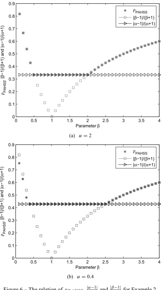
In Figures 3 and 6, we plot the curves of the spectral radius denote byρP A H S S, |α−1|

α+1 and

|β−1_|

β+1 with the change ofβ. From subfigurea, we know thatρP A H S S ≤

|β₋1_|

β+1, asβ ∈ [0.1,0.5],ρP A H S S = |

α₋1_|

α+1, asβ∈ [0.5,2], andρP A H S S ≤ |

β₋1_|

β+1, as β _{∈ [}2,4_], From subfigureb, we know thatρP A H S S ≤ |_ββ₊−1₁|, asβ ∈ [0.1,0.4],

ρP A H S S = |_αα₊−1₁|, as β ∈ [0.4,2.5], and ρP A H S S ≤ |_ββ₊−1₁|, as β ∈ [2.5,4].

Therefore, through the two images, we verify the efficiency and accuracy of Theorem 2.3.

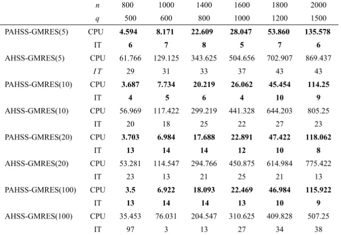
In Tables 3 and 4, by using GMRES(l) (l ₌5,10,20,100) iterative methods with PAHSS preconditioning, we compare between the preconditioner proposed in this paper and the preconditioner in (5) by the iteration numbers (denote by “IT”) and the solution of times in seconds (denote by “CPU”). From the two tables, we can easily see that the superiority of the PAHSS iteration method is very evident.

m 8 12 16 20 24 28 PAHSS-GMRES(5) CPU 0.094 0.625 3.656 14.578 47.563 122.75

IT 7 5 7 8 6 7

AHSS-GMRES(5) CPU 0.250 4.578 31.954 89.234 408.265 886.438

IT 12 22 27 21 36 31

PAHSS-GMRES(10) CPU 0.078 0.485 2.969 12.047 38.313 102.125

IT 10 11 3 5 7 8

AHSS-GMRES(10) CPU 0.094 1.375 11.61 44.094 163 445.39

IT 10 11 11 7 15 12

PAHSS-GMRES(20) CPU 0.078 0.485 2.735 10.765 30.593 77.687

IT 17 11 12 13 13 14

AHSS-GMRES(20) CPU 0.078 0.921 6.453 27.547 89.641 213.891

IT 17 20 10 25 20 20

PAHSS-GMRES(100) CPU 0.078 0.484 2.625 10.50 30.141 76.781

IT 10 11 12 13 13 14

AHSS-GMRES(100) CPU 0.078 0.906 5.016 19.719 67.047 160.328

IT 17 20 22 25 30 30

Table 3 – Example 1: μ₌10,α₌0.5 andβ ₌2.2.

n 800 1000 1400 1600 1800 2000

q 500 600 800 1000 1200 1500

PAHSS-GMRES(5) CPU 4.594 8.171 22.609 28.047 53.860 135.578

IT 6 7 8 5 7 6

AHSS-GMRES(5) CPU 61.766 129.125 343.625 504.656 702.907 869.437

I T 29 31 33 37 43 43

PAHSS-GMRES(10) CPU 3.687 7.734 20.219 26.062 45.454 114.25

IT 4 5 6 4 10 9

AHSS-GMRES(10) CPU 56.969 117.422 299.219 441.328 644.203 805.25

IT 20 18 25 22 27 23

PAHSS-GMRES(20) CPU 3.703 6.984 17.688 22.891 47.422 118.062

IT 13 14 14 12 10 8

AHSS-GMRES(20) CPU 53.281 114.547 294.766 450.875 614.984 775.422

IT 23 13 21 25 21 13

PAHSS-GMRES(100) CPU 3.5 6.922 18.093 22.469 46.984 115.922

IT 13 14 14 13 10 9

AHSS-GMRES(100) CPU 35.453 76.031 204.547 310.625 409.828 507.25

IT 97 3 13 27 34 38

0.35 0.4 0.45 0.5 0.55 0.6 0.65 0.7 −0.2

−0.15 −0.1 −0.05 0 0.05 0.1 0.15 0.2

(a) α=4, β₌2

0.8 1 1.2 1.4 1.6 1.8 2 −0.8

−0.6 −0.4 −0.2 0 0.2 0.4 0.6

(b) α=0.4, β₌0.2

Figure 4 – The distribution of the eigenvalues of_{[ ˜}M(α, β)_]−1A˜for Example 2.

REFERENCES

[1] Z.-Z. Bai, G.H. Golub and M.K. Ng, Hermitian and skew-Hermitian splitting methods for non-Hermitian positive definite linear systems. SIAM J. Matrix. Anal. Appl.,24(2003), 603–626.

[2] M. Benzi and G.H. Golub, A preconditioner for generalized saddle point problems. SIAM J. Matrix Anal. Appl.,26(2004), 20–41.

0.7 0.8 0.9 1 1.1 1.2 1.3 1.4 −1

−0.8 −0.6 −0.4 −0.2 0 0.2 0.4 0.6 0.8 1

(a) α=0.5, β₌2.2

0.4 0.5 0.6 0.7 0.8 0.9 1 1.1 1.2 1.3 −1

−0.8 −0.6 −0.4 −0.2 0 0.2 0.4 0.6 0.8 1

(b) α₌4.5, β₌0.8

Figure 5 – The distribution of the eigenvalues of_{[ ˜}M(α, β)_]−1A˜for Example 2.

[4] Z.-Z. Bai and G.-H. Golub, Accelerated Hermitian and skew-Hermitian splitting iteration methods for saddle point problems. IMA J. Numer. Anal.,27(2007), 1–23.

[5] V. Simoncini and M. Benzi,Spectral properties of the Hermitian and skew-Hermitian splitting preconditioner for saddle point problems.SIAM J. Matrix Anal. Appl.,26(2004), 377–389. [6] Yu.V. Bychenkov,Preconditioning of saddle point problems by the method of Hermitian and

skew-Hermitian splitting iterations.Comput. Math. Math. Phys.,49(2009), 411–421. [7] L.-C. Chan, M.K. Ng and N.-K. Tsing, Spectral analysis for HSS preconditioners.Numer.

0 0.5 1 1.5 2 2.5 3 3.5 4 0 0.1 0.2 0.3 0.4 0.5 0.6 0.7 0.8 0.9 Parameterβ ρP A H S S , | β − 1 |/ ( β + 1 ) a n d | α − 1 |/ ( α + 1 ) ρ PAHSS

|β−1|/(β+1) |α−1|/(α+1)

(a) α=2

0 0.5 1 1.5 2 2.5 3 3.5 4

0 0.1 0.2 0.3 0.4 0.5 0.6 0.7 0.8 0.9 Parameterβ ρ P A H S S , | β − 1 |/ ( β + 1 ) a n d | α − 1 |/ ( α + 1 ) ρ PAHSS

|β−1|/(β+1) |α−1|/(α+1)

(b) α=0.4

[8] T.-Z. Huang, S.-L. Wu, C.-X. Li,The spectral properties of the Hermitian and skew-Hermitian splitting preconditioner for generalized saddle point problems. J. Comput. Appl. Math.,

229(2009), 37–46.

[9] M. Benzi, A generalization of the Hermitian and skew-Hermitian splitting iteration.SIAM J. Matrix Anal. Appl.,31(2009), 360–374.

[10] M. Benzi, M.J. Gander and G.H. Golub,Optimization of the Hermitian and skew-Hermitian splitting iteration for saddle-point problems.BIT,43(2003), 881–900.

[11] Z.-Z. Bai, G.H. Golub and M.K. Ng, On successive-overrelaxation acceleration of the Hermitian and skew-Hermitian splitting iterations.Numer. Linear Algebra Appl.,14(2007), 319–335.

[12] Z.-Z. Bai, G.H. Golub, L.-Z. Lu and J.-F. Yin,Block triangular and skew-Hermitian splitting methods for positive-definite linear systems.SIAM J. Sci. Comput.,26(2005), 844–863. [13] D. Bertaccini, G.H. Golub, S.S. Capizzano and C.T. Possio, Preconditioned HSS methods

for the solution of non-Hermitian positive definite linear systems and applications to the discrete convection-diffusion equation.Numer. Math.,99(2005), 441–484.

[14] Z.-Z. Bai, G.H. Golub and C.K. Li, Optimal parameter in Hermitian and skew-Hermitian splitting method for certain two-by-two block matrices. SIAM J. Sci. Comput.,28(2006), 583–603.

[15] Y.V. Bychenkov,Optimization of the generalized method of Hermitian and skew-Hermitian splitting iterations for solving symmetric saddle-point problems. Comput. Math. Math. Phys.,46(2006), 937–948.

[16] Z.-Z. Bai,Optimal parameters in the HSS-like methods for saddle-point problems.Numer. Linear Algebra Appl.,16(2009), 431–516.

[17] G.H. Golub and C. Greif, On solving block-structured indefinite linear systems.SIAM J. Sci. Comput.,24(2003), 2076–2092.

[18] G.H. Golub and C.F. Van Loan, Matrix Computations. 3rd Edition, The Johns Hopkins University Press, Baltimore (1996).

[19] Z.-Z. Bai, G.H. Golub and C.-K. Li,Convergence properties of preconditioned Hermitian and skew-Hermitian splitting methods for non-Hermitian positive semidefinite matrices. Math. Comput.,76(2007), 287–298.

[20] R.A. Horn and C.R. Johnson, Topics in Matrix Analysis. Cambridge University Press, Cambridge (1991).