Eigenvalues and eigenfunctions of the Laplacian via inverse iteration with shift

(1)

Eigenvalues and eigenfunctions of the Laplacian via inverse iteration

with shift

Rodney Josué Biezuner

a

_{, Grey Ercole}

a,⇑

_{, Breno Loureiro Giacchini}

b

_{, Eder Marinho Martins}

c

a_{Departamento de Matemática-ICEx, Universidade Federal de Minas Gerais, Av. Antônio Carlos 6627, Caixa Postal 702, 30161-970 Belo Horizonte, MG, Brazil}

b_{Departamento de Física-ICEx, Universidade Federal de Minas Gerais, Av. Antônio Carlos 6627, 31270-901 Belo Horizonte, MG, Brazil} c

Departamento de Matemática-ICEB, Universidade Federal de Ouro Preto, Campus Universitário Morro do Cruzeiro, 35400-000 Ouro Preto, MG, Brazil

a r t i c l e

i n f o

Keywords:

Laplacian Eigenvalues Eigenfunctions Fourier series

Inverse iteration with shift Rayleigh quotient

a b s t r a c t

In this paper we present an iterative method, inspired by the inverse iteration with shift technique of finite linear algebra, designed to find the eigenvalues and eigenfunctions of the Laplacian with homogeneous Dirichlet boundary condition for arbitrary bounded domainsXRN. This method, which has a direct functional analysis approach, does not approximate the eigenvalues of the Laplacian as those of a finite linear operator. It is based on the uniform convergence away from nodal surfaces and can produce a simple and fast algorithm for computing the eigenvalues with minimal computational requirements, instead of using the ubiquitous Rayleigh quotient of finite linear algebra. Also, an alterna-tive expression for the Rayleigh quotient in the associated infinite dimensional Sobolev space which avoids the integration of gradients is introduced and shown to be more effi-cient. The method can also be used in order to produce the spectral decomposition of any given functionu2L2_ðXÞ.

1. Introduction

In [1] we introduced an iterative method for computing the first eigenpair of the p-Laplacian operator

Dpu:¼div jrujp2ru

; p>1, with homogeneous Dirichlet boundary condition in a bounded domainXRN; NP1. The

technique was inspired by the inverse power method or inverse iteration of finite linear algebra.

In the present paper we concentrate in the special casep¼2, the Laplace operatorD, which was superficially dealt with in

[1]. Besides clarifying some of the arguments sketched in that paper for this case and providing some error estimates, our

main purpose in this work is to show how inverse iteration with shift in the presence of uniform convergence can be used in order to obtain a fast and efficient method for computing the eigenvalues and eigenfunctions of the Laplacian operator

with homogeneous Dirichlet boundary condition for any bounded domainX. If the eigenvalues or at least good estimates

for them area prioriknown, the method can produce the corresponding eigenfunctions with great speed and accuracy.

The technique can alternatively also be used as a fast process to obtain the spectral decomposition of any function

u2L2_ð_X_Þ_{(in other words, the Fourier series of}_u_).

We remark that the application of the method to the special case of the Laplacian operator is more natural since the

Lapla-cian is a linear operator,L2ðXÞis a Hilbert space and the inverse operatorD1is a self-adjoint and compact operator,

there-fore allowing the complete characterization of its spectral structure, as well as having the property that its eigenfunctions

constitute a basis forL2ðXÞ(except for compactness, these properties are absent in thep-Laplacian whenp–2).

http://dx.doi.org/10.1016/j.amc.2012.06.025

⇑ Corresponding author.

E-mail addresses:rodney@mat.ufmg.br(R.J. Biezuner),grey@mat.ufmg.br(G. Ercole),brenolg@ufmg.br(B.L. Giacchini),eder@iceb.ufop.br(E.M. Martins). Contents lists available atSciVerse ScienceDirect

Applied Mathematics and Computation

(2)

Our approach of the inverse iteration with shift is based on the following iterative process started by a given function

u2L2ðXÞ:

/0:¼u and

D

r

/nþ1¼/n in

X

; /nþ1¼0 on@

X

;

ð1Þ

where

r

>0 is a previously fixedshiftandDr:¼Dþ

r

Iis the correspondingshifted operator.

The sequencef/ngis then handled in order to produce approximations for the pairðkru;eruÞwherekrudenotes the

eigen-value of the Laplacian appearing in the spectral expansion ofuwhich is closest to

r, and

er

udenotes the eigenfunction

ob-tained as the projection ofuon thekru-eingenspace.

Inverse iteration with shift is used in finite linear algebra in order to find the eigenvalues and eigenfunctions of a

finite-dimensional linear operator. As an eigenvalue-finding procedure it is not as efficient as other methods, such as theQR

algo-rithm. However, if very good estimates of the eigenvalues are known in advance, its rate of convergence to both eigenvalues

and eigenfunctions can be very fast (see[2], for instance).

This approach can be naturally extended to self-adjoint compact linear operators in infinite-dimensional Hilbert spaces such as the Laplacian and those arising in Sturm–Liouville problems. In spite of this, we have not been able to find any ref-erence in the literature to this approach being used in the Laplacian context.

Since there is now a vast literature concerning the search for estimates for the eigenvalues of the Laplacian, as well as the

gaps between eigenvalues (see, for instance,[3–6]; although particularly useful in our context would be lower bounds for the

difference between consecutive eigenvalues), these results can be used in connection with the inverse iteration with shift algorithm to find eigenfunctions of the Laplacian in arbitrary domains, as well as better approximations for its eigenvalues. It must be emphasized, however, that as with the finite linear method, the inverse iteration with shift method is not capable to find all the eigenfunctions associated to a non-simple eigenvalue. It can only find an eigenfunction of the associated

eigen-space. In the generic sense most domains have Laplacian spectra consisting only of simple eigenvalues (see[7,8]), although

many domains of practical interest have eigenvalues with multiplicity greater than one (usually, domains which exhibit some type of symmetry, although not all of them).

Algorithm 1 below is the simplest version of the inverse iteration with shift algorithm for computing one specific eigen-value and corresponding eigenfunction of the Laplacian.

Algorithm 1:Inverse iteration with shift for Laplacian eigenvalue and eigenfunction

1:/0¼u

2: Setx0 (point inXoutside nodal surfaces, randomly chosen)

3: Set

r

(shift, usually eigenvalue estimate)

4: Setm (number of iterations, depending on method used to solve Laplacian)

5:forn¼0;1;2;. . .;mdo

6: SolveDr/nþ1¼/ninX; /nþ1¼0 on@X

7:end for

8:return/_mþ1= /mþ1

1 (L

1_{-normalized eigenfunction)}

9:return/mðx0Þ=/mþ1ðx0Þ þ

r

ðeigenvalueÞ

In principle, the functionuat the start of Algorithm 1 should be chosen so that it will have components in all eigenspaces

of the Laplacian and a random choice would suffice. However, in practice, due to rounding errors any simple function can be

used. In our numerical tests (see Section6), we observed that even the unit constant function could be used in order to obtain

all the eigenvalues, even in a domain where it does not have an infinite number of them in its spectral decomposition. In Line 6 of Algorithm 1 any PDE solver can be used. This allows one to choose the fastest solver available for a particular

domain. In Line 9 the eigenvalue is computed according to the uniform convergence theory developed in Section4. Since

uniform convergence occurs away from nodal surfaces, a pointx02Xnot in a nodal surface must be chosen; because nodal

surfaces have zeroN-dimensional measures, a random choice will suffice in the vast majority of cases, even taking into

ac-count that nodal surfaces change as the computed eigenfunction changes.

In finite linear algebra, the approximation to the eigenvalue is usually computed using the Rayleigh quotient. In our con-text, the eigenvalue can also be computed via the Rayleigh quotient of the approximated eigenfunction:

R/nþ1

¼

r

/nþ1;

r

/nþ1

2 /nþ1;/nþ1

2

¼

r

/nþ1

2 2 /nþ1

2 2

¼

R

X

r

/nþ1

2 dx

R

X/ 2 nþ1dx

: ð2Þ

However, due to the high oscillatory nature of high frequency eigenfunctions, in order to accurately compute the integral of the (squared) gradient of eigenfunctions associated with these eigenvalues, a much finer grid needs to be used, which

af-fects the efficiency of the method. Therefore, the Rayleigh quotient in its original form(2)is not recommended for the

com-putation of the eigenvalues of the Laplacian, unless one is prepared to incur the higher comcom-putational costs (see also further

(3)

Nonetheless, an integration by parts argument produces the following alternative expression for the Rayleigh quotient that avoids computations involving gradients:

Rð/nÞ ¼

r

þ

R

X/n/n1dx

R

Xj/nj

2_dx : ð3Þ

We obtain very satisfactory results by using this sequence in Line 9 of Algorithm 1 to compute eingenvalues in our

numerical tests (see Section6).

Another alternative way to compute the eigenvalues is given by the quotient

k/nk2 k/nþ1k2

þ

r

¼

R

X/ 2 ndx

R

X/ 2 nþ1dx

þ

r

; ð4Þ

when the shift

r

is chosen below the eigenvalue. This quotient also gives accurate approximations for the eigenvalues even

using relatively coarse meshes; the computation of the integrals of the approximated eigenfunctions, instead of their

gradi-ents, does not appear to be significantly affected by the use of coarse grids (see Section6).

We believe that, differently from what happens in finite dimensions, where much better and faster algorithms for finding the eigenvalues of linear operators (matrices), specially self-adjoint operators, are available, the inverse iteration with shift algorithm can be a very competitive method for finding the eigenvalues of the Laplacian. Typical algorithms for computing Laplacian eigenvalues involve the discretization of the Laplacian operator and the computation of the eigenvalues of the resulting discretization matrix. However, since only a small number of the eigenvalues of the discretization matrix are good approximations to the Laplacian eigenvalues (the smaller ones), huge matrices are necessary in order to obtain a sufficiently good number of eigenvalues. And some problems, particularly those arising in the study of quantum billiards, demand the computation of a very large number of eigenvalues. Needless to say, besides the requirements of memory, the size of the

matrix makes it computationally costly to find its eigenvalues (see the classical[9]book, the review[3]and the more recent

work[10]for details).

The inverse iteration with shift method, that requires only typical relatively modest sizes for meshes in order to solve the Poisson equation with homogeneous Dirichlet boundary condition, can be very competitive in terms of memory allocation and processing time. This is true even when one considers that in order to find accurate approximations for the highest order eigenvalues and eigenfunctions sometimes one needs to refine the mesh, due to the increase of oscillations.

Even if good estimates for the eigenvalues of a particular domain are not known in advance, a few iterations of inverse iteration with shift should be able to find good approximations to them, which can work as first estimates for the shift on a second run of the algorithm. The first choices for the shift might be concentrated around the numbers given by Weiyl’s Law

(see[11]or[12]).

The inverse iteration with shift method can also be used in order to find the spectral decomposition of any function

u2L2ð ÞX, that is, in order to find its projections on the Laplacian eigenspaces. One has only to be careful to eliminate

spu-rious projections, that is, projections which arise from rounding errors. This can be done through computing the Fourier coef-ficient associated to each eigenspace. If this coefcoef-ficient becomes less than a specified very small tolerance, this projection can be safely discarded as arising from rounding errors. The two algorithms can be combined together in order to simultaneously find both the desired spectral decomposition of a given function defined on a domain and the spectrum of the Laplacian on it.

The spectral decomposition algorithm is given below (Algorithm 2). Once again, Line 11 can be replaced by(3)or(4).

Algorithm 2:Spectral decomposition

1:/0¼u

2: Setx0 (point inXrandomly chosen)

3:fork¼0;1;2;. . .do

4: Setrk ðshiftÞ

5: forn¼0;1;2;. . .do

6: SolveDrk/

k

nþ1¼/kninX; /knþ1¼0 on@X

7: Compute u;/k_nþ1= /knþ1

₂

D E

2 (Fourier coeficient)

8: if u;/k_nþ1= /knþ1

₂

D E

2

>tolerancethen

9: return/k_nþ1= /knþ1

₂ (L

2_{-normalized eigenfunction)}

10: return u;/k_n_þ₁=/k_n_þ₁

₂

D E

2 (Fourier coefficient)

11: return/_nðx0Þ=/nþ1ðx0Þ þ

r

k ðeigenvalueÞ break

(4)

Although for the sake of simplicity all computations here are done for the Laplacian, the same algorithm can be used for similar elliptic operators.

This paper is organized as follows. The inverse iteration with shift sequence is defined in Section2, where most of the

notation used in this paper is also established. In Section3 some well-known results concerning the Rayleigh quotient

are recalled and proven for completeness. In Sections3 and 4we discussL2and uniform convergence of the inverse iterated

sequence, respectively. In the short Section5we make some considerations about the normalization process on each step of

(1)which is useful for computational purposes, and in Section6we present the results of some numerical experiments made

in simple domains.

Finally, in Section7we discuss if the rate of convergence of the method could theoretically be improved through the use

of the inverse iteration with shift given by the Rayleigh quotient, as it is standard practice in finite linear algebra.

2. Definition of the inverse iteration with shift sequence

LetXbe a bounded domain inRNandH ¼f gek 1k¼1H10ð ÞX be an orthogonal (not necessarily normalized) basis forL2ð ÞX

consisting of eigenfunctions of the Laplacian operator with homogeneous Dirichlet boundary condition, that is,

D

ek¼kkek in

X

; ek¼0 on@

X

;

wheref gkk 1k¼1is the non-decreasing sequence of eigenvalues of the Laplacian, counting multiplicities:

0<k1<k26. . . ð5Þ

Let

r

>0 and define theshifted operator

D

r:¼

D

þ

r

I: ð6Þ

It follows thatekis also an eigenfunction ofDrcorresponding to the eigenvaluekk

r.

Conversely, ifkis an eigenvalue ofDr, thenk¼kk

r

for somek. Thus, the spectrum of the shifted operator equals the

spectrum of the Laplacian operator shifted to the left by

r, while the corresponding eigenspaces are the same.

Givenu2L2ð ÞX, let

u¼X

1

k¼1

ak

ek

be the Fourier expansion ofu, so that the Fourier coefficients

a

kare given by

ak

¼hu;eki2 ek k k22

¼

R

Xuekdx

R

Xe 2 kdx

:

Denote byk1_uthe least eigenvalue whose associated eigenspace is not orthogonal tou. That is,

k1u:¼kk1 where k1¼minfk:

ak

–0g:

In other words,k1_uis the first eigenvalue such thatuhas a non-zero component in the corresponding eigenspace. Note that

ifr1is the multiplicity ofkk1then

k1u¼kk1¼kk1þ1¼ ¼kk1þr11:

We will denote bye1

uthe orthogonal projection ofuon thek

1

u-eigenspace, that is

e1

u:¼

ak

1ek1þ

ak

1þ1ek1þ1þ þ

ak

1þr11ek1þr11¼ X

kk¼k1u

ak

ek:

Thus, the Fourier expansion ofucan be rewritten as

u¼ X kkPk1u

ak

ek¼e1uþ

X

kk>k1u

ak

ek¼e1uþ

X

kPk1þr1

ak

ek:

Proceeding in this way, denoting byej

uthe orthogonal projection ofuon thekju-eigenspace which is thejth-eigenspace not

orthogonal tou, the eigenfunction expansion ofucan be written in terms of its non-zero components in the eigenspaces of

the Laplacian as

u¼X M

j¼1 ej

u; ð7Þ

where eitherMis a positive integer or, as in most cases,M¼ 1, and the corresponding sequence of eigenvalues kju

n o1

j¼1is (strictly) increasing

(5)

As is well known from the theory of compact linear operators, if

r

does not belong to the spectrum ofDwe have that

ðDrÞ1:L2ð Þ !X L2ð ÞX is a continuous, compact and invertible operator. Therefore, whenever

r

is not an eigenvalue of the

Laplacian, we can define a sequencef/ngn2NH

1

0ð ÞX by inverse iteration setting

/0¼u and

D

r/nþ1¼/n in

X

; /nþ1¼0 on@

X

:

ð8Þ

For eachu2L2ð ÞX and

r

>0 not in the Laplacian spectrum consider the sequencef/ngdefined by inverse iteration in(8).

Since/nþ1¼ ð DrÞ1/n, it follows from(7)that the eigenfunction expansion of/nis given by

/n¼

X

M

j¼1 1

kju

r

ne

j u:

Letkrube the Laplacian eigenvalue appearing in the spectral decomposition ofuwhich is closest to

r, i.e.,

kru

r

¼min

j2N k j u

r

: ð9Þ

Now leter

udenote the projection ofuon thekru-eigenspace. Then

u;er

u

2¼ e

r

u;eru

2¼ e

r

u

2

2 ð10Þ

and we can write

/n¼ 1

kru

r

ne r

uþ

X

M

kjur j j>jkrurj

1 ðkju

rÞ

ne j u¼

1

kru

r

n e

r

uþ

X

M

kjur j j>jkrurj

kru

r

kj

r

n

ej u

0

B @

1

C A;

or

/n¼ 1

kru

r

n e r

uþwn

; ð11Þ

where

wn¼

X

M

kjur j j>jkrurj

kru

r

kju

r

!n

ej

u: ð12Þ

Throughout this paper, we will denote byksuthe Laplacian eigenvalue appearing in the spectral decomposition ofuwhich

is second closest to

r, i.e.,

ksu

r

¼ min

j2N

kju–k

r

u kju

r

: ð13Þ

We will also denote byunthe component ofuin the direction ofk//nnk2, that is:

un:¼ u; /n

/n

k k2

2 /n /n

k k2¼

Z

X u /n

/n k k2dx

/n /n

k k2: ð14Þ

3.L2-convergence of inverse iteration with shift

In this section we expose theL2-approach of the inverse iteration with shift. Firstly let us state some well-known results

concerning the Rayleigh quotientR:H10ð Þ nX f g !0 Rdefined by

Rð

v

Þ ¼

R

Xj

r

v

j 2_dx

R

X

v

2dx

: ð15Þ

For ease of consultation, we give short proofs of these results.

Proposition 1. A function u2H10ð Þ nX f g0 is a critical point ofRif and only if u is an eigenfunction of the Laplacian with

homogeneous Dirichlet boundary condition andRð Þu is the corresponding eigenvalue.

Proof.Given

v

₂H1₀ð ÞX, we have

R0_ð_u_Þ

_v

_¼ 2

u k k22

r

u;

r

v

h i2 Rð Þu_hu;

v

_i2

(6)

Therefore,R0_{ð Þ ¼}_u _{0 if and only if}

Z

X

r

u

r

v

¼ Rð Þu

Z

X u

v

for all

v

₂W1₀;2_{ð Þ}_X, that is,uis a weak solution of

D

u¼ Rð Þuu in

X

; u¼0 on@

X

:

Corollary 2. The Rayleigh quotient gives a quadratically accurate estimate for the Dirichlet Laplacian eigenvalues, that is, if u is an eigenfunction of the Laplacian with homogeneous Dirichlet boundary condition withRð Þu as the corresponding eigenvalue, then

Rð Þ R

v

ð Þ ¼u O k

v

uk2

as

v

_!u in L2_ð_X_Þ.

Proof. If follows immediately from Taylor’s formula, sinceR0_{ð Þ ¼}_u _0.

h

Now we give the main result of this section. Before this, we note from(11)of Section2that

/n /n k k2

¼ e

r

uþwn er

uþwn

₂

; ð16Þ

where the sign of the right-hand side will depend on whether the shift

r

is taken above or below the eigenvalue. With

re-spect ton: if the shift is taken below the eigenvalue, the sign will always be positive, whereas if the shift is chosen above the

eigenvalue the sign will beð1Þn.

We note from(14) and (16)that

un¼ u; er

uþwn er

uþwn

₂

* +

2 er

uþwn er

uþwn

₂

ð17Þ

and also remark that

Rð/nÞ ¼

r

þ

R

X/n/n1dx

R

Xj/nj

2_dx : ð18Þ

This fact follows from an integration by parts after multiplying the equationDr/n¼/n1by/n. From the computational

viewpoint,(18)has the advantage of avoiding the computation of the gradientr/nas required in(15).

Theorem 3. Let u2L2ð ÞX.

(i)We have

wn

k k26 k

r

u

r

ksu

r

n u k k2:

In particular,wn!0in L2ð ÞX with an exponential rate.

(ii)There exists n02Nsuch that er

uþwn er

uþwn

₂

e

r

u er

u

₂

6 4 er

u

₂

wn

k k2

for all nPn₀.In particular,

er

uþwn er

uþwn

₂

! e

r

u er

u

₂

in L2ð Þ

X

; ; ð19Þ

with an exponential rate.

(iii)The following convergences hold:

/n k k2 /nþ1

₂

! kru

r

; ð20Þ

un!eru in L 2

X

(7)

where unis defined by(14),and

Rð/nÞ !k

r

u; ð22Þ

with

Rð/nÞ kru¼O

kru

r

ksu

r

2n!

: ð23Þ

Proof.We have from(12)that

wn k k22¼

X

M

kjur j j>jkrurj

kru

r

kju

r

2n ej u 2 26

kru

r

ksu

r

2n X M

kjur j j>jkrurj

ej u 2 26

kru

r

ksu

r

2n u k k22:

Since

kru

r

ksu

r

< 1;

it follows thatkwnk2!0 asn! 1, which proves(i).

Letn02Nbe such that

wn k k26

1 2 e r u

for allnPn0:

Thus, ifnPn₀it follows that

1 2 e r u ₂¼ er_u

₂ 1 2 e r u

₂6 er_uþwn

₂þkwnk2kwnk2¼ eruþwn

₂ and er

uþwn er

uþwn

₂ e r u er u ₂ ₂ ¼ e r u

₂ er_uþwn

er

u eruþwn

₂

er

uþwn

₂ er_u

₂ ₂ 6 er

u eru

₂ eruþwn

₂

þ er

u

₂wn 1=2

ð Þ er

u 2 2 ₂

62 e

r

u

₂kwnk2þ eru

₂kwnk2 er u 2 2 ¼ 4 er u ₂ wn k k2;

which proves (ii). Since

/n k k2 /nþ1

₂

¼ kru

r

er

uþwn

₂

er

uþwnþ1

₂

;

(20)follows from(i).

TheL2-convergence(21)follows from(17), (19)and(10).

In order to prove(22)we firstly notice that

lim /n1

/n1

k k2;

/n /n k k2 2 ¼ e r u er u ₂ ; e r u er u ₂ * + 2 1 1

ifkruP

r

; ifkru<

r

:

In fact, ifkruP

r

then

lim /n1

/n1

k k2;

/n /n

k k2

2

¼lim eruþwn1 er

uþwn1

₂ ; e r

uþwn er

uþwn

₂ * + 2 ¼ e r u er u ₂ ; e r u er u ₂ * + 2 ;

while ifkru<

r

then

lim /n1

/n1

k k2

; /n /n k k2

2

¼lim ð1Þn1 e

r

uþwn1 er

uþwn1

₂

;ð1Þn e

r

uþwn er

uþwn

₂ * + 2

¼ e

r u er u ₂ ; e r u er u ₂ * + 2 :

Thus, it follows from(18)that

limRð/nÞ ¼

r

þ k

r

u

r

1 1

if kruP

r

; if kru<

r

:

(8)

The convergence order(23)follows from(21)andCorollary 2, since

Rð/nÞ kru¼ Rð Þ Run eru

¼O uneru

2 2

¼O k

r

u

r

ksu

r

2n!

:

4. Uniform convergence of inverse iteration with shift

We begin this section by stating aL1_{-estimate for an eigenfunction of the Laplacian in terms of its}_L2_{-norm. In the}

fol-lowing, we denote byj jX the Lebesgue measure ofX.

Lemma 4. Let e2H1₀ð ÞX be an eigenfunction ofDcorresponding to the eigenvaluek. Then

e k k164

N

X

j j1=2kN=2k k2e : ð24Þ

Proof. It is shown in[13], without any smoothness assumption on@X, that ifeis an eigenfunction corresponding to a

var-iational eigenvaluekof the homogeneous Dirichlet problem for thep-Laplacian then

e k k164

N

kN=pk ke L1ð ÞX:

Choosingp¼2,(24)follows from Hölder’s inequality. h

Estimates for eigenfunctions of the Laplacian with the exponentN=2 in the eigenvalue replaced byN=4 can be found in

[14–17]. See also[18, Remark 5.21]for more references.

The following result refers to the nondecreasing sequence(5)of eigenvalues of the Laplacian.

Lemma 5. If k>N=2, then

X1

j¼1 1

kkj 6 NC

k

2kN<1; ð25Þ

where C is a positive constant which depends only on N andj jX.

Proof. It is well known (see[19,20]) that

kjP1 Cj

2=N ;

where

C¼Nþ2 N

xN

j j

X

ð Þ2=N

4

p

2 ð26Þ

and

x

Nis the volume of theN-dimensional unit ball. Hence, ifj>N=2 we have

X1

j¼1 kjk6C

kX1

j¼1 j2k=N

<CkZ 1 1

s2k=N_ds_¼ NC k

2kN:

In the next lemma we show that the convergence of a series formed by the eigenvalueskjuwhich appear in the spectral

decomposition of a functionu2L2ð ÞX follows from the convergence of a series formed by all eigenvalues of the Laplacian.

Lemma 6. Let k be chosen so that the seriesP1

j¼1_k1k j

is convergent. Then the series

X

M

j¼1 kju

N=2

kju

r

N=2þkþ1

is also convergent.

Proof. Assume that the expansion ofuis not finite, i.e.,M¼ 1(otherwise the result is trivial). Since

X1

j¼1 1

kju

k

6X

1

j¼1 1

(9)

it suffices to show that

kju

N=2

kju

r

N=2þkþ16 1

kju

k ð27Þ

for all sufficiently largej.

Askj_u! 1, there existsj0such that kju

r

¼k j

u

r

for alljPj0. Thus, ifjis sufficiently large, we can write

kju

N=2þk

kju

r

N=2þk¼ kju

N=2þk

kju

r

N=2þk<k

j

u

r

¼ k j u

r

;

whence(27)follows. h

In order to prove the uniform convergence of the inverse iteration sequencef/ngn2N, we return to(11)and write

/n /n k k1

¼ e

r

uþwn er

uþwn

1

: ð28Þ

As in(16), the sign of the right-hand side will depend on whether the shift is taken above or below the eigenvalue and onn.

Lemma 7. The inequality

wn k k16K

kru

r

ksu

r

nh

ð29Þ

holds for all sufficiently large n, for someh>0and a positive constant K¼K u;X; kru

r

. In particular,wn!0uniformly inX with an exponential rate.

Proof.From(12)and Lemma4we obtain

wn

j j6 X

M

kjur j j>jkrurj

kru

r

kju

r

n ej u 64 N

X

j j1=2k ku 2

X

M

kjur j j>jkrurj

kru

r

kju

r

n

kju

N=2

:

But, takingh¼N=2þkþ1, we have

X

M

kjur j j>jkrurj

kru

r

kju

r

n

kju

N=2

¼ kru

r

h X M

kjur j j>jkrurj

kru

r

kju

r

nh kju

N=2

kju

r

h6 k

r

u

r

hkru

r

ksu

r

nh

X

M

kjur j j>jkrurj

kju

N=2

kju

r

h 6 k r

u

r

ksu

r

nh kru

r

hX M

j¼1 kju

N=2

kju

r

h

and by Lemma6the last series converges. Thus,(29)follows if we take

K¼4N

X

j j1=2k k2u kru

r

hX M

j¼1 kju

N=2

kju

r

h:

Theorem 8. Let u2L2ð ÞX. Then

(i) There exists n02Nsuch that er

uþwn er

uþwn

₁ e r u er u ₁ 1 6 4 er u ₁ wn k k1

(10)

er

uþwn er

uþwn

1 ! e r u er u 1

uniformly in

X

with an exponential rate.

(ii) The following convergences hold

/n k k1

/nþ1

1

! kru

r

ð30Þ

and

un!eru uniformly in

X

: ð31Þ

(iii) IfK x:eruðxÞ–0

is compact, then /n

/nþ1!k

r

u

r

uniformly and with an exponential rate.

Proof. Letn0be such thatkwnk1612 eru

1for allnPn0. Then, as in the proof of(ii)ofTheorem 3, we have for allnPn0that

1 2 e r u

₁6 eruþwn

₁ and er

uþwn er

uþwn

1 e r u er u 1 1 6 4 er u 1 wn k k1:

The remaining of(i)follows fromLemma 7.

In order to prove(31), write

un¼ /n k k1

/n

k k2

2

/n /n k k1

Z

X u /n

/n k k1

dx:

Since

limk/nk1

/n k k2

¼lim e r

uþwn

1 er

uþwn

₂ ¼ e r u 1 er u ₂

and, from(i),

/n /n k k1

Z

X u /n

/n k k1

dx! e

r u er u 1 Z X u e r u er u 1 dx

uniformly inX, it follows from(10)that

un! er u ₁ er u ₂ !2 er u er u 1 Z X u e r u er u 1

dx¼ e

r u er u 2 2 Z X uer

udx¼ er u er u 2 2

u;er

u

¼er

u:

Since from(11)we have

/n k k1

/nþ1

1

¼ kru

r

er

uþwn

1 er

uþwnþ1

1

and thus(30)also follows fromLemma 7.

Now, letK supper

u be compact so that

m:¼min

K e r u >0

and fixn02Nsuch that

wn k k1<

m

2 for allnPn0:

Thus ifnPn₀we have onK

er

uþwn

P er_u

jw_njPmkw_nk₁>

m

2:

(11)

/n /nþ1

¼ kru

r

e

r

uþwn er

uþwnþ1

makes sense onKfor all sufficiently largenand again(iii)follows fromLemma 7since

/n /nþ1

kru

r

¼

kru

r

er

uþwn er

uþwnþ1

1

¼

kru

r

wnwnþ1 er

uþwnþ1

62k

r

u

r

m wnwnþ1

:

5. Normalization at each step

In order to avoid numerical problems, such as overflow or underflow, it is usual to normalize the right-hand-side function in each inverse iteration. Although this procedure changes the sequence of iterates it maintains convergences.

In fact, let

v

_nbe defined by

v

₀¼ u u

k k and

D

r

v

_n_þ₁_¼ vn vn

k k in

X

;

v

_n_þ₁_¼0 on_@

X

_:

(

ð32Þ

wherek k may denote theL2-norm or theL1_{-norm. Then, since}

_r

_{is not an eigenvalue of}

Dit is easy to verify that

/nþ1¼k/nk

v

nþ1: ð33Þ

Hence, for example, if one usesk k ¼ k k2then

u;

v

n

v

_n

k k2

2

v

_n

v

_n

k k2¼un!e

r

u; ð34Þ

both uniformly and inL2. Note that this sequence is exactly the sequencefungdefined by(14)and rewritten in terms of the

sequence_f

v

_n_g.

Moreover, in view of(33) and (15)one also has

Rð

v

nÞ ¼ Rð/nÞ !kr_u: ð35Þ

Ifk k ¼ k k1then one has the following uniform convergence in each compactK x:eruðxÞ–0

:

v

_n

v

_n_þ₁! kru

r

kru

r

¼ 1

1

if kru>

r

; if kru<

r

:

6. Numerical tests

In this section we present some numerical tests on the unit interval, unit disk and unit square. The inverse iteration with

shift was implemented starting from the unit constant functionu1 on these domains. Eigenvalue approximations were

computed by running our Algorithm 1 and taking (in the line 9) the following sequences considered in this paper:

l

n:¼ /n /nþ1

ðx0Þ þ

r

;

cn

:¼ k/nk2

k/nþ1k2

þ

r

and

Rð/nÞ ¼

r

þh/n;/n1i2 /n k k22

: ð36Þ

This last sequence is an alternative form of the Rayleigh quotient evaluated at/naccording to(18). As previously remarked,

the numerical advantage of writing the Rayleigh quotient in this form is that one need not compute the gradientr/n.

Taking into account(35)we also compute eigenvalue approximations using the sequenceRð

v

nÞwhere

v

nis defined by

(32). Namely, we use the following alternative expression for this sequence:

Rð

v

nÞ ¼

r

þ

v

_n_;

v

_n₁

h i2

v

_n k k22

: ð37Þ

Notwithstanding the (theoretical) equalityRð

v

_n_{Þ ¼ Rð}/nÞ, our tests indicate some remarkable numerical differences

be-tween them.

The non-normalization of the function/non each step in Algorithm 1 tends to attribute to it smaller values at each

iter-ation. Thus, as a numerical phenomenon, the quotient/n=/nþ1tends to assume the value 1, what makes the sequences

l

n;

c

nandRð/nÞconverge to

r

þ1.

(12)

On the other hand, the sequenceRð

v

_n_Þseems to be more robust, since we did not observe this phenomenon when using

it. Another indication of its numerical stability is its tendency to better capture the correct eigenvalues (i. e. those belonging to the spectrum of the starting function), than the other sequences.

The graphs of the eigenfunction approximations were constructed by using the sequenceunin(34). In Algorithm 2, these

approximations can be viewed as the combination of lines 9 and 10 with/knþ1replaced by

v

knþ1(normalizing on each step).

To show the efficiency of inverse iteration with shift we used neither the most efficient available method for solving the underlying differential equation nor a fine grid, but one of the most basic methods, finite differences, and a relatively coarse grid. Integrals were computed via the Simpson composite method.

6.1. Eigenvalues and eigenfunctions for the unit interval½0;1

In this case,(8)becomes the following boundary value problem

/00nþ1

r

/nþ1¼/n; /nþ1ð0Þ ¼/nþ1ð1Þ ¼0: (

One can verify thatkk¼k2

p

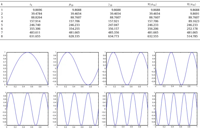
2and that the functionu1 does not have components corresponding tokkforkeven.

We present inTable 1exact and approximated eigenvalues of the Laplacian on the unit interval. The shift was set to the

corresponding exact eigenvalue minus 0.1 (that is,

r

k:¼kk0:1), and a grid of only 101 nodes was used. As shown in the

last column, the sequenceRð

v

_n_Þseems to capture only the eigenvalueskr_uthat appear on the spectral decomposition of the

Table 1

Exact and approximated eigenvalues on the unit interval½0;1obtained from the inverse iteration with shift starting from the unit function. The shift rk:¼kk0:1 and a grid containing 101 nodes were used.

k kk l10 c10 Rð/10Þ Rðv₁₀_Þ

1 9.8696 9.8688 9.8688 9.8688 9.8688

2 39.4784 39.4654 39.4654 39.4654 9.8691

3 88.8264 88.7607 88.7607 88.7607 88.7607

4 157.914 157.706 157.921 157.706 89.1623

5 246.740 246.233 247.047 246.233 246.233

6 355.306 354.255 356.157 356.206 252.178

7 483.611 481.665 485.356 481.665 481.665

8 631.655 628.335 634.773 632.555 514.785

0 0.2 0.4 0.6 0.8 1 0

0.1 0.2 0.3 0.4 0.5 0.6 0.7 0.8 0.9 1

0 0.2 0.4 0.6 0.8 1 −1

−0.8 −0.6 −0.4 −0.2 0 0.2 0.4 0.6 0.8 1

0 0.2 0.4 0.6 0.8 1 −1

−0.8 −0.6 −0.4 −0.2 0 0.2 0.4 0.6 0.8 1

0 0.2 0.4 0.6 0.8 1 −1

−0.8 −0.6 −0.4 −0.2 0 0.2 0.4 0.6 0.8 1

0 0.2 0.4 0.6 0.8 1 −1

−0.8 −0.6 −0.4 −0.2 0 0.2 0.4 0.6 0.8 1

0 0.2 0.4 0.6 0.8 1 −1

−0.8 −0.6 −0.4 −0.2 0 0.2 0.4 0.6 0.8 1

0 0.2 0.4 0.6 0.8 1 −1

−0.8 −0.6 −0.4 −0.2 0 0.2 0.4 0.6 0.8 1

0 0.2 0.4 0.6 0.8 1 −1

−0.8 −0.6 −0.4 −0.2 0 0.2 0.4 0.6 0.8 1

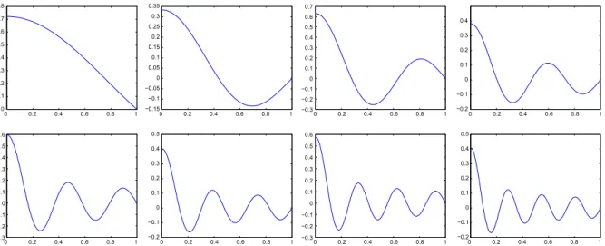
Fig. 1.First eight approximated eigenfunctions of the Laplacian on½0;1obtained from the inverse iteration with shift starting from the unit function.

Table 2

NumberNkof approximates with relative error of orderforrk:¼0:99kk, grid containing 10,001 points and 30 iterations.

103 ₁₀4 ₁₀5 ₁₀6 ₁₀7 ₆₁₀8

(13)

functionu1. In fact, we note that for even values ofkthe shift is closer tokkthankk1and even so the corresponding

se-quenceRð

v

_nÞconverges tokk1which is the correct eigenvalue.

InFig. 1we present the graphs of the first eight approximated eigenfunctions.

Table 1also exemplifies the numerical convergence to

r

þ1 of the non-normalized sequenceRð/nÞ, which happened to

the approximations ofk6andk8. For the first one, for example, the closest approximation achieved isRð/4Þ ¼280:278. For

n>4 the quotient collapses to one and the result is spurious. In order to compute a correct approximation of this eigenvalue

using this sequence, a finer grid should be used.

InTable 2we show the result of calculating the first 1,500 eigenvalues of the unit interval using the normalized sequence

Rð

v

_nÞwith 30 iterations and a grid containing 10,001 nodes. The relative error between the computed eigenvalueRð

v

_nÞand

the exact eigenvaluekis defined by

ðRð

v

_nÞ_;_k_{Þ ¼} Rð

v

nÞ _k

k

:

The shift used to makeTable 2is

r

k:¼0:99kk, which has an initial relative error of 1%. Such error is huge for great

eigen-values and the intervalð

r

k;kkÞmay contain many other eigenvalues. Thus, it is likely to happen that this shift makes the

sequence converge to an eigenvaluekrdifferent fromkk. With this in mind, we considered thatRð

v

₃₀Þcorrectly

approxi-mated an eigenvaluekrif_jkr Rð

v

₃₀_Þ_{j ¼}min_s_jks Rð

v

₃₀_Þ_j, and that_Rð

v

₃₀_Þconverged tokrif their relative error is less than

103_.

Table 2reveals that among the 1,500 shifts used, all of them approximated an eigenvalue with a relative error of order of

magnitude 103_{, and that 1,208 converged with a relative error less than 10}3_.

Among the 1,208 converged approximations, 547 refer to eigenvalueskkwithkeven. This shows that the sequenceRð

v

_n_Þ

can converge to an eigenvalue that does not belong to the spectrum of the unit function.

In order to better understand convergence of shifts with large initial relative error, we used a grid of 10,001 nodes and 30

iterations of the sequenceRð

v

_n_Þwith shifts

r

_k_:_¼0_:5_ðkkþ1þkkÞ, wherekruns from 1 to 100. The result is presented inTable

3. As we can see, despite the shift being located exactly between the eigenvalues, only one did not converge to an eigenvalue.

Another numerical experiment using shifts with large initial error was done with randomly chosen shifts. We generated

100 random numbers (shifts) on the intervalð0;k50Þand used a grid of 10,001 nodes and 30 iterations.Table 4shows the

initial relative errors of the shifts, as well as the errors after 30 iterations of sequenceRð

v

_n_Þ. As we can see, only one of these

shifts did not converge to an eigenvalue, and most of them converged with a relative error of order 105_.

6.2. Radial eigenvalues and eigenfunctions for the unit disk

We computed only the radial eigenfunctions for the unit diskX¼x2R2:j jx 61 . In this case/n¼/nðrÞwherer¼j jx,

and(8)becomes the Sturm–Liouville problem type

ðr/0nþ1Þ0

r

/nþ1¼/n;0<r<1; /0nþ1ð0Þ ¼0¼/nþ1ð1Þ:

(

Note that the functionu1 has components in all radial eigenspaces. In fact, ife¼eðrÞdenotes a radial eigenfunction

corresponding to an eigenvaluek>0 inXthen

D

re¼ðre 0_Þ0

r ¼ ke;0<r<1; e0_ð₀_{Þ ¼}₀_¼_e_ð₁_Þ_:

(

Therefore,

Table 3

NumberNkof approximates with relative error of orderforrk:¼0:5ðkkþ1þkkÞ, grid containing 10,001 points and 30 iterations.

104 ₁₀5 ₁₀6 ₁₀7

6108

Nk 1 66 25 4 4

Table 4

NumbersNrof shifts andNkof approximates with relative errors of order. Hererwas randomly chosen on the intervalð0;k50Þ. A grid containing 10,001

points and 30 iterations were used.

P102 103 104 105 106 6107

Nr 38 60 2 0 0 0

(14)

Table 5

The first eight Laplacian radial eigenvalues on the unit disk obtained from the inverse iteration with shift starting from the unit function.

k kk l10 c10 Rð/10Þ Rðv₁₀_Þ

1 5.7831 5.7834 5.7834 5.7392 5.7392

2 30.4713 30.4698 30.4698 30.4396 30.4396

3 74.887 74.865 74.865 74.847 74.847

4 139.040 138.942 138.942 138.942 138.942

5 222.932 222.646 223.018 222.674 222.674

6 326.563 325.901 327.025 325.968 326.563

7 449.934 448.611 451.057 448.729 448.729

8 593.043 590.663 595.223 590.836 590.836

0 0.2 0.4 0.6 0.8 1 0

0.1 0.2 0.3 0.4 0.5 0.6 0.7 0.8

0 0.2 0.4 0.6 0.8 1 −0.15

−0.1 −0.05 0 0.05 0.1 0.15 0.2 0.25 0.3 0.35

0 0.2 0.4 0.6 0.8 1 −0.3

−0.2 −0.1 0 0.1 0.2 0.3 0.4 0.5 0.6 0.7

0 0.2 0.4 0.6 0.8 1 −0.2

−0.1 0 0.1 0.2 0.3 0.4

0 0.2 0.4 0.6 0.8 1 −0.3

−0.2 −0.1 0 0.1 0.2 0.3 0.4 0.5 0.6

0 0.2 0.4 0.6 0.8 1 −0.2

−0.1 0 0.1 0.2 0.3 0.4 0.5

0 0.2 0.4 0.6 0.8 1 −0.3

−0.2 −0.1 0 0.1 0.2 0.3 0.4 0.5 0.6

0 0.2 0.4 0.6 0.8 1 −0.2

−0.1 0 0.1 0.2 0.3 0.4 0.5

Fig. 2.First eight Laplacian radial eigenfunctions on the unit disk obtained from the inverse iteration with shift.

Table 6

Exact and approximated eigenvalues of the Laplacian on the unit square.

ðn;mÞ kn;m l10 c10 Rð/10Þ Rðv₁₀_Þ

(1,1) 19.7392 19.7388 19.7388 19.7388 19.7388

(1,2) 49.3480 49.3346 49.3446 49.3446 19.8395

(2,2) 78.9568 78.9504 78.9504 78.9504 98.6732

(1,3) 98.6960 98.6796 98.6308 98.6796 98.6796

(2,3) 128.305 128.285 128.285 128.285 98.7042

(3,3) 177.653 177.620 177.620 177.562 177.620

(15)

u;1

h i2¼

Z

jxj61

eðj jÞx dx¼

Z 1

0

Z

jxj¼r

eðrÞdSxdr¼2

p

Z 1

0

eðrÞr dr¼ 2

p

k

Z 1

0 ðre0_ð_r_ÞÞ0

dr¼ 2

p

k e

0_ð₁_Þ_–₀

because of the uniqueness of the initial value problems for the ODE above atr¼1.

We present inTable 5the exact and approximated first eight radial eigenvalues for the Laplacian on the unit disk,

calcu-lated using the shift

r

k:¼kk0:1 and a grid containing 201 nodes.

The graphs of the first eight approximated radial eigenfunctions of the Laplacian obtained by our Algorithm 2 are

dis-played inFig. 2.

6.3. Unit square

The eigenvalues of the unit squareX¼ ½0;1 ½0;1arekn;m¼ ðn2þm2Þ

p

2and the correspondingL1-normalized

eigen-functions areen;m¼sinðn

p

xÞsinðm

p

xÞ. Hence it is easy to verify that the spectrum of the functionu1 consists precisely of

those eigenvalueskn;mfor which bothnandmare odd and that its first three eigenvalues arek1;1;k1;3andk3;3. InTable 6we

present exact and approximated eigenvalues of the Laplacian on this domain. The shift was set

r

k:¼kk0:1 and a grid

con-taining 201201 nodes was used. We can see again that the sequenceRð

v

_nÞtends to capture only the eigenvalueskruthat

appear on the spectrum of the functionu1, as shown in the last column. Note that the shift

r

1;2:¼k1;20:1 is closer tok1;2

but, however, the corresponding sequenceRð

v

_n_Þapproaches the correct eigenvaluek1;1. The same behavior happens with

the shifts

r

2;2:¼k2;20:1 and

r

2;3:¼k2;30:1 since they are closer tok2;2andk2;3, respectively, but the corresponding

se-quencesRð

v

_n_Þapproach tok1;3. The graphs of the first three eigenfunctions in the spectrum of the unit function using

Algo-rithm 2 are displayed inFig. 3.

InTable 7we used the sequence

l

nto show the effect of refining the grid. The shift was chosen

r

3;3:¼k3;30:1 and 10 iterations were used. As expected, a finer grid provides a better approximation of the eigenvalue.

7. Final comments

In finite linear algebra, the iterative process itself is often used in order to generate increasingly better estimates for the eigenvalue at each iteration, meaning that the approximation obtained at any given iteration is used as the shift in the next iteration. It turns out that instead of using the estimates for the eigenvalue obtained in the process, the Rayleigh quotient of the estimates for the eigenvector obtained at each iteration give much better approximations for the eigenvalue. Indeed, if the eigenvalues of the operator or at least very good estimates of them are known in advance, inverse iteration with shift given by

the Rayleigh quotient is the standard method for computing eigenvalues due to its cubic rate of convergence (see[2]). It would

be only natural to extend such ideas to the Laplacian, but we were not able to do it. Instead, our (admittedly preliminary) numerical tests, not shown in this paper, did not indicate convergence to the correct eigenvalues. As previously discussed, the Rayleigh quotient may not be a good way to approximate the eigenvalue of high frequency eigenfunctions unless the grid is much further refined, due to high oscillations, and the computational cost of using too fine grids can seriously limit the effi-ciency of the method. Further investigation is needed. So it remains an open problem to us if inverse iteration with shift given by the Rayleigh quotient is a method that can be successfully applied to the Laplacian.

The method described in this paper uses a modification of the Rayleigh quotient that avoids the computation of gradients.

Our numerical tests shown in Section6indicate a greater degree of convergence to the correct eigenvalues when this form is

used. It seems to us that the non-necessity of calculating the gradients makes our algorithm more numerically stable. The only reference we could find where the Rayleigh quotient was used in computing the eigenvalues of the Laplacian,

and only for polygonal domains, was the work[21]; however the Rayleigh quotient was only indirectly used there, as one

component of another algorithm and in a very different way from the direct approach we follow here.

Acknowledgments

The authors thank the support of FAPEMIG and CNPq-Brazil.

Table 7

Approximated eigenvalues of the Laplacian on the unit square and relative errors for different grids. The exact eigenvalue isk3;3¼177:6529.

Grid l10 ðl10;k3;3Þ

100100 177:5187 7:6104

200200 177:6197 1:9104

300300 177:6382 ₈_:₃₁₀5

400400 177:6446 ₄_:₇₁₀5

500500 177:6476 ₃_:₀₁₀5

10001000 177:6516 ₇_:₄₁₀6

(16)

References

[1] R.J. Biezuner, G. Ercole, E.M. Martins, Computing the first eigenvalue of thep-Laplacian via the inverse power method, J. Func. Anal. 257 (2009) 243– 270.

[2] L.N. Trefenthen, D. Bau III, Numerical Linear Algebra, SIAM, 1997.

[3] J.R. Kuttler, V.G. Sigillito, Eigenvalues of the Laplacian in two dimensions, SIAM Rev. 26 (2) (1984) 163–193. [4] G.N. Hile, M.H. Protter, Inequalities for eigenvalues of the Laplacian, Indiana Univ. Math. J. 29 (1980) 523–528.

[5] H.C. Yang, Estimates of the difference between consecutive eigenvalues, preprint, 1995 (revision of International Centre for Theoretical Physics preprint IC/91/60, Trieste, Italy, April 1991), revised preprint, from Academica Sinica, 1995.

[6] Q.-M. Cheng, H. Yang, Bounds on eigenvalues of Dirichlet Laplacian, Mathematische Annalen 337 (1) (2007) 159–175. [7] K. Uhlenbeck, Eigenfunctions of Laplace operator, Bull. Amer. Math. Soc. 78 (1972) 1073–1076.

[8] K. Uhlenbeck, Generic properties of eigenfunctions, Amer. J. Math. 98 (1976) 1059–1078.

[9] W. Hackbusch, Elliptic Differential Equations: Theory and Numerical Treatment, Springer Series in Computational Mathematics, 18, Springer, 1992. [10] V. Heuveline, On the computation of a very large number of eigenvalues for selfadjoint elliptic operators by means of multigrid methods, J. Comput.

Phys. 184 (2003) 321–337.

[11] H. Weyl, Über die asymptotische verteilung der eigenwerte, Nachr. Konigl. Ges. Wiss. Göttingen (1911) 110–117. [12] R. Courant, D. Hilbert, Methods of Mathematical Physics, Wiley Interscience, 1953.

[13] P. Lindqvist, in: On a nonlinear eigenvalue problem, topics in mathematical analysis, Series on Analysis Applications and Computation, vol. 3, World Sci. Publ., 2008, pp. 175–203.

[14] Y.V. Egorov, V.A. Kondrat’ev, Some estimates for eigenfunctions of an elliptic operator, (Russian) Vestnik Moskov. Univ. Ser. I Mat. Mekh 105 (4) (1985) 32–34. English translation: Moscow Univ. Math. Bull. 40 (4) (1985) 49–52.

[15] V.Y. Yakubov, Estimates for elliptic operator eigenfunctions normalized in L2, Dokl. Akad. Nauk SSSR 274 (1) (1984) 35–37. English transl.: Soviet Math.

Dokl. 29 (1984) 29–31.

[16] V.Y. Yakubov, Sharp estimates for L2-normalized eigenfunctions of an elliptic operator, Dokl. Ross. Akad. Nauk 331 (3) (1993) 286–287. English transl.:

Russian Acad. Sci. Dokl. Math. 48 (1) (1994) 92–94.

[17] V.Y. Yakubov, (Russian) Estimates for the eigenfunctions of elliptic operators with respect to the spectral parameter, Funktsional. Anal. i Prilozhen. 33 (2) (1999) 58–67,96. English transl.: Funct. Anal. Appl. 33 (2) (1999) 128–136.

[18] V.I. Burenkov, P.D. Lamberti, Spectral stability of Dirichlet second order uniformly elliptic operators, J. Differ. Equat. 244 (2008) 1712–1740. [19] P. Li, S.-T. Yau, On the Schrödinger equation and the eigenvalue problem, Commun. Math. Phys. 88 (1983) 309–318.

[20] E. Lieb, The number of bound states of one-body Schrodinger operators and the Weyl problem, Proc. Symp. Pure Math. 36 (1980) 241–252. [21] J. Descloux, M. Tolley, An accurate algorithm for computing the eigenvalues of a polygonal membrane, Comput. Methods Appl. Mech. Eng. 39 (1)