Lesion Classification in Mammograms Using Convolutional Neural Networks and Transfer Learning

Convolutional Neural Networks and Transfer

Learning

Ana Perre, Lu´ıs A. Alexandre and Lu´ıs C. Freire

1 _{Ana Perre, Faculdade Ciˆencias da Sa´ude, Universidade da Beira Interior, Av. Infante D.}

Henrique, 6200-506 Covilh˜a, Portugal, ana.perre@ipcb.pt

2 _{Lu´ıs A. Alexandre, Dept. Inform´atica, Universidade da Beira Interior, Rua Marquˆes}

d’ ´Avila e Bolama, 6201-001, Covilh˜a, Portugal and Instituto de Telecomunicac¸˜oes, Covilh˜a, Portugal, lfbaa@ubi.pt

3 _{Lu´ıs C. Freire, Escola Superior de Tecnologia da Sa´ude de Lisboa, Instituto Polit´ecnico de}

Lisboa, Av. D. Jo˜ao II, lote 4.69.01, Parque das Nac¸˜oes 1990-096 Lisboa, Portugal, luis.freire@estesl.ipl.pt

Summary. Computer-Aided Detection/Diagnosis (CAD) tools were created to assist the de-tection and diagnosis of early stage cancers, decreasing false negative rate and improving radi-ologists’ efficiency. Convolutional Neural Networks (CNNs) are one example of deep learning algorithms that proved to be successful in image classification. In this paper we aim to study the application of CNNs to the classification of lesions in mammograms. One major problem in the training of CNNs for medical applications is the large dataset of images that is often re-quired but seldom available. To solve this problem, we use a transfer learning approach, wich is based on three different networks that were pre-trained on the Imagenet dataset. We then investigate the performance of these pre-trained CNNs and two types of image normalization to classify lesions in mammograms. The best results were obtained using the Caffe reference model for the CNN with no image normalization.

1 Introduction

The interpretation of mammographic images can be very difficult to radiologists and, accord-ing to [4], they fail to detect 10 to 30% of breast cancers, mainly because screenaccord-ing is a repeti-tive and fatiguing task [8]. Therefore, Computer-Aided Detection/Diagnosis (CAD) tools were created to assist the detection and diagnosis of early stage cancers, decreasing false negative rate and improving radiologists’ efficiency [4, 1, 9, 3].

Since 2006, deep learning algorithms have become an important tool in the field of big data and artificial intelligence [6]. These methods simulate the human visual system and are able to apprehend complex relationships between labeled data samples; their fields of appli-cation include, but are not limited to, image understanding, speech recognition and natural language processing [1, 6].

Convolutional Neural Networks (CNNs) are one example of deep learning algorithms that proved to be successful [6]. They were introduced by Fukushima and later improved by LeCun

et al. and are considered the most successful deep learning algorithm in image understanding [1]. After development of computer power and optimization methods, CNNs have been used in complex tasks such as visual object recognition and image classification [6]. In the biomedical image processing field, CNNs are applied in several areas such as electron microscopy images, breast histology images, mammography images and magnetic resonance images of the brain [6, 1].

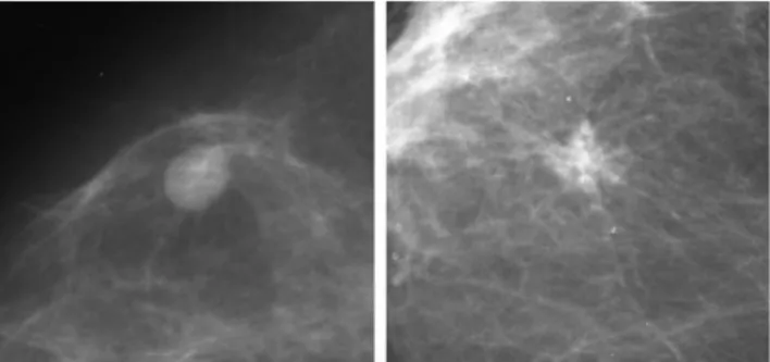
In this paper we applied CNNs to the problem of mammographic lesion classification into benign or malign. Fig. 1 shows the difference between both types of lesions mentioned before, note that regular contours are compatible with benign lesions while an irregular form are associated with malignancy [7]. Therefore, we studied the use of three different types of CNN implementations and also studied their behaviour when used with images that were, or were not, normalized in order to understand the impact of normalization on the lesion classification results.

Fig. 1. Example of benign lesion on the left and malign lesion on the right.

The paper is organized as follows: the next section presents the related work, Sections 3 and 4 present our proposal and the results obtained, respectively, the final section contains the conclusions.

2 Related Work

Deep learning-based approaches have recently shown potential for applications in digital pathology. Since 2012, these methods are used in major computer vision competitions, for example the ImageNet Large Scale Visual Recognition Competition (ILSVRC), showing the best performance in its class [11]. In [12], it is mentioned that ConvNet has proved to be the best technique for image classification and that it was used by the top 10 teams in ILSVRS-2014.

Convolutional Neural Networks have already been used by other researchers in the medi-cal image field and specifimedi-cally in the mammographic image field. Our study has been initially guided by the work of Arevalo et al. [1], who proposed a new method that was applied to the BCDR-F03 (Film Mammography Dataset Number 3) dataset from Breast Cancer Digital Repository. The method includes baseline descriptors, such as Handcraft features (HCfeats), Histogram of oriented gradients (HOG) and Histogram of gradient divergence (HGD), in a supervised feature learning approach that incorporates a CNN. For image classification, the

activations from the penultimate layer were extracted and used as input of an Support Vec-tor Machine (SVM). The authors also used different CNN models (CNN2, which consists in a single connected layer combined with a fully connected layer, CNN3, which consists in two convolutional layers and a fully connected layer and DeCAF - a pre-trained model with ImageNet) obtaining AUC values of 0.821, 0.860 and 0.836, respectively, when combined with HCfeats, and nearly 0.76, 0.82 and 0.79, respectively when used standalone. Wichakam et al.[12] published another study that combined deep convolutional networks, used as an automatic feature extraction tool, and SVM, used as classifiers, for mass detection on digi-tal mammograms and applied them to the INBreast dataset. Different approaches at the deep convolutional networks allowed reaching the best performace of 98.44% accuracy (with the SVM-FC1 of the A3 architecture).

3 Lesion Classification using CNNs with Transfer Learning

3.1 Transfer Learning for Lesion Classification

In this paper, we propose to study the application of several classification models and pre-processing strategies for mass detection in digitized mammograms.

It is well known that CNNs require large amounts of data to be properly trained. In the medical field it is usually difficult to obtain such large datasets, which is due not only to the limited number of exams produced in a single facility, but also to the amount of work that is needed for hand labeling of the samples. So, our work will be based on a transfer learning approach; we will re-use convolutional neural networks that were previously trained for a different task, and fine-tune them to our current problem.

The three different pre-trained models used in this paper were previously used to perform classification in the ImageNet ILSVRC challenge data: CNN-F (Fast, imagenet-vgg-f) and CNN-M (Medium, imagenet-vgg-m) models [2] and Caffe reference model [5]. We have then fine-tuned the networks in order to achieve the classification of benign or malign lesions from the mammographic images.

In order to apply the pre-trained models to our problem, we have adapted the software MatConvNet [10] available for Matlab. We also emphasize that we have only used CNNs as classifier, which means that, for this work, we did not use SVMs or handcrafted features.

3.2 The network

As mentioned before, three different pre-trained models were used in this work: F, CNN-M and Caffe. Table 1 presents the differences between each model. In Convolutional Layers, the ’num×size×size’ set indicates the number of convolution filters and their receptive field size. The indications ’st.’ and ’pad.’ represent the convolution stride and the spatial padding, whereas the LRN is the Local Response Normalization with or without max-pooling down-sampling factor. In the fully connected layers (’Full’), the number indicates their dimension-ality; besides, ’Full6’ and , ’Full7’ are regularized using dropout and the last layer is the soft-max classifier. Except for the last layer, the Rectification Linear Unit (RELU) is the activation function for all weight layers [2].

The architecture of the CNN-F model consist in 8 learnable layers (5 convolutional layers and 3 fully-connected layers), and the fast processing is guaranteed by the 4 pixel stride in the first convolutional layer [2].

In the first convolutional layer, the CNN-M architecture has a decreased stride and smaller receptive field and in the second convolutional layer has a larger stride keeping the computa-tion time reasonable [2].

The Caffe reference model, like the others mentioned before, has a complete set of layers that are used for visual tasks such as classification and trains models by the fast and standard stochastic gradient descent algorithm [5].

Table 1. Convolution Neural Network pretrained models (adapted from [2])

Archit. Conv1 Conv2 Conv3 Conv4 Conv5 Full6 Full7 Full8

CNN-F 64×11×11 st.4,pad.0 LRN, ×2pool 256×5×5 st.1,pad.2 LRN, ×2pool 256×3×3 st.1,pad.1 256×3×3 st.1,pad.1 256×3×3 st.1, pad.1 ×2poll 4096 drop-out 4096 drop-out 1000 soft-max CNN-M 96×7×7 st.2,pad.0 LRN, ×2pool 256×5×5 st.2,pad.1 LRN, ×2pool 512×3×3 st.1,pad.1 512×3×3 st.1,pad.1 512×3×3 st.1,pad.1 ×2poll 4096 drop-out 4096 drop-out 1000 soft-max Caffe 96×11×11 st.4,pad.0 LRN, ×2pool 256×5×5 st.1,pad.2 LRN, ×2pool 384×3×3 st.1,pad.1 384×3×3 st.1,pad.1 256×3×3 st.1,pad.1 ×2pool 4096 drop-out 4096 drop-out 1000 soft-max 3.3 Dataset

We used the BCDR-FM dataset (Film Mammography Dataset) from Breast Cancer Digi-tal Repository (http://bcdr.inegi.up.pt), which includes 1125 studies with 3703 medio-lateral oblique (MLO) and craniocaudal (CC) images of 1010 patient cases, mostly female gender (998), from 20 to 90 years old. The dataset also contains 1044 identified - and clinically de-scribed - lesions, 1517 manually-made segmentation’s and BI-RADS classification carried out by specialized radiologists [1].

The downloaded dataset, named BCDR-F03 - ”Film Mammography Dataset Number 3”, which is a subset of the BCDR-FM, comprises 736 grey-level digitized mammograms (426 benign and 310 malign mass lesions) from 344 patients. These are distributed into MLO and CC views with image size of 720×1168 (width×height) pixels and a bit depth of 8 bits per pixel in TIFF format; included are also clinical data and image-based descriptors. Although a digital dataset is available, we used the digitized dataset to enable the comparison with the work of [1]; furthermore, digital images have a bigger bit depth of 14 bits per pixel.

The pre-processing stage of our work is similar to the one used in [1], namely: cropping a ROI of 150×150 pixels using the information of the bounding box of the segmented region, the aspect ratio is always preserved, even when the lesion’s dimensions are bigger than 150×150.

However, when the lesion is next to the border of the image we translate the square crop, thus changing image coordinates and including the surrounding breast pattern, instead of zero-padding the outer portion of the crop; data augmentation using a combination of flipping and 90, 180 and 270 degrees rotation transformations.

3.4 Image Normalization

The data normalization procedure used in this work is similar to the one proposed by [1]; it consists in a Global Contrast Normalization (GCN), obtained by subtracting the mean of the intensities in the image (calculated per image and not per pixel) to each pixel, and a Local Contrast Normalization (LCN)[1]. We assessed if the use, or not, of a data normalization procedure has impact on the classification results.

3.5 Experiments

Following the authors’ indications in [1], we divided images into three groups: 50% for train-ing, 10% for validation and 40% for testing. The images’ input size for the different models was 224×224 pixels; the parameters’ exploration space comprised three fully connected lay-ers, 50 epochs, fc8 is a initially-randomized layer, five learning rate values (1e-2, 1e-3, 1e-4, 5e-2, 5e-3 and 5e-4), the three pre-trained models (vgg-f, vgg-m and caffe) and the use, or not, of normalized images; see Fig. 2.

After the fine tuning of the three networks using the train and the validation sets (which comprise 2800 and 560 images, respectively) with and without normalization, we chose the best parameters to apply to the test set (comprised of 2240 images); this time, the training set comprised 3360 images due to the merge of the initial training and validation.

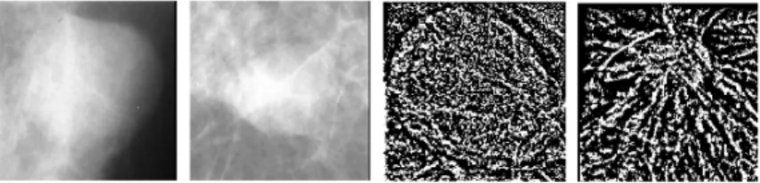
Fig. 2. Examples of 150×150 crop images. On the left two images without normalization and on the right images with normalization.

4 Results and Discussion

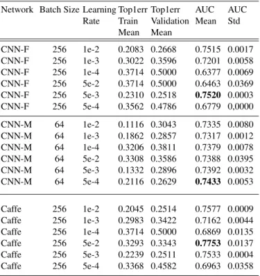
The results of the parameters’ exploration are shown in Tables 2 and 3. With normalized training and validation sets, the best mean AUC was achieved by the Caffe reference model (AUC mean = 0.7753, std = 0.0135), followed by the CNN-F model (AUC mean = 0.7520 std = 0.0003) and the CNN-M (AUC mean = 0.7392, std = 0.0032).

Relatively to the training and validation sets without normalization, the best AUC mean was achieved by the CNN-M model (AUC mean = 0.7846, std = 0.0034), followed by the

Table 2. CNN parameter exploration, with five repetitions, using normalized images (only the train and validation sets were used).

Network Batch Size Learning Rate Top1err Train Mean Top1err Validation Mean AUC Mean AUC Std CNN-F 256 1e-2 0.2083 0.2668 0.7515 0.0017 CNN-F 256 1e-3 0.3022 0.3596 0.7201 0.0058 CNN-F 256 1e-4 0.3714 0.5000 0.6377 0.0069 CNN-F 256 5e-2 0.3714 0.5000 0.6463 0.0369 CNN-F 256 5e-3 0.2310 0.2518 0.7520 0.0003 CNN-F 256 5e-4 0.3562 0.4786 0.6779 0,0000 CNN-M 64 1e-2 0.1116 0.3043 0.7335 0.0080 CNN-M 64 1e-3 0.1862 0.2857 0.7317 0.0012 CNN-M 64 1e-4 0.3206 0.3811 0.7379 0.0078 CNN-M 64 5e-2 0.3308 0.3586 0.7388 0.0395 CNN-M 64 5e-3 0.1332 0.2896 0.7392 0.0032 CNN-M 64 5e-4 0.2116 0.2629 0.7433 0.0053 Caffe 256 1e-2 0.2045 0.2514 0.7577 0.0009 Caffe 256 1e-3 0.2983 0.3422 0.7162 0.0044 Caffe 256 1e-4 0.3714 0.5000 0.6869 0.0135 Caffe 256 5e-2 0.3293 0.3343 0.7753 0.0137 Caffe 256 5e-3 0.2239 0.2511 0.7533 0.0004 Caffe 256 5e-4 0.3368 0.4582 0.6963 0.0358

Caffe reference model (AUC mean = 0.7688, std = 0.0019) and the CNN-F model (AUC mean = 0.7626, std = 0.0044).

Once the best combination of parameters to each model was determined, new results were obtained using the testing set (and the new merged training set); these are presented in Table 4. It is possible to see that we achieved the best AUC mean of 0.8126 (std=0.001) with Caffe reference model with no normalized images, surpassing the result in [1] of 0.79 obtained with DeCAF (an old version of Caffe) with normalized images (and with a SVM instead of a softmax layer, since they consider that the former has better performance as classifier than the latter.

As it happened with validation set, the best AUC results were achieved using images with-out normalization, namely 0.7764 with CNN-M and 0.7671 with CNN-F, which are similar values to the ones obtained during the fine-tuning stage. The AUC results with normalized images are lower than those obtained with the validation set, especially the results of Caffe that was substantially lower, AUC=0.5842 (previous one was 0.7753).

Table 3. CNN parameter exploration, with five repetitions, using images with no normalization (only the train and validation sets were used).

Network Batch Size Learning Rate Top1err Train Mean Top1err Validation Mean AUC Mean AUC Std CNN-F 256 1e-2 0.2028 0.3261 0.7626 0.0044 CNN-F 256 1e-3 0.2544 0.3614 0.7477 0,0179 CNN-F 256 1e-4 0.3714 0.5000 0.6857 0.0133 CNN-F 256 5e-2 0.3701 0.4825 0.7447 0.0047 CNN-F 256 5e-3 0.2060 0.3096 0.7618 0.0060 CNN-F 256 5e-4 0.3360 0.4204 0.6958 0.0125 CNN-M 64 1e-2 0.0945 0.2654 0.7565 0.0189 CNN-M 64 1e-3 0.1501 0.2653 0.7809 0.0049 CNN-M 64 1e-4 0.2322 0.3529 0.7647 0.0030 CNN-M 64 5e-2 0.2029 0.3336 0.7420 0.0399 CNN-M 64 5e-3 0.1065 0.2700 0.7597 0.0091 CNN-M 64 5e-4 0.1695 0.2697 0.7846 0.0034 Caffe 256 1e-2 0.1766 0.3225 0.7674 0.0034 Caffe 256 1e-3 0.2295 0.3757 0.7645 0.0041 Caffe 256 1e-4 0.3714 0.5000 0.6796 0,0209 Caffe 256 5e-2 0.3449 0.4246 0.7397 0.0133 Caffe 256 5e-3 0.1903 0.3246 0.7688 0.0019 Caffe 256 5e-4 0.2810 0.3811 0.7563 0.0031

Table 4. CNN applied to images with and without normalization. Training on the training plus validation sets and testing on the test set.

Network Batch Size Epochs Learning Rate Norm Top1err Train Mean Top1err Test Mean AUC Mean AUC Std CNN-F 256 50 5e-3 Yes 0.1964 0.3782 0.7206 0.0008 CNN-F 256 50 1e-2 No 0.1714 0.2955 0.7671 0.0022 CNN-M 64 50 5e-4 Yes 0.1727 0.3554 0.7332 0.0021 CNN-M 64 50 5e-4 No 0.1460 0.2876 0.7764 0.0059 Caffe 256 50 5e-2 Yes 0.3235 0.4883 0.5842 0.0038 Caffe 256 50 5e-3 No 0.1902 0.2507 0.8126 0.0010

5 Conclusions

In this paper we studied the application of CNNs to the problem of mammogram lesion classi-fication. We evaluated three different implementations of CNNs and two approaches of image normalization.

In terms of the results obtained with the three different CNNs implementations, in the case of the normalized images with the validation set, the best result was obtained with the Caffe model, followed by the CNN-F and then the CNN-M. This is somewhat surprising given that the CNN-M is a more powerful model (the filters are larger) than the CNN-F. The difference is not large though (0.0087). However, when we applied the networks to the testing set, the results decreased substantially, mostly in Caffe model with a AUC of 0.5842.

When the images where fed to the networks without normalization, with the validation set the results were better for the Caffe and CNN-M but were worse for the CNN-F (again a small difference). The CNN-M did improve by a significant amount (from an AUC of 0.7433 to 0.7846). In the testing set, the Caffe model achieved the best AUC (0.8126), followed by CNN-M and CNN-F, 0.7764 and 0.7671, respectively.

Regarding the image normalization, the results reveal that the normalization process pro-posed in [1] decreases the performance of networks’ classification. The fact that all images were composed by the surrounding breast pattern (instead of being painted black, for exam-ple) and, in some cases that the lesion was not centered, may have been an advantage for the CNN learning process without confounding factors.

As future work we intend to explore other normalization approaches, the combination of CNNs with SVMs and also the inclusion of handcraft features to see if they can help increase the classification accuracy.

6 Acknowledgments

This work was supported by National Funding from the FCT - Fundac¸˜ao para a Ciˆencia e a Tecnologia, through the UID/EEA/50008/2013 Project. The GTX Titan X used in this research was donated by the NVIDIA Corporation.

The database used in this work was a courtesy of MA Guevara and coauthors, Breast Cancer Digital Repository Consortium.

References

1. Arevalo, J., Gonz´alez, F.A., Ramos-Poll´an, R., Oliveira, J.L., Guevara Lopez, M.A.: Rep-resentation learning for mammography mass lesion classification with convolutional neu-ral networks. Computer Methods and Programs in Biomedicine 127, 248–257 (2016) 2. Chatfield, K., Simonyan, K., Vedaldi, A., Zisserman , A.: Best Scientific Paper Award

Return of the Devil in the Details: Delving Deep into Convolutional Nets British Machine Vision Conference, 2014. Available via arxiv.org.

https://arxiv.org/pdf/1405.3531v4.pdf

3. Ganesan, K., Acharya, U.R., Chua, C.K., Min, L.C., Abraham, K.T., Ng, K.H.: Computer-aided breast cancer detection using mammograms: a review. IEEE Reviews in Biomedical Engineering. 6, 77–97 (2013)

4. Jalalian, A., Mashohor, S., Mahmud, H., Saripan, M., Ramli, A., Karasfi, B.: Computer-aided detection/diagnosis of breast cancer in mammography and ultrasound: a review. Clinical Imaging 37, 420–426 (2013)

5. Jia, Yangqing and Shelhamer, Evan and Donahue, Jeff and Karayev, Sergey and Long, Jonathan and Girshick, Ross and Guadarrama, Sergio and Darrell, Trevor: Caffe: Con-volutional Architecture for Fast Feature Embedding. arXiv preprint arXiv:1408.5093. (2014)

6. Jiao, Z., Gao, X., Wang, Y., Li, J.: A deep feature based framework for breast masses classification. Neurocomputing.197, 221–231 (2016)

7. Pisco, Joo Martins: Imagiologia Bsica Texto e Atlas 1st Edition. LIDEL, Lisboa (2003) 8. Sampat, M., Markey, M., Bovik, A.: Computer-Aided Detection and Diagnosis in

Mam-mography. Handbook of Image and Video Processing. , 1195–1217 (2005)

9. Tang, J.S., Agaian, S., Thompson, I.: Guest Editorial: Computer-Aided Detection or Di-agnosis (CAD) Systems. IEEE Systems Journal.8, 907–909 (2014)

10. Vedaldi, A., Lenc, K.: MatConvNet – Convolutional Neural Networks for MATLAB. Proceeding of the ACM Int. Conf. on Multimedia (2015).

11. Wang, D., Khosla, A., Gargeya, R., Irshad, H., Beck, A.H..: Deep Learning for Iden-tifying Metastatic Breast Cancer. In: Cornell University Library (2016) Available via arxiv.org.

https://arxiv.org/pdf/1606.05718.pdf. Cited 14 March 2017

12. Wichakam, I., Vateekul, P.: Combining deep convolutional networks and SVMs for mass detection on digital mammograms. 2016 8th International Conference on Knowledge and Smart Technology (KST)., 239–244 (2016)