Joana Ferreira Guerreiro
Licenciada em Ciências e Engenharia do Ambiente
Assessment of NDVI, Land Surface Temperature and
Precipitation anomalies for drought monitoring in
Bayankhongor province, Mongolia.
Dissertação submetida para obter o Grau de Mestre em Engenharia do
Ambiente, Perfil de Engenharia de Sistemas Ambientais
Orientadora: Prof. Doutora Maria Júlia Seixas, Professora Auxiliar, FCT/UNL
Co-orientador: Doutor Nuno Santos Grosso, DEIMOS Engenharia SA
Júri:
Presidente da mesa: Prof.ª Doutora Maria Teresa Calvão Rodrigues
Vogais: Doutor Nuno Miguel Matias Carvalhais Prof.ª Doutora Maria Júlia Fonseca de Seixas
Assessment of NDVI, Land Surface Temperature and Precipitation anomalies for drought
monitoring in Bayankhongor province, Mongolia.
Copyright © Joana Ferreira Guerreiro, FCT/UNL, UNL.
A Faculdade de Ciências e Tecnologia e a Universidade Nova de Lisboa têm o direito, perpétuo
e sem limites geográficos, de arquivar e publicar esta dissertação através de exemplares
impressos reproduzidos em papel ou de forma digital, ou por qualquer outro meio conhecido ou
que venha a ser inventado, e de a divulgar através de repositórios científicos e de admitir a sua
cópia e distribuição com objetivos educacionais ou de investigação, não comerciais, desde que
Acknowledgments
This thesis represents a milestone in six years of studying in FCT-UNL and I wouldn’t been able
to finish it without the guidance and support of several individuals.
First, I would like to thank my academic advisor, Professor Maria Júlia Seixas, for awakening my
interest in remote sensing and being always available to answers my questions. Her mentoring,
useful remarks and sympathy over the course of this experience helped me in all the time of
writing this thesis.
I would also like to thank my co-advisor, Dr. Nuno Grosso, for the opportunity to work with a
company outside the faculty which contributed to make my thesis experience richer and
productive. All the encouragement through the learning process of this thesis was motivating and
his patience and friendly personality through the hours devoted to finding and understanding
errors in my python programs were greatly appreciated.
I acknowledge my gratitude to everyone in DEIMOS Engenharia, for receiving me with arms wide
open which made my experience much more stimulating. A special thanks to Carla Patinha, for
always being available to send me the necessary information with a smile on her face.
I take this opportunity to show my gratitude to my parents for their love and continuous support
throughout my life. They always encouraged me and gave me the strength to reach my goals and
chase my dreams. Thank you for your patience and comprehension during the long days in front
of the computer when no one could speak or make any noise. You are my safe haven!
To my boyfriend, Fábio Santos, I wish to offer my deepest thanks. He stood by me cheering me
up through the process, even when I retreated to long days in the company of my computer. You
are my rock and your support and faith in me makes me a better person. You make my life fuller
and I want to thank you for always being there when I need you the most.
I would like to thank my best friends, Rita and Katy, for giving a meaning to the expression “true
friendship”. Rita we’ve been through so much together in these 23 years. Despite going our
separate ways we’ve always managed to be true to ourselves and stay close to one another.
Thank you for always showing up in the most important days. Katy, you’ve become my partner in
crime and my confidant. We are so different, yet so close and that’s what makes our friendship
so unique. Thank you for being there for me all these years smiling, studying, crying, laughing,
talking, singing… being my friend.
Andreia and Afonso, I want to thank you for your friendship and support. My life has become
happier and funnier since that first math class. Sandra and Carol, thank you for being the proof
that high school friends can stay in our lives and support each other through the years.
Finally, I would like to thank my family and all the friends who supported me and made the writing
Abstract
During the last decade Mongolia’s region was characterized by a rapid increase of both severity and frequency of drought events, leading to pasture reduction. Drought monitoring and assessment plays an important role in the region’s early warning systems as a way to mitigate the negative impacts in social, economic and environmental sectors. Nowadays it is possible to
access information related to the hydrologic cycle through remote sensing, which provides a
continuous monitoring of variables over very large areas where the weather stations are sparse.
The present thesis aimed to explore the possibility of using NDVI as a potential drought indicator
by studying anomaly patterns and correlations with other two climate variables, LST and
precipitation. The study covered the growing season (March to September) of a fifteen year
period, between 2000 and 2014, for Bayankhongor province in southwest Mongolia. The datasets
used were MODIS NDVI, LST and TRMM Precipitation, which processing and analysis was
supported by QGIS software and Python programming language. Monthly anomaly correlations
between NDVI-LST and NDVI-Precipitation were generated as well as temporal correlations for
the growing season for known drought years (2001, 2002 and 2009).
The results show that the three variables follow a seasonal pattern expected for a northern
hemisphere region, with occurrence of the rainy season in the summer months. The values of
both NDVI and precipitation are remarkably low while LST values are high, which is explained by the region’s climate and ecosystems. The NDVI average, generally, reached higher values with high precipitation values and low LST values. The year of 2001 was the driest year of the
time-series, while 2003 was the wet year with healthier vegetation.
Monthly correlations registered weak results with low significance, with exception of NDVI-LST
and NDVI-Precipitation correlations for June, July and August of 2002. The temporal correlations
for the growing season also revealed weak results. The overall relationship between the variables
anomalies showed weak correlation results with low significance, which suggests that an accurate
answer for predicting drought using the relation between NDVI, LST and Precipitation cannot be
given. Additional research should take place in order to achieve more conclusive results. However
the NDVI anomaly images show that NDVI is a suitable drought index for Bayankhongor province.
Resumo
Na última década, a região da Mongólia foi caracterizada por um rápido aumento da frequência
e severidade de eventos de seca, levando à redução de pastagens. A avaliação e monitorização
da seca tem um papel importante nos sistemas de alerta da região como uma forma de mitigar
os impactes negativos nos sectores social, económico e ambiental. Indicadores e índices de seca
são utilizados para caracterizar a severidade, dimensão espacial e duração das secas.
Atualmente é possível aceder a informação relacionada com o ciclo hidrológico através da
deteção remota, o que permite uma monitorização contínua de variáveis ao longo de áreas
maiores onde estações meteorológicas não tem uma expressão tão significativa.
A presente tese teve como objetivo, explorar a possibilidade de utilizar o NDVI como potencial
indicador de seca, através do estudo de padrões de anomalias e correlações com outras duas
variáveis climáticas (LST e precipitação). O estudo teve como dimensão temporal o período de
crescimento vegetativo (Março a Setembro) de um intervalo de tempo de quinze anos
(2000-2014) para a província de Bayankhongor no sudueste da Mongólia. Os data sets utilizados foram
NDVI e LST do MODIS e a Precipitação da TRMM, cujo processamento e análise foi suportado
pelo software QGIS e a linguagem de programação Python. Foram calculadas correlações
mensais de anomalias entre NDVI-LST e NDVI-precipitação, assim como correlações temporais
para o período de crescimento vegetativo para três anos de seca conhecidos (2001,2002 e 2009).
Os resultados mostraram que as três variáveis seguem um padrão sazonal expectável para uma
região do hemisfério norte, cujo período de chuvas ocorre nos meses de Verão. Os valores de
NDVI e precipitação são notavelmente baixos enquanto os valores de LST são elevados, o que
é explicado pelo clima e ecossistemas da região. O ano de 2001 foi o mais seco da série temporal
e 2003 foi o ano com maior crescimento vegetativo. No geral, a média de NDVI atingiu valores
mais elevados quando os valores de precipitação eram também mais elevador e os valores de
LST mais baixos, o que evidencia uma possível correlação positiva com a precipitação e uma
correlação negativa com a LST.
As correlações mensais registaram resultados fracos e com pouca significância, à exceção das
correlações entre NDVI-LST e NDVI-precipitação para Junho, Julho e Agosto de 2002. As
correlações temporais para o período de crescimento vegetativo e para a combinação de Junho,
Julho e Agosto, também revelaram resultados fracos. No geral, as relações entre as anomalias
das três variáveis em estudo apresentaram baixas correlações com resultados pouco
significativos, o que sugere que a previsão de secas baseada na relação entre NDVI, LST e a
Precipitação ainda está por determinar. Estudos adicionais deverão ser levados a cabo de forma
a obter resultados mais fiáveis e conclusivos. Contudo, as imagens obtidas para as anomalias
de NDVI sugerem que este é um bom indicador de seca para a província de Bayankhongor.
Palavras-chave: Anomalia, Correlação, Deteção Remota, Indicador de Seca, LST, NDVI,
Table of Contents
Acknowledgments ... iii
Abstract ... v
Resumo ... vii
Table of Contents ... ix
List of Figures ... xi
List of Tables ... xv
Acronyms ... xvii
1. Introduction... 19
1.1. Motivation, Scope and Objectives ... 20
1.2. Thesis outline ... 20
2. Literature Review ... 23
2.1. Drought concepts ... 23
2.2. Drought in the Mongolia’s region ... 24
1.1. Drought Monitoring through Earth Observation data ... 25
2.3. NDVI as a drought indicator ... 27
3. Materials and Methods ... 31
3.1. Study Area ... 31
3.2. Datasets Description ... 32
3.2.1. NDVI ... 32
1.1.1. Land Surface Temperature ... 32
3.2.2. Precipitation ... 32
3.3. Methodology ... 33
3.3.1. Data pre-processing ... 33
3.3.1.3. Precipita ... 37
3.3.2. Data Analysis ... 37
4. Results and Discussion ... 39
4.1. Exploratory Analysis ... 39
4.1.1. NDVI ... 39
4.1.2. Land Surface Temperature ... 44
4.1.3. Precipitation ... 49
4.2. Monthly correlations of data sets anomalies for drought years ... 54
4.3. Spatial Distribution of NDVI correlations ... 55
4.3.1. NDVI-LST ... 55
4.3.2. NDVI-Precipitation ... 58
5. Conclusions ... 63
6. References ... 65
7. Appendixes ... 69
Appendix A – Python programs ... 69
Appendix A.1 Convert HDF to TIF (LST) ... 69
Appendix A.2 Convert NC to TIF, Clip and Calculate Mean (Precipitation) ... 71
Appendix A.3 Clip Bayankhongor province from raster ... 75
Appendix A.4 Multiply by scale factor and apply QC mask ... 77
Appendix A.5 Monthly average ... 79
Appendix A.6 Anomaly calculation ... 81
Appendix A.7 Resample to coarser resolution ... 85
Appendix A.8 Pearson Correlation ... 87
Appendix A.9 Pixelwise correlation between datasets ... 89
Appendix A.10 Save data to csv file ... 93
Appendix B Montlhy NDVI anomalies ... 95
Appendix C – Spatial Distribution of Monthly NDVI anomalies ... 97
Appendix D – Monthly Land Surface Temperature anomalies ... 111
Appendix E – Spatial Distribution of Land Surface Temperature anomalies ... 113
Appendix F – Monthly Precipitation anomalies ... 125
Appendix G – Spatial Distribution of Precipitation anomalies ... 127
List of Figures
Figure 2.1 | Current and future satellite missions relevant to drought monitoring and assessment ... 26
Figure 3.1 | Bayankhongor province location (red outline) and Mongolia’s natural zones. (Adapted from Finch, C.(ed). Mongolia’s wild heritage: Biological Diversity, Protected Areas, and Conservation in the Land of Chingis Khan. Boulder, CO: Avery Press, 1999.) ... 31
Figure 3.2 | Growing season datasets timeline with LST and NDVI following the Julian calendar. ... 33
Figure 3.3 | Schematic representation of the methodology used ... 34
Figure 3.4 | Schematic representation of NDVI data pre-processing for each month. ... 35
Figure 3.5 | Sinusoidal world tile grid with Bayankhongor tiles in yellow. (National Aeronautics and Space Administration, Goddard Space Flight Center, 2013) ... 36
Figure 3.6 | Schematic representation of the concept behind the temporal correlation between two datasets. ... 38
Figure 4.1 | Normalized Difference Vegetation Index monthly averages for the time period 2000-2014. ... 40
Figure 4.2 | NDVI Anomalies for March, May, July and September, with reference to the respective monthly average for the period 2000-2014. ... 41
Figure 4.3 | Spatial distribution of NDVI anomalies for a standard, dry and wet year (March and May) ... 42
Figure 4.4 | Spatial distribution of NDVI anomalies for a standard, dry and wet year (July and September) ... 43
Figure 4.5 | Land Surface Temperature monthly averages for the time period 2000 – 2014. ... 45
Figure 4.6 | LST Anomalies (°C) for March, May, July and September, with reference to the respective monthly average for the period 2000-2014. ... 46
Figure 4.7 | Spatial distribution of LST anomalies (°C) for a standard, dry and wet year, for the months of March and May. ... 47
Figure 4.8 | Spatial distribution of LST anomalies (°C) for a standard, dry and wet year, for the months of July and September. ... 48
Figure 4.9 | Precipitation monthly averages for the time period 2000 – 2014. ... 50
Figure 4.10 | Precipitation Anomalies (mm) for March, May, July and September, with reference to the respective monthly average for the period 2000-2014. ... 51
Figure 4.11 | Spatial distribution of precipitation anomalies (mm) for a standard, dry and wet year, for the months of March and May. ... 52
Figure 4.12 | Spatial distribution of precipitation anomalies (mm) for a standard, dry and wet year, for the months of July and September. ... 53
Figure 4.13 | Spatial distribution of temporal correlations between NDVI and LST anomalies for the growing season of 2001. Significant values for p < 0,1. ... 56
Figure 4.14 | Spatial distribution of temporal correlations between NDVI and LST anomalies for the growing season of 2002. Significant values for p < 0,1. ... 57
Figure 4.15 | Spatial distribution of temporal correlations between NDVI and LST anomalies for the growing season of 2009. Significant values for p < 0,1. ... 57
Figure 4.16 | Spatial distribution of temporal correlations between NDVI and Precipitation anomalies for the growing season of 2001. Significant values for p < 0,1. ... 60
Figure 4.18 | Spatial distribution of temporal correlations between NDVI and Precipitation anomalies for the
growing season of 2009. Significant values for p < 0,1. ... 61
Figure 7.1 | NDVI Anomalies for March, April, May and June, with reference to the respective monthly average for the period 2000-2014. ... 95
Figure 7.2 | NDVI Anomalies for July, August and September, with reference to the respective monthly average for the period 2000-2014. ... 96
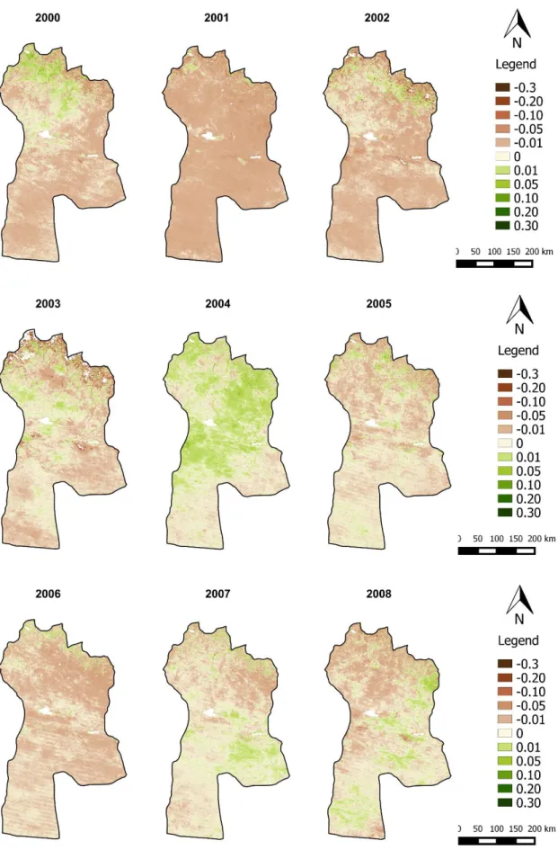
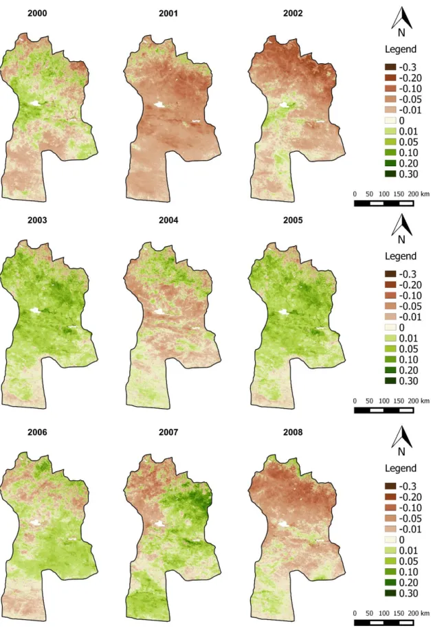
Figure 7.3 | Spatial distribution of NDVI anomalies of March for the period 2000 – 2008. ... 97
Figure 7.4 | Spatial distribution of NDVI anomalies of March for the period 2009 – 2014. ... 98
Figure 7.5 | Spatial distribution of NDVI anomalies of April for the period 2000 – 2008. ... 99
Figure 7.6 | Spatial distribution of NDVI anomalies of April for the period 2009 – 2014. ... 100
Figure 7.7 | Spatial distribution of NDVI anomalies of May for the period 2000 – 2008. ... 101
Figure 7.8 | Spatial distribution of NDVI anomalies of May for the period 2009 – 2014. ... 102
Figura 7.9 | Spatial distribution of NDVI anomalies of June for the period 2000 – 2008. ... 103
Figura 7.10 | Spatial distribution of NDVI anomalies of June for the period 2009 – 2014. ... 104
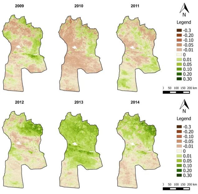
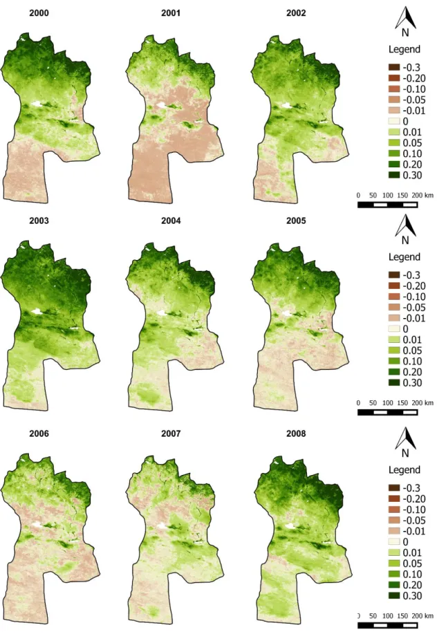
Figure 7.11 | Spatial distribution of NDVI anomalies of July for the period 2000 – 2008. ... 105
Figure 7.12 | Spatial distribution of NDVI anomalies of July for the period 2009 – 2014. ... 106
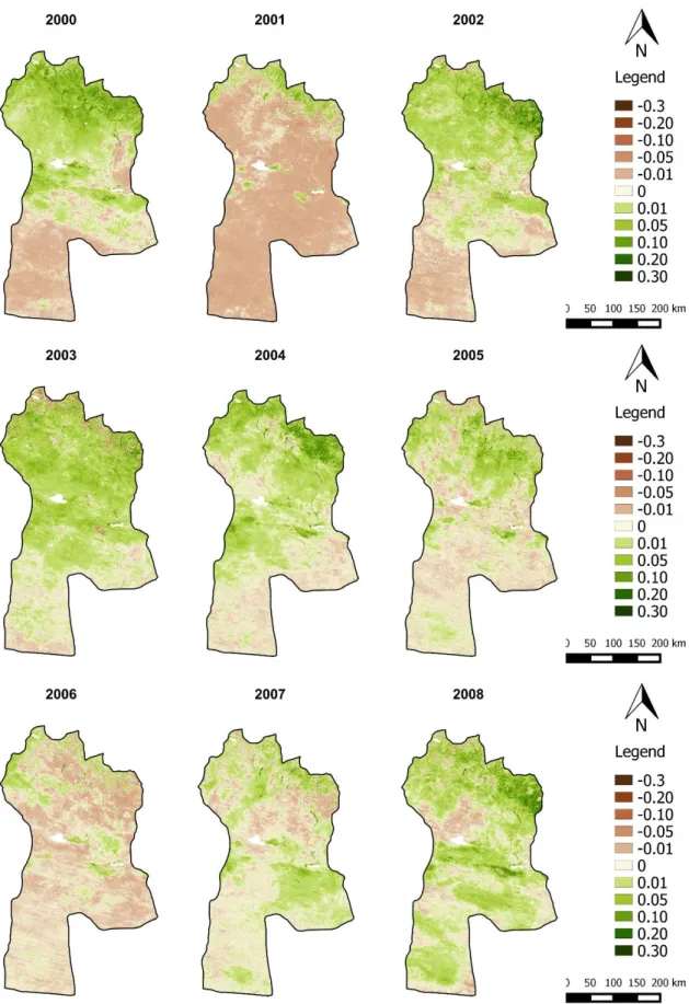
Figura 7.13 | Spatial distribution of NDVI anomalies of August for the period 2000 – 2008. ... 107
Figura 7.14 | Spatial distribution of NDVI anomalies of August for the period 2009 – 2014. ... 108
Figura 7.15 | Spatial distribution of NDVI anomalies of September for the period 2000 – 2008... 109
Figura 7.16 | Spatial distribution of NDVI anomalies of September for the period 2009 – 2014... 110
Figure 7.17 | Land Surface Temperature anomalies for the time series 2000-2014 (March – June) (ºC) . 111 Figure C7.18 | Land Surface Temperature anomalies for the time series 2000-2014 (July – September) (ºC) ... 112
Figure 7.19 | Spatial distribution of LST anomalies of March for the period 2000 – 2008. ... 113
Figura 7.20 | Spatial distribution of LST anomalies of March for the period 2009 – 2014. ... 114
Figura 7.21 | Spatial distribution of LST anomalies of April for the period 2000 – 2008. ... 115
Figura 7.22 | Spatial distribution of LST anomalies of April for the period 2009 – 2014. ... 116
Figura 7.23 | Spatial distribution of LST anomalies of May for the period 2000 – 2008. ... 117
Figura 7.24 | Spatial distribution of LST anomalies of May for the period 2009 – 2014. ... 118
Figura 7.25 | Spatial distribution of LST anomalies of June for the period 2000 – 2008. ... 119
Figura 7.26 | Spatial distribution of LST anomalies of June for the period 2009 – 2014. ... 120
Figura 7.27 | Spatial distribution of LST anomalies of July for the period 2000 – 2008. ... 121
Figura 7.28 | Spatial distribution of LST anomalies of July for the period 2009 – 2014. ... 122
Figura 7.29 | Spatial distribution of LST anomalies of September for the period 2000 – 2008. ... 123
Figura 7.30 | Spatial distribution of LST anomalies of September for the period 2009 – 2014. ... 124
Figure D7.31 | Precipitation for the time series 2000-2014 (March – June) (mm/h) ... 125
Figure D7.32 | Precipitation for the time series 2000-2014 (July – September) (mm/h) ... 126
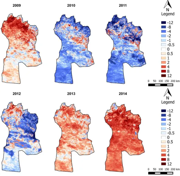
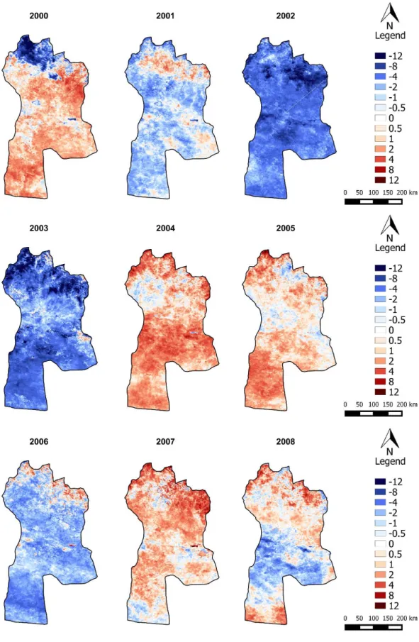
Figure 7.33 | Spatial distribution of precipitation anomalies of March for the period 2000 – 2008. ... 127
Figure 7.34 | Spatial distribution of precipitation anomalies of March for the period 2009 – 2014. ... 128
Figure 7.35 | Spatial distribution of precipitation anomalies of April for the period 2000 – 2008. ... 129
Figure 7.36 | Spatial distribution of precipitation anomalies of April for the period 2009 – 2014. ... 130
Figure 7.37 | Spatial distribution of precipitation anomalies of May for the period 2000 – 2008. ... 131
Figure 7.38 | Spatial distribution of precipitation anomalies of May for the period 2009 – 2014. ... 132
Figure 7.41 | Spatial distribution of precipitation anomalies of July for the period 2000 – 2008. ... 135
Figure 7.42 | Spatial distribution of precipitation anomalies of July for the period 2009 – 2014. ... 136
Figure 7.43 | Spatial distribution of precipitation anomalies of August for the period 2000 – 2008. ... 137
Figure 7.44 | Spatial distribution of precipitation anomalies of August for the period 2009 – 2014. ... 138
Figure 7.45 | Spatial distribution of precipitation anomalies of September for the period 2000 – 2008. .... 139
Figure 7.46 | Spatial distribution of precipitation anomalies of September for the period 2009 – 2014. .... 140
List of Tables
Table 3-1 | Summary of the data sets. ... 33
Table 4-1 | Monthly correlation of NDVI, LST and Precipitation anomalies (2001). The significant
values are in bold while the highest significant correlations are in red. ... 54
Table 4-2 | Monthly correlation of NDVI, LST and Precipitation anomalies (2002). The significant
values are in bold while the highest significant correlations are in red. ... 55
Table 4-3 | Monthly correlation of NDVI, LST and Precipitation anomalies (2009). The significant
Acronyms
AVHRR - Advanced Very High Resolution Radiometer
EO – Earth Observation
EPSG - European Petroleum Survey Group
ET – Evapotranspiration
GEO – Geostationary
GIS – Geographic Information System
LEO - Low Earth Orbit
LST – Land Surface Temperature
MODIS - Moderate Resolution Imaging Spectroradiometer
NDVI – Normalized Difference Vegetation Index
QC - Quality Control
SDS – Scientific Data Sets
TRMM - Tropical Rainfall Measuring Mission
UTM - Universal Transverse Mercator
VCI – Vegetation Condition Index
WGS - World Geodesic System
1.
Introduction
Extreme climatic events have been increasing in frequency and severity worldwide over the past
century (John, et al., 2013). Drought is possibly the most complex and harmful natural hazard
since it shows a highly variability over time and space and usually extends to large geographic
areas (Senay, et al., 2015). Over the past five decades the global land area affected by drought
has increased, particularly in central and northern Eurasia (Zhang, et al., 2012).
This kind of extreme event carries a handful of impacts that span various sectors of the society
causing dire environmental, social and economic consequences. Drought is the number one
natural hazard when speaking about the number of people affected (Mishra & Singh, 2010).
Therefore, assessment and monitoring of droughts is crucial to early warning systems and management in order to mitigate drought’s serious effects.
Efforts have been made to develop and implement various quantitative measures of drought’s
extent and severity. However, it is difficult to predict and monitor using traditional approaches,
especially over large areas. The use of satellite remote sensing in drought monitoring has gained
more attention since it can be used to measure meteorological or biophysical characteristics of Earth’s surfaces (Rhee, Im, & Carbone, 2010). Technological advances in this field have enabled continuous data measurements over a range of spatial and temporal scales which can help
generate long term information on drought events (Senay, et al., 2015).
Remote sensing-based vegetation indices have been widely used for drought monitoring and
tracking. Among the vegetation indices, the Normalized Difference Vegetation Index (NDVI) is the
most common. The vegetation condition index (VCI) also measures the time of drought’s onset
and its intensity, duration and impact on vegetation. However, it is best used during growing
season when vegetation is most photosynthetically active (Mishra & Singh, 2010). Also, the
combination of vegetation indices with drought indices and data such as land surface temperature
and rainfall can be a very powerful instrument as it provides useful and more detailed information
on drought monitoring ( (Karnieli, et al., 2010), (Nichol & Abbas, 2015)).
Mongolia, already characterized by severe weather conditions due to its inland location, is one of
the regions dealing with extreme climatic events caused by climate change impacts. These events
include droughts, dzuds (harsh winters), dust storms and desertification. During the last decade
the severity and frequency of drought during the growing season has increased as well as
extreme winters, leading to pasture reduction in Mongolia which is a key economic drive of the
country (Nandintsetseg & Shinoda, 2012). The most recent extreme events in Mongolia were the
combined summer drought–dzud events of 2000–2002 and the drought-dzud event of 2009- 2010
(John, et al., 2013). Accordingly, an early warning system and a better understanding of summer
drought events is a main concern for this country in order to mitigate drought’s impacts on the
1.1. Motivation, Scope and Objectives
The motivation for this dissertation arose from the opportunity of working in satellite remote
sensing with DEIMOS Engenharia, who is developing a project for the Asian Development Bank. This project, “Climate-Resilient Rural Livelihoods in Mongolia”, aims to complement “government efforts to develop a sustainable, climate proof livestock sector, the main economic activity in
Mongolia, able to overcome the productivity and in-come loss problems, related to over-grazing and climate change, registered in recent years”. The project delivers two main services: (1) Land use/land cover mapping and Digital Elevation Model; (2) Drought monitoring, focused to enhance
the current National Remote Sensing Centre drought monitoring system which is based on
Moderate Resolution Imaging Spectroradiometer (MODIS) data. The drought monitoring service
is based on NDVI data applied to Bayankhongor province in Mongolia (DEIMOS Engenharia,
2015).
The second service being rendered by DEIMOS was the main drive for defining the purpose and
scope of the thesis. Thus, the aim of the study is to explore the possibility of using NDVI anomalies
as a drought index, based on its relation with land surface temperature (LST) and precipitation
data. The study site refers to Bayankhongor province, in southwest Mongolia, and is based in the
growing season (March to September) of a fifteen year time series (2000-2014), with a focus on
known drought years (2001, 2002 and 2009). The analysis was supported by QGIS software and
Python programming language. Several objectives were defined to lead to the main goal of the
study:
i) Calculation of NDVI, LST and Precipitation monthly anomalies for the time period
2000-2014;
ii) Assessment of correlation between NDVI, LST and Precipitation anomalies for the
drought years 2001, 2002 and 2009:
o Calculation of monthly correlations;
o Calculation of growing season temporal correlations.
iii) Exploratory analysis and interpretation of the correlation patterns between NDVI and LST
and Precipitation, by using land use and land cover maps.
1.2. Thesis outline
This document consists in five chapters, including the Introduction (this chapter), with specific
focus and objectives:
Chapter 2 - Literature Review: It describes and analyses previous research related to the
topic as well as defines important concepts. This chapter covers three main areas related to the
problem, (1) drought concepts and drought monitoring challenges, (2) using NDVI as a drought
Chapter 3 - Materials and Methods: This chapter describes the data being used and outlines
the procedures used to conduct the study. It includes four main components, (1) description of
Bayankhongor province characteristics, (2) description of the three datasets used for the study
(NDVI, LST and Precipitation), (3) data pre-processing methods as a first approach to the
datasets, and (4) data processing which describes the methodology used to generate results,
specifically anomalies calculations, monthly anomaly correlations between datasets and final time
series spatial correlation.
Chapter 4 - Results and Discussion: This chapter reports and addresses the results
generated from the previous chapter and discusses the significant findings and its meaning for
the study.
Chapter 5 - Conclusions: Identifies the critical conclusions gathered from the results and
findings discussion and relates them with the research objectives defined in the Introduction. It
includes a Limitations section, where are presented limitations encountered during the research
process, and a Further Investigation section, where it’s mentioned future research and follow-up
2.
Literature Review
2.1. Drought concepts
Drought is a complex natural hazard that carries negative impacts for people and for the
environment. It is typically characterized by type, frequency, duration, magnitude, severity and
geographic extent. However, determining a universal definition is extremely difficult due to drought’s temporal and spatial variation. A general definition of drought defines it as “an extended period – a season, a year, or several years – of deficient rainfall relative to the statistical
multi-year average for a region” (Graham, 2000)
There are four main types of droughts defined in the literature (Senay, et al., 2015):
I. Meteorological drought, which is defined by a lower precipitation than the long-term
average precipitation, for a prolonged period of time (i.e. it is based on the degree of
dryness and the duration of that dry period);
II. Agricultural drought, happens when the available water for plants and crops falls below
the required limit not meeting the water needs of that specific crops and, thus, limiting
vegetation’s growth; it usually happens after a meteorological drought and before a
hydrologic drought;
III. Hydrologic drought, is associated with the lack of availability of surface and subsurface
water supplies (stream flow, soil moisture and groundwater);
IV. Socio-economic drought, measured by social and economic indicators, is based on the
impact of meteorological, agricultural and hydrological drought on supply and demand of
economic goods; it happens when a climate related deficit in water supplies results in
demand exceeding the supply.
The most common types mentioned in remote sensing studies are meteorological drought and
agricultural drought. For the purpose of this thesis the definition of drought used is agricultural
drought.
The reasons behind a drought are intricate because they depend, not only, on the atmosphere
but also on the hydrologic processes that deliver moisture to the atmosphere. When dry
hydrologic conditions are established, the reduced moisture in the soil’s upper layers translates
into a decrease in the evapotranspiration rates which leads to a reduction of the atmosphere’s
relative humidity (Mishra & Singh, 2010). The less humidity there is the less probable it becomes
to occur precipitation which aggravates the lack of moisture in the soil, affecting plant growth over
time (Ji & Peters, 2003). Thus, all types of droughts can be associated with precipitation deficit
and each element of the hydrologic cycle have a different response to drought events
2.2. Drought in the Mongolia
’s region
Mongolia is located in Central Asia with a total area of 1 564 116 km2 (Erch Partners, 2014),
bounded on the north by Russian Federation and on the east, south and west by People’s
Republic of China. The country’s topography consists mainly of steppe1 with mountain ranges in
the north and west areas. Most of the territory is considered arid, semi-arid, moderate arid and
moisture deficient regions. The Gobi desert occupies 41,3% of Mongolian territory which makes
drought and desertification an important issue to discuss (UNEP, 2002). Mongolia landlocked
location combined with sparsely population and harsh climate results in a quite vulnerable country
to changing weather conditions (Erch Partners, 2014).
Having livestock breeding has a key traditional economic sector, Mongolia’s population and its
pastoral activities are susceptible to the recurring drought events from the last decades. The
pasture quality and resources become unpredictable and the weather limitations for agricultural
production in the steppe area are a threat for the sustenance of most population. In addition there
is the danger of drought aggravating extreme winter conditions which can lead to losses of
livestock (Sternberg, Thomas, & Middleton, 2011).
Since 1940, Mongolia’s annual average temperature has suffered a 1,9°C rise while the annual precipitation decreased until the mid-1980s. Precipitation has been increasing ever since, except
in the Gobi desert area. (Batima, Natsagdorj, Gombluudev, & Erdenetseteg, 2005). The rise of
temperature alongside with precipitation fluctuations, as a result of global climate trends, have
created a situation where the weather inconsistency and extreme events work together to
aggravate drought occurrence in the region (Sternberg, Thomas, & Middleton, 2011).
During the 2000s growing season droughts have increased in both frequency and severity across Mongolia’s region. A study from Nandintsetseg and Shinoda (2012) have shown that consecutive droughts during the growing season in Mongolia contributed to a reduction of pasture production,
especially during June-August of 2000-2002 and 2007. During the last decade the most extreme
events on vegetation were the summer drought–dzud events of 2000–2002 and the drought-dzud
event of 2009- 2010 (John, et al., 2013). The study carried from John et al (2013) identified
2000-2001, 2005 and 2009 as particularly dry years in the desert biome, which revealed to be more
vulnerable to drought than the grassland biome.
The rapid increase of frequency and severity of droughts in this region have been alarming during
the last decade (John, et al., 2013). The assessment of this extreme event and its monitoring
should become a priority in order to study efficient warning systems that can help mitigate drought’s negative impacts in Mongolia’s social, economic and environmental sectors.
1.1. Drought Monitoring through Earth Observation data
The detection and monitoring of drought presents a challenge since these events are difficult to
quantify and define in time and space. First, droughts develop slowly and their effects can
increase gradually and often accumulate and linger over a considerable period of time. This
makes it difficult to determine the onset and end of a drought. Second, the concept of drought doesn’t have a precise and universal definition which leads to confusion. Third, drought’s impacts are non-structural and usually spread over large geographical areas. Fourth, contrary to other
natural hazard droughts can be directly triggered by anthropogenic activities such as over farming,
deforestation, excessive irrigation and erosion (Mishra & Singh, 2010).
Despite the challenges, efforts have been made to study and gain insight on this phenomenon
through the establishment of drought indicators and indices and analysis of earth observation
data. Drought indicators and indices are different concepts broadly used to characterize drought’s
severity, spatial extend and duration. While an indicator consists of parameters (precipitation,
temperature, streamflow, groundwater levels, reservoir levels, soil moisture levels, snow pack
and drought indices), an indice often refers to a combination of indicators which outcome is a computed numerical value of a drought’s severity or magnitude (Wardlow, Anderson, & Verdin, 2012).
As a result of technological advances, it is now possible to obtain an increasing number of
variables related to the hydrologic cycle (Wardlow, Anderson, & Verdin, 2012). These include:
precipitation, vegetation condition, soil moisture, groundwater and evapotranspiration (ET). Both
precipitation and vegetation condition can be directly estimated from remotely sensed data while
the other parameters have to be modelled (Senay, et al., 2015). Each variable is converted into
a drought indicator through the calculation of an anomaly’s extent, having a long term series as a
baseline (AghaKouchak, et al., 2015). They can then be used to assess drought’s severity,
showing the incredible potential of remote sensing contribution to drought monitoring (Wardlow,
Anderson, & Verdin, 2012).
There are two types of remote sensing satellites broadly used in drought monitoring and impact
assessment: (1) Geostationary (GEO) satellites, that by being synchronized with Earth’s rotation
provide a constant view of the same surface area which is very useful for weather monitoring; (2)
Low Earth Orbit (LEO) satellite, that have a Sun-synchronous orbit2 allowing more than one image
per day and a comparison of images without extreme changes in shadows and lighting (Riebeek,
2009). While GEO satellites carry multispectral radiometers that collect data in the visible and
infrared portion of the electromagnetic spectrum, LEO satellites carry a variety of sensors, such
as multispectral and hyperspectral sensors, laser altimeters, microwave sensors, among others
(AghaKouchak, et al., 2015).
The earnest use of satellite remote sensing data regarding Earth’s weather and climate started in
1960 with Television and Infrared Observation Satellite (TIROS-1) mission, which success led to
an increase of this sort of missions. Figure 2.1 shows a rough list of current and future satellite
sensors and missions that are relevant to drought monitoring. Some of the most relevant being
the Global Precipitation Mission (GPM), Geostationary Operational Environmental Satellites R
series (GOES-R), GRACE Follow-On, SMAP, and SWOT missions (AghaKouchak, et al., 2015).
Both precipitation and soil moisture are essential components of the water cycle and have been
used for drought monitoring and prediction. A variety of techniques have been developed for
routine retrieval of rainfall using satellite data, which can then be used to calculate indices such
as the Standardizer Precipitation Index (SPI) to measure meteorological drought. Some of the
available precipitation data sets include the Climate Predicting Centre (CPC) Morphing Technique
(CMORPH), Tropical Rainfall Measuring Mission (TRMM), Multi-satellite Precipitation Analysis
(TMPA), Precipitation Estimation from Remotely Sensed Information using Artificial Neural
Networks (PERSIANN) and the Global Precipitation Climatology Project (GPCP). The Climate
Change Initiative (CCI) for Soil Moisture provides soil moisture data derived from multiple
satellite-based sensors (AghaKouchak, et al., 2015).
Figure 2.1 | Current and future satellite missions relevant to drought monitoring and assessment
Evapotranspiration (ET) is also an important component of the water and energy cycle and plays
an important role in drought monitoring. Evapotranspiration describes water/moisture availability
as well as the rate at which it is consumed in ecosystems. Some of the drought indicators being used that integrate ET data are: WaterStress Index (CWSI), Water Deficit Index (WDI), Evaporative Stress Index (ESI), Evaporative Drought Index (EDI), Drought Severity Index (DSI)
and Reconnaissance Drought Index (RDI) (AghaKouchak, et al., 2015).
Droughts are naturally associated with vegetation conditions and cover, which enabled the
application and study of vegetation indices (VI) for drought assessment (Karnieli, et al., 2010).
Satellite-based remote sensing suffered a dramatic transformation with the launch of National
Oceanic and Atmospheric Administration Advanced Very High Resolution Radiometer (NOAA
AVHRR) instrument in 1979 (Wardlow, Anderson, & Verdin, 2012). This instrument provided
systematic monitoring of vegetation patterns and conditions, allowing the application of NDVI data
to drought monitoring (AghaKouchak, et al., 2015). The use of AVHRR vegetation derived data
has several advantages over meteorological drought indices. AVHRR data has a higher spatial
density, 1km pixel, of data collection when compared to weather stations and its sensor covers
very large areas. Regions that present a low density of weather stations can still have available
data from AVHRR (Ji & Peters, 2003).
During the last decade, studies have shown that the integration of multiple indices and data sets
improves drought assessment. Thus, drought monitoring should be based on multiple variables
in order to provide a more robust and cohesive measure of drought that captures the diverse
range of vegetation response to drought across different ecosystems (AghaKouchak, et al., 2015).
There are still major challenges including data continuity, unquantified uncertainty, sensor
changes, global community acceptability and data maintenance (AghaKouchak, et al., 2015).
However, considering the limitations associated with ground-based methods, remote sensing will
continue to complement the traditional methods while evolving through technologic advances and
gaining worldwide acceptance. As this study area progresses, drought assessment will move
forward resulting in better monitoring at multiple spatial scales (Wardlow, Anderson, & Verdin,
2012).
2.3. NDVI as a drought indicator
In the late seventies, the relationship between photosynthesis and the amount of photosynthetic
active radiation absorbed by plants was discovered. The more solar radiation a plant absorbs the
more productive that plant is going to be due to the high rate of photosynthesis. This happens to a certain extent, when other limiting factor take place and have an impact in the plant’s productivity. Since then, the observation of this relationship has allowed to create normal patterns
of plants growing conditions for a certain region for a given time of the year (Weier & Herring,
The Normalized Difference Vegetation Index (NDVI) (Tucker, 1979), computed from satellite
AHVRR radiance data, is the most commonly used vegetation index and is mathematically
represented by the following formula:
𝑁𝐷𝑉𝐼 =
𝑁𝐼𝑅−𝑉𝐼𝑆𝑁𝐼𝑅+𝑉𝐼𝑆(1)
Where NIR refers to near-infrared and VIS to visible light. The outcome of this expression ranges
from -1 to +1. A value of zero translates into no vegetation while a value close to +1 points to the
highest possible density of green leaves. As a result, a given site’s absorption and reflection of
photosynthetically active radiation over a determined period of time can be used to describe vegetation’s health conditions in that site, relative to the norm (Weier & Herring, 2000).
This index has drawn attention for its use in drought monitoring worldwide considering that vegetation’s density is closely related to land surface moisture conditions. Nevertheless it is important to mention that it’s most effective when takes in account the seasonality and it’s used
during growing season when vegetation shows a higher primary production. Whereas NDVI
shows promising results during growing season, its utility is limited during cold season due to the vegetation’s dormancy (Ji & Peters, 2003). An early study from 1987, concluded that NDVI data could be used to identify and quantify droughts in semiarid and arid regions (Karnieli, et al., 2010).
The most common and simplest methods regarding NDVI data for drought assessment use NDVI’s anomalies. An anomaly in NDVI data is detected by calculating the difference between the NDVI composite of a certain time period and the long term mean NDVI for the same period
using several years of data record. While a positive anomaly indicates a vegetation growth above
the normal vegetation condition, a negative anomaly can indicate a drought situation (Weier &
Herring, 2000). This way it is possible to isolate the vegetation signal variability and establish a
historical context for the current NDVI, which is a more accurate description over larger areas and
a more intuitive analysis.
In the Sahel region (Africa), a study showed that negative NDVI anomalies could identify the
spatial extent of drought response in vegetation (Wardlow, Anderson, & Verdin, 2012). However,
NDVI anomalies can be caused by a variety of events non-related to drought. Fire, land cover
change, plant disease, pest infestation, biomass harvesting and flooding can generate anomalies
similar to those caused by drought. A more consistent analysis and reliable results can be
achieved by using additional indicators to complement satellite-based NDVI (AghaKouchak, et
al., 2015).
A study undertaken by John et al. (2013) in the Mongolian plateau during the period from 2000 to
2010 mapped vegetation indices and land surface temperature anomalies to assess vegetation
response to extreme climate events. The authors concluded that drought events substantially
reduced vegetation activity in that region, which is an indicator that vegetation indices can be a
LST data have been explored for drought monitoring. Several studies ( (Son, Chen, Chen, Chang,
& Minh, 2012), (Sruthi & Mohammed Aslam, 2015), (Karnieli, et al., 2010)) have shown that the
assessment of both NDVI and LST data can provide information on vegetation and moisture
conditions which leads very useful insight regarding agricultural drought monitoring. Sruthi and
Aslam (2015) studied the comparison between NDVI and LST in an Indian region prone to
drought. Their findings revealed a high negative correlation between the two datasets and
concluded that the studied combination can be used to detect agricultural drought.
The combination of NDVI and LST data for drought assessment depends on seasonality and time
of the day. In regions where the water is the limiting factor for vegetation growth the correlation
between NDVI and LST is negative, while in regions where the solar radiation is the limiting factor
for vegetation growth a positive correlation exists between the two variables (Karnieli, et al.,
2010). According to Karnieli (2010), it is recommended to assess the relationships between NDVI
and LST for drought monitoring in regions where water is the primary limiting factor.
A significant relationship has been described between NDVI and precipitation and soil moisture.
As a result, NDVI has been widely used to address drought monitoring (AghaKouchak, et al.,
2015). A study conducted by Ji and Peters (2003) in the U.S. northern Great Plains, studied the
characteristics of the relationships between NDVI and the Standardized Precipitation Index (SPI),
a meteorologically based drought index. The findings of the study suggested the effectiveness of
3.
Materials and Methods
3.1. Study Area
The study area was defined under DEIMOS’s project and refers to the Bayankhongor aimag
(province), which lies in southwest Mongolia, region of North East Asia (Figure 3.1 | . The province
capital is also named Bayankhongor and has the highest population density of the province.
Bayankhongor has a territory of 115 977.80 km2 and a total population of 82 884 (ХЭЛТЭС, БАЯНХОНГОР АЙМАГ СТАТИСТИКИЙН, 2014).
Mongolian climate comprehends four seasons characterized by high fluctuations in temperature
and low annual precipitation, as well as an average of 260 annual sunny days and cold winters.
The severe climate is due to the great distance from the oceans, high elevation and the high
mountain ranges surrounding the country (The World Bank Group, 2015). The growing season3
ranges from March to September and 85% of total annual precipitation takes place during the
summer months - June, July and August. The average temperature in Bayankhongor ranges
from 0 to 7°C at the northern area and reaches an average of 8°C at the south and low regions.
It can reach maximum temperatures from 28°C to 49° C and minimum temperatures at the
Khangai Mountains can drop to -30°C (Erch Partners, 2014).
Figure 3.1 | Bayankhongor province location (red outline) and Mongolia’s natural zones. (Adapted
from Finch, C.(ed). Mongolia’s wild heritage: Biological Diversity, Protected Areas, and Conservation
in the Land of Chingis Khan. Boulder, CO: Avery Press, 1999.)
Bayankhongor province includes a variety of geographic areas that can be summed up into five
regions: Khangai Mountain Ranges covered with taiga forest, mountain forest steppe, steppe,
desert steppe and Gobi desert. The majority of the territory is covered by desert and desert steppe
area (Figure 3.1) with sparsely vegetation, mainly shrubs and low grass, and a hard mix of sand,
clay and breakstone. The precipitation in this area varies throughout the province, decreasing
from north to south. The forest steppe zone has an annual precipitation over 250 mm, the
mountain forest steppe and steppe reach precipitation values between 130 and 180 mm, the
desert steppe ranges from 50 to 100 mm and the desert areas have values between 0 and 50
mm (Erch Partners, 2014).
3.2. Datasets Description
3.2.1. NDVI
The NDVI dataset was acquired from MOD13Q1 product, Vegetation Indices 16-Day L3 Global
250m. The primary goal of this product is to provide comparisons of vegetation conditions every
sixteen days with a spatial resolution of 250 m. It has a temporal coverage from February 2000 to the present time and presents a Sinusoidal projection. MOD13Q1’s NDVI is computed from bi-directional surface reflectances atmospherically corrected and masked for water, clouds, heavy
aerosols, and cloud shadows (LP DAAC, 2014).
1.1.1. Land Surface Temperature
For the Land Surface Temperature (LST) data it was used the MODIS product MOD11A2,
level-3 MODIS global Land Surface Temperature (LST) and Emissivity 8-day. This dataset is composed
from the daily 1-km LST product (MOD11A1) and represents average values of clear sky LSTs
with a temporal resolution of eight days and a temporal coverage from March 2000 to the present
time. The LST data set has a spatial resolution of 0,01°(1 km) and is archived in Hierarchical Data
Format - Earth Observing System (HDF-EOS) format files. Each HDF LST file has multiple sub
datasets (SDS) within. For MOD11A2 the relevant layers for the study are daytime LST and
quality control (QC) (Land Processes Distributed Active Archive Center (LP DAAC), 2014).
3.2.2. Precipitation
Precipitation data was acquired from the Tropical Rainfall Measuring Mission Project product
3B43, which algorithm merges satellite and in situ data. It uses multiple independent precipitation
estimates from satellites and monthly accumulated rain gauges in situ compiled by the Global
Precipitation Climatology Centre (GPCC). The final product sums 3-hourly multi-satellite fields for
each month and combines them with the monthly gauge analysis, representing the best estimate
precipitation rate (mm/hr).
The temporal coverage of the data set is from January 1998 to April 2015 while the spatial
coverage ranges from 50° South to 50°North latitude. It has a monthly temporal resolution and a
spatial resolution of 0,25° (pixels of approximately 27km by 27 km) (Tropical Rainfall Measuring
Mission Project (TRMM), 2011). The Table 3-1 shows a summary of each dataset essential
Table 3-1 | Summary of the data sets.
Variable Dataset Temporal
Coverage
Temporal Resolution
Spatial
Resolution Format
NDVI MOD13Q1 February 2000 – present Sixteen days 250 m HDF - EOS
Land Surface
Temperature MOD11A2.005
March 2000 -
present Eight days 0,01º (1 km) HDF - EOS
Precipitation TRMM_3B43 January 1998 -
April 2015 Monthly 0,25° (27 km) netCDF
3.3. Methodology
The Figure 3.3 represents the workflow of the methodology used in the present study. In the
following sections each step of the methodology will be discussed.
3.3.1. Data pre-processing
The pre-processing of the data sets was an essential part of the study since the initial data sets
were in different formats and projections and needed to be prepared for integration and analysis.
It is important to mention that due to the large amount of initial files (approximately 2000), QGIS
software4 wasn’t used to process each data set. Instead, the files were batch processed using
Python5 programs that were created for that purpose.
The study covers a fifteen year period from 2000 to 2014, focusing in the growing season months
(March to September). The relation in time between the three datasets throughout the growing
season can be seen in Figure 3.2. Both NDVI and LST datasets have a temporal resolution based on the Julian calendar, while Precipitation’s follows the Gregorian calendar.
Figure 3.2 | Growing season datasets timeline with LST and NDVI following the Julian calendar.
4 Open Source Geographic Information System software. 5 Programming language available under an open source license.
65 73 81 89 97 105 113 121 129 137 145 153 161 169 177 185 193 201 209 217 225 233 241 249 257 265 273
65 81 97 113 129 145 161 177 193 209 225 241 257 273
3 4 5 6 7 8 9
Datasets Images timeline (March - September)
LST NDVI Precipitation
3.3.1.1. NDVI
The NDVI dataset was initially prepared by DEIMOS Engenharia’s project team. All the files
received were already in GeoTIFF format and in the EPSG 326476 projected coordinate systems.
The 16-day images were filtered with a QC mask and clipped around Bayankhongor province.
Monthly NDVI composites were generated by averaging 16-day images corresponding to each
month of the growing season during fifteen years. First, all the 16-day images were sorted into
monthly folders, each folder containing the images from 2000 to 2014 for that specific month.
Second, the average composites were calculated based on the pixel by pixel formula:
𝑵𝑫𝑽𝑰 𝒎𝒚 = 𝒎𝒆𝒂𝒏 ( 𝑵𝑫𝑽𝑰𝒚𝟏, 𝑵𝑫𝑽𝑰𝒚𝟐, … 𝑵𝑫𝑽𝑰𝒚𝒏) Equation 3-1
Where:
m, month y, year
1,2,… n, 16-day image (period).
The formula was applied by means of the Python program in Appendix A.5 to each monthly folder,
year by year (Figure 3.4). In order to treat the information in Excel software and plot graphics, the
program in Appendix A.10 was used. This program turns each image into an array of values and
exports it to a csv file in a column format. Lastly, the NDVI monthly average for the fifteen year
period was calculated by using again the program in Appendix A.5 with different file name
patterns.
Figure 3.4 | Schematic representation of NDVI data pre-processing for each month.
3.3.1.2. Land Surface Temperature
The MOD11A2 product is distributed in adjacent non-overlapping tiles that make up a world
sinusoidal tiled grid with columns and lines. Bayankhongor province is placed between two tiles,
line 4 columns 24 and 25 (v04h24 and v04h25), as highlighted in Figure 3.5, with yellow squares.
This means that LST data had to be downloaded for the two tiles and later put together as a
mosaic.
First, the subdata sets had to be extracted from the MOD11A2 HDF files, re-projected to the
EPSG 32647 coordinate systems and converted to GeoTIFF format. To do this operation the
Python program in Convert HDF to TIF (LST) was developed by using QGIS’s extension function
gdalwarp. This program also mosaics the output v04h24 and v04h25 tiles after extracting and
re-projecting the subdata sets. The following step included the clipping of the study area (Appendix
A.4) from the raster files generated based on a shapefile from Bayankhongor province made
available by Global Administrative Areas (GADM) on the link http://www.gadm.org/country.
Figure 3.5 | Sinusoidal world tile grid with Bayankhongor tiles in yellow. (National Aeronautics and
Space Administration, Goddard Space Flight Center, 2013)
The digital numbers of each pixel in the LST layers needed to be converted to temperature units
(Kelvin) by multiplying by a scale factor of 0,02 (Land Processes Distributed Active Archive Center
(LP DAAC), 2014). In order to convert Kelvin to Celsius, it was used the Equation 3 -2 (National
Institute of Standards and Technology, 2008):
𝑪𝒆𝒍𝒄𝒊𝒖𝒔 = 𝑲𝒆𝒍𝒗𝒊𝒏 − 𝟐𝟕𝟑, 𝟏𝟓 Equation 3-2
The LST layers were then filtered based on the QC layers. Accordingly to (Fondazione Edmund
Mach (FEM), 2015) the pixel values that represent a lower quality correspond to integers 2, 3,
equal and greater than 129. These values were masked by assigning them a no data value
(-9999). Python program in Appendix A.5 was used to apply the QC mask and convert the
temperature units. Similar to NDVI data, LST 8-day images were also divided into monthly folders
in order to calculate the monthly mean for each year from 2000 to 2014 and the overall mean for
3.3.1.3. Precipitation
Precipitation monthly data from TRMM3B43 was obtained in NetCDF format. Since the data was
already in monthly format a single Python program was developed to do most of the
pre-processing. Thus, the program in the Convert NC to TIF, Clip and Calculate Mean (Precipitation),
extracts the precipitation rate layers from the 3B43 NetCDF files, converts them to GeoTIFF
format and re-projects them to the EPSG 32647 coordinate system. The same program then clips
the Bayankhongor province from the global images.
In order to obtain a more understandable and relevant analysis of precipitation data, it was
calculated the monthly accumulated rainfall by using Equation 3-3. The program in Appendix A.5
was used to generate the monthly accumulated precipitation images.
𝑨𝒄𝒄𝒖𝒎𝒖𝒍𝒂𝒕𝒆𝒅 𝒓𝒂𝒊𝒏𝒇𝒂𝒍𝒍 = 𝑷𝒓 𝒙 𝟐𝟒 𝒙 𝑫 Equation 3-3
Where:
Pr, precipitation rate (hourly rainfall) 24, hours in one day
D, days in each month
3.3.2. Data Analysis
3.3.2.1. Anomalies
Having calculated the monthly composites for NDVI and LST, it was possible to generate anomaly
images for every data set for each month during the 2000-2014 period. Anomaly images were
calculated based on the formula in Equation 3-4, applied to monthly NDVI, LST and Precipitation
images through the program in Anomaly calculation
𝑨𝒏𝒐𝒎𝒂𝒍𝒚𝒎𝒚 = 𝑫𝑺𝒎𝒚− 𝑫𝑺𝒂𝒗𝒆𝒓𝒂𝒈𝒆 𝒎𝟐𝟎𝟎𝟎−𝟐𝟎𝟏𝟒 Equation 3-4
Where:
m, month y, year DS, data set.
3.3.2.2. Correlation
All datasets being analysed exhibit different spatial resolutions. In order to correctly have any
confidence in the correlation results, the coarser resolution was the highest level of detail being
studied. Thus, NDVI and LST anomalies were resampled to Precipitation’s anomalies resolution.
After going through Precipitation images metadata it was concluded that the resolution was
approximately 16 km (15935,5 km) which is a better resolution than the initial 27 km. The
Pearson’s correlation coefficient calculations were conducted between NDVI and LST and NDVI and Precipitation. Each month was analysed separately as a result of relationship variations
between NDVI and the other data during the growing season (Ji & Peters, 2003). The correlations
were calculated for three known drought years in Mongolia: 2001, 2002 and 2009 (John, et al.,
2013). One of Pearson’s correlation coefficient formulas is:
𝑪𝒐𝒆𝒇 =
∑(𝒙𝒊−𝒙̅)(𝒚𝒊−𝒚̅)√∑(𝒙𝒊−𝒙̅)𝟐 ∑(𝒙𝒊−𝒙̅)𝟐 Equation 3-5
The results were obtained by means of the program in Appendix A.8 which applies the pearsonr()
function. This function calculates the coefficient, the p-value used for testing non-correlation
between two raster images with the same resolution.
3.3.2.3. Growing season temporal correlations for drought years
Temporal correlations for 2000, 2002 and 2009’s growing seasons were obtained through Appendix A.9’s program that makes pixel by pixel correlations. The program allows access to the layer stack of just one pixel for one dataset and compare it with the corresponding pixel on the
other layer stack, has shown in Figure 3.6.
The correlations calculated in the program are also based in the equation 3-5 and use the function
pearsonr(). The output generates three images: (1) temporal correlation, (2) p-value and (3)
significant values, which correspond to p-values under 0,1.
Figure 3.6 | Schematic representation of the concept behind the temporal correlation between two
datasets.
4.
Results and Discussion
4.1. Exploratory Analysis
4.1.1. NDVI
As an overall analysis, the annual pattern of NDVI follows a trend according to what’s expected
for a region in the northern hemisphere. The beginning of the growing season shows the lowest
values of NDVI and the highest values are reached during the summer months (June, July and
August). However, the range of values (0, 0 to 0,20) throughout the growing season for the fifteen
year period is remarkably low (Figure 4.1), mainly due to the type of ecosystems present in
Bayankhongor province. Since the territory is covered by desert-like areas with sparse vegetation
(Figure 3.1), the photosynthetic activity from plants is very low when compared to other regions.
Further in the study this may be reflected in low correlation results between NDVI and the other
variables.
The year of 2003 displays the highest seasonal amplitude of the time series with a peak value of
0,242 in July. The lowest values can be observed during 2001 and 2009 where the minimum
value is 0,088 and the maximum value equals to 0,151. From 2005 to 2014, excluding 2009, NDVI appears to be increasing in Bayankhongor province which translates into a growth in vegetation’s photosynthetic activity.
The results obtained for NDVI monthly anomalies for the period 2000 – 2014 are plotted in
Appendix B. Four months throughout the growing season (March, May, July and September) were
selected for analysis (Figure 4.2 | NDVI Anomalies for March, May, July and SeptemberFigure
4.2). Also, the spatial distribution of NDVI anomalies in Bayankhongor province is represented in
Figure 4.3 and Figure 4.4Erro! A origem da referência não foi encontrada. for the same four
months, for a standard year (2006), a dry year (2001) and a wet year (2003). These years were
chosen based on the average values of the growing season for each year.
The year of 2001 exhibits negative anomalies all the way through the growing season, being July
the month with the highest negative anomaly. On the contrary, the year of 2003 is characterized
by positive anomalies, indicating a vegetation growth in comparison to the other years (Figure
4.2). This can be confirmed by the anomaly images in Figure 4.3 and Figure 4.4. Both 2001 and
2003 images are completely different from the standard year for all the selected months. In 2001,
the vegetation in the majority of Bayankhongor province’s territory decreased, except in some
northern areas where the Khangai Mountain Ranges lay, which are characterized by cooler
temperatures and higher amount of precipitation. The year of 2003 registered the highest positive
anomalies, which cover the entire territory with the exception of some areas in the south region
that refer to the desert biome accordingly to Figure 3.1. Based solely on the anomaly images,
Figure 4.1 | Normalized Difference Vegetation Index monthly averages for the time period 2000-2014.
March April May June July August September
2000 0,085 0,101 0,123 0,169 0,186 0,177 0,130
2001 0,088 0,091 0,098 0,125 0,151 0,143 0,117
2002 0,084 0,096 0,121 0,162 0,169 0,145 0,123
2003 0,081 0,097 0,126 0,203 0,242 0,201 0,156
2004 0,107 0,113 0,123 0,155 0,176 0,172 0,138
0,00 0,05 0,10 0,15 0,20 0,25
0,30 Average NDVI March - September (2000 - 2004)
March April May June July August September
2005 0,098 0,103 0,115 0,155 0,190 0,186 0,135
2006 0,098 0,099 0,105 0,127 0,191 0,184 0,134
2007 0,102 0,106 0,113 0,124 0,155 0,189 0,166
2008 0,096 0,104 0,125 0,173 0,180 0,153 0,132
2009 0,095 0,098 0,109 0,132 0,149 0,141 0,113 0,00 0,05 0,10 0,15 0,20 0,25
0,30 Average NDVI March - September (2005 - 2009)
March April May June July August September
2010 0,086 0,090 0,100 0,163 0,195 0,156 0,143
2011 0,096 0,102 0,108 0,185 0,211 0,201 0,145
2012 0,100 0,107 0,117 0,139 0,187 0,214 0,177
2013 0,095 0,113 0,135 0,164 0,204 0,186 0,138
2014 0,100 0,104 0,120 0,171 0,213 0,182 0,139 0,00 0,05 0,10 0,15 0,20 0,25
Figure 4.2 | NDVI Anomalies for March, May, July and September, with reference to the respective
monthly average for the period 2000-2014. 0,00 0,05 0,10 0,15 0,20 0,25
2000 2001 2002 2003 2004 2005 2006 2007 2008 2009 2010 2011 2012 2013 2014 NDVI Anomalies - March
March Average 0,00 0,05 0,10 0,15 0,20 0,25
2000 2001 2002 2003 2004 2005 2006 2007 2008 2009 2010 2011 2012 2013 2014 NDVI Anomalies - May
May Average 0,00 0,05 0,10 0,15 0,20 0,25
2000 2001 2002 2003 2004 2005 2006 2007 2008 2009 2010 2011 2012 2013 2014 NDVI Anomalies - July
July Average 0,00 0,05 0,10 0,15 0,20 0,25
2000 2001 2002 2003 2004 2005 2006 2007 2008 2009 2010 2011 2012 2013 2014 NDVI Anomalies - September
Month Standard Year (2006) Dry Year (2001) Wet Year (2003)
March
May
Month Average Year (2006) Dry Year (2001) Wet Year (2003)
July
September
Figure 4.4 | Spatial distribution of NDVI anomalies for a standard, dry and wet year (July and