João Pedro Bento Vilas
Master of ScienceInterferometric mapping of test mass surfaces
for precise position determination
in inertial sensors
Dissertation submitted in partial fulfillment of the requirements for the degree of
Master of Science in
Physics Engineering
Adviser: Dr. Alexander Sell, Lead of LET, Airbus Defence and Space Technical Supervisor: Dr. Harald Kögel, Associate,
Airbus Defence and Space
Examination Committee
Chairperson: Prof. Dr. Isabel Catarino Raporteur: Dr. Jorge Machado
Interferometric mapping of test mass surfaces for precise position determina-tion in inertial sensors
Copyright © João Pedro Bento Vilas, Faculty of Sciences and Technology, NOVA Univer-sity Lisbon.
The Faculty of Sciences and Technology and the NOVA University Lisbon have the right, perpetual and without geographical boundaries, to file and publish this dissertation through printed copies reproduced on paper or on digital form, or by any other means known or that may be invented, and to disseminate through scientific repositories and admit its copying and distribution for non-commercial, educational or research purposes, as long as credit is given to the author and editor.
This document was created using the (pdf)LATEX processor, based in the “novathesis” template[1], developed at the Dep. Informática of FCT-NOVA [2].
Ac k n o w l e d g e m e n t s
I would like to thank my advisor Dr. Alexander Sell and technical supervisor Dr. Harald Kögel for not only giving me the opportunity to work in this project, but also all the support given to me throughout all this work with their knowledge, laboratory expertise and advise.
For my colleagues in the LET, I want to give a special thanks to PhD students Markus Oswald and Oliver Mandel who were always available to help me and explain basic concepts of electronics and signal process.
To my colleagues in the student office, I want to thank them all for the nice con-versations and good times we had together, making my time in Friedrichshafen really enjoyable.
A b s t r a c t
Novel inertial reference sensors for space applications using optical readout of aSpherical proof mass (SPM), which enable full drag-free operations, are being studied for future space programs such as Laser Interferometer Space Antenna (LISA)and Big Bang Ob-server. Using this concept results in the reduction of residual acceleration noise by the proof mass, but with the SPM under rotation the surface topography induces errors in the center of mass position determination due to factors like surface finish, that changes the optical path length on a nanometer scale, and the reflection angle.
To determine successfully the center of mass position with picometer accuracy, a surface map of the proof mass is necessary in order to correct the measurement data, thus improving the precision of the position determination.
An experimental setup using double heterodyne interferometer in opposing configu-ration developed by Airbus, Friedrichshafen, is used to map one single surface circum-ference of a continuously rotating proof mass. In this thesis, enhancements were done to allow a complete surface map of the SPM with picometer accuracy at relevant angu-lar frequencies. Enhancements made were: The inertial-mass degrees of freedom were increased by adding a second rotational stage. Overall software performance has been improved by implementing fast angle read-out by the encoders. Code in LabVIEW and MATLAB has been developed, capable of making a full 2D surface map of the SPM for calibration of errors in the determination of the position of the center of mass. Data acquisition has been sped up to enable low-noise full 2D surface maps.
R e s u m o
Novos sensores de referência inercial para aplicações espaciais com recurso a leitura ótica de uma massa inercial esférica (SPM), que permite operações sem arrasto, são estudados para futuros programas espaciais como o Laser Interferometer Space Antenna (LISA) e o Big Bang Observer. A utilização deste conceito resulta na redução do ruído de aceleração residual pela massa inercial, mas com a SPM sob rotação a topografia da superfície induz erros na determinação do centro de massa devido a fatores como acabamento superficial que altera o comprimento do caminho ótico em escala nanométrica e ângulo de reflexão. Para determinar com sucesso a posição do centro de massa com precisão picométrica, um mapa de superfície da massa inercial é usado para corrigir medições feitas, melho-rando assim a precisão da determinação da posição.
Uma montagem experimental usando dois interferómetros heteródinos em configura-ção oposta, desenvolvida pela Airbus Friedrichshafen, é usada para mapear uma única circunferência da superfície da massa inercial em rotação contínua. Nesta tese foram realizados aprimoramentos para permitir um mapa de superfície completo da SPM com exatidão picométrica em frequências angulares relevantes. Os aprimoramentos feitos fo-ram: Aumento dos graus de liberdade da massa inercial com a adição de um segundo estágio rotacional. O desempenho geral do software foi melhorado com a implementação da leitura rápida dos ângulos dos encoders. Código desenvolvido em LabVIEW e MA-TLAB capaz de fazer um mapa de superfície 2D completo da SPM para calibração de erros na determinação da posição do centro de massa. A aquisição de dados foi acelerada para permitir fazer mapas de superfície bidimensionais de baixo ruído.
C o n t e n t s
List of Figures xiii
List of Tables xvii
Acronyms xix
1 Introduction 1
1.1 Astronomy . . . 1
1.2 Gravitational waves . . . 2
1.2.1 The first direct detection of Gravitational Waves . . . 3
1.3 Laser Interferometer Space Antenna, LISA . . . 5
1.3.1 Gravitational Reference Sensor . . . 7
1.3.2 Telescope pointing and In-Field pointing systems. . . 8
1.4 Center of mass determination errors . . . 9
1.5 Motivation . . . 10
1.6 Objectives . . . 10
2 Theoretical Background 13 2.1 Interferometry Principles . . . 13
2.1.1 Michelson Interferometer . . . 14
2.1.2 Homodyne and Heterodyne frequency . . . 15
2.1.3 Spatial separation and perfect symmetry . . . 15
2.2 Phase-locked loop . . . 17
2.3 Quadrant photo diode . . . 18
2.4 Acousto-optic modulator . . . 19
2.5 Rotary encoder . . . 19
2.6 Differential signaling . . . . 20
3 Experimental Setup 23 3.1 Mechanical setup . . . 23
3.1.1 Spherical proof mass support and reference mirrors support . . . 23
3.2 Optical setup. . . 24
CO N T E N T S
3.3.1 Field Programmable Gate Array . . . 27
3.3.2 Host program . . . 28
3.4 Measurement results . . . 29
3.4.1 Noise Sources . . . 29
3.4.2 Results . . . 33
4 Experimental setup for 2D surface topography 35 4.1 Proposed experimental setup . . . 35
4.1.1 Second rotational stage . . . 35
4.1.2 New optical pathway . . . 40
5 Software Development and integration of second rotational stage 43 5.1 Encoder integration . . . 43
5.1.1 PCB design. . . 44
5.1.2 Code integration in FPGA . . . 45
5.1.3 Stepper motor and step motor driver . . . 47
5.2 Increasing the sampling frequency . . . 48
5.2.1 Asynchronous static VI . . . 49
5.3 Implementation of faster phase lock loops . . . 50
5.3.1 Low pass filter design. . . 50
6 Results 53 6.1 Measurement conditions . . . 53
6.2 Performance measurement . . . 55
6.3 Interferometers displacement . . . 55
6.4 Encoder implementation for surface mapping . . . 57
7 Conclusion and Outlook 61 Bibliography 63 A Appendix A - Schematics, layouts and designs 65 B Appendix B - LabVIEW, MATLAB, Python and VHDL scripts 75 C Appendix C - Other results 85 C.1 Results obtain from full measurement time . . . 85
L i s t o f F i g u r e s
1.1 The gravitational waves produce tidal forces in planes transverse to the prop-agation direction, with different possible polarization states. The wave on
the left is in the + polarization state, and the one on the right is in the × polarization state.[1] . . . 2
1.2 Basic design of the LIGO interferometers. Image: Caltech/MIT/LIGO Lab. . 3
1.3 The gravitational wave observed by the LIGO Hanford (H1, left column pan-els) and Livingston (L1, right column panpan-els) detectors. Time is shown relative to September 14, 2015 at 09:50:45 UTC. Figure taken from Abbot et al., PRL 116, 061102 (2016)[2] . . . 4
1.4 Visual representation of the acquired data. Figure taken from Abbot et al., PRL 116, 061102 (2016)[2] . . . 5
1.5 LISA orbit [5]. . . 6
1.6 LISA measuring partition [6] . . . 7
2.1 Michelson interferometer example. PD stands for photodetector and BS for beam splitter. . . 15
2.2 Example of heterodyne interferometry generation following the principles of spatial separation and perfect symmetry of the laser beams. PBS as polarized beam splitter, BS as beam spliter and λ4 as quarter wave plate. . . 16
2.3 Block diagram of a PLL . . . 17
2.4 QPD with 4 quadrants (A, B, C and D), being used for DWS . . . 18
2.5 Acousto-optic modulator or AOM, the diffracted laser beam is exaggerated . 19
2.6 Schematic representation of the working principal of an optical incremental rotary encoder. . . 20
2.7 Schematic representation of the working principal of an optical incremental rotary encoder. . . 20
2.8 Schematic representation of differential signaling. . . . . 21
3.1 Vacuum chamber with double interferometers (IFO1 and IFO2) and SPM in the center[17] . . . 24
3.2 Rotation support for the SPM on top with the little support spheres in the base plate. . . 25
L i s t o f F i g u r e s
3.4 Simplistic schematic of the heterodyne frequency generation with spatial sep-aration and symmetric design in use. . . 26
3.5 Inside the vacuum chamber with photodiodes (PD). . . 26
3.6 Beams are reflected back from the surface of the SPM and reference mirrors (RM), and it’s possible to calculate the displacement. PBS stands for polarized beam splitter, BS as in beam splitter, λ4 for quarter wave, KP is Koester prism, AM as adjustable mirrors and RS as rotational stage. . . 27
3.7 FPGA board and host signal analysis. . . 28
3.8 Mechanical and thermal noise displacement evaluation, showing a high sym-metry of the two interferometers and the neglectable effect of these
distur-bances in the measurements.[17] . . . 30
3.9 Schematic model of the geometry.[17] . . . 30
3.10 Measurement of the SPM surface on the top,p1, and deviation on the bottom, ǫR.[17] . . . 33
3.11 Measurement of the average SPM surface in polar coordinates exaggerated by a factor of≈104betweenRand the topographical effects.[17] . . . . 34
3.12 Sum measurement for both interferometers on the top and on the bottom the deviationǫD.[17] . . . 34
4.1 Schematic of proposed experimental setup. ADAPTED [19]. . . 36
4.2 Schematic of the SPM with two possible rotational axis. . . 36
4.3 Flowchart of the logic behind the chosen method of measuring, one step per revolution. . . 37
4.4 Schematic of a complete surface mapping, the step angle ofθis exaggerated. 37
4.5 Schematic representation of the working principal of "friction wheels"with SPM (green), driver (red) and carried (blue conical wheel). . . 38
4.6 Picture of assembled second rotational stage.[19] . . . 39
4.7 New optical pathway with a periscope, new set of adjustable mirrors and the addition of cylindrical lens. . . 40
4.8 New set of adjustable mirrors mounted in an aluminum structure. . . 41
5.1 Schematic of the encoder’s signal integration into FPGA. . . 44
5.2 PCB electronic schematic for the encoders integration in FPGA, where ROT stands for first rotational encoder and MECH for second rotational encoder. The A, B, MKP, MKP2, A2, B2, VCC and GND are connected to FPGA digital I/O. . . 45
5.3 Block diagram of the encoder VIs with the connectors DIO detecting the sig-nals A and B. Raw Enc. Position stands for the integer position of the encoder.
. . . 46
L i s t o f F i g u r e s
5.4 FPGA block diagram with the implementation of fast angle read-out encoders. Rot.pos.raw stands for the integer position of the first rotational stage, Mech.pos.raw
stands for the integer position of the second rotational stage . . . 46
5.5 FPGA block diagram with the implementation of fast angle read-out encoders. 47 5.6 Schematic of the microstep controller inputs COM+ and STEP, optically iso-lated, necessary to make the motor rotate. . . 47
5.7 LabVIEW blockdiagram code developed for increasing host program sampling rate by using asynchronous VI for parallel processing with multi-threading. 49 5.8 Table showing the relation between cut-offfrequency, filter order and param-eterafor low pass filter design at FPGA sampling rate of 160 kHz. . . 51
5.9 Plot of unfiltered and filtered equation 3.3 with -60 dB suppression of the heterodyne frequency component and a measurement signal of 100 Hz. With a.u. as amplitude units. . . 52
6.1 Magnitude response of the low pass filter. Cut-offfrequencyf = 575.23 Hz, sixth order. . . 54
6.2 Performance of the measurement setup with reference mirror outside of each interferometer. Measured displacement noise of both interferometers is de-picted as a function of frequency. . . 55
6.3 Relative displacement of each QPD from IFO1. . . 56
6.4 Relative displacement of each QPD from IFO2. . . 57
6.5 Difference displacement between both QPDs from IFO1. . . . . 57
6.6 Difference displacement between both QPDs from IFO2. . . . . 58
6.7 Pressure variation inside the vacuum chamber. . . 58
6.8 Plot of the measurement circumference with only the encoder position infor-mation at 500 Hz. . . 59
6.9 Side view of the measurement to check for slipping. . . 60
A.1 CAD rendering of the complete assembly design. ADAPTED [19] . . . 66
A.2 Exploded view of the reference mirror mount.[19] . . . 67
A.3 Exploded view of the motor mount. ADAPTED[19] . . . 68
A.4 Exploded view of the second rotational stage mounting on the first rotational stage. The shimmy plate serves as a three point support for the second rota-tional stage on top of the first.[19] . . . 69
A.5 First rotational stage auxiliary encoder channel pin assignment. . . 70
A.6 Atom miniature encoder system Ri connector pin assignment . . . 71
A.7 PCB electronic schematic for the encoders integration in FPGA, where ROT stands for first rotational encoder and MECH for second rotational encoder 71 A.8 Differential Line Receiver Quad MAX3095CSE+. . . . . 72
L i s t o f F i g u r e s
B.1 LabVIEW blockdiagram code of developed frequency mixer with in-quadrature measurement by multiplying two identical signals with two other signals
in-ternally generated by the FPGA with a 90◦ phase shift. . . . . 76
B.2 LabVIEW blockdiagram code of developed low pass filter for frequency mixer, working at 40 MHz or at FPGA single cycle loop. . . 76
B.3 VHDL code for Low pass filter design, using six first order butterworth low pass filters in cascade with parametera= 4, having thus a cut-offfrequency of 575.23 Hz. . . 77
B.4 LabVIEW front panel of 5.7 with Lrrr asIFO1, Ndnd asIFO2and channels 1-6 as voltage detectors. The "Diff"plots shows the difference between two consecutive translation measurements. The "Kontrast"plots shows the infor-mation fromQPDMES for each interferometer. The "Korr"or correlation plot shows the sum of both interferometers translations. . . 77
B.5 LabVIEW blockdiagram code developed for increasing host program sampling rate by using Asynchronous VI for parallel processing with multi-threading. 78 B.6 LabVIEW front panel of B.5 with Lrrr asIFO1, Ndnd asIFO2and theQPDS channels where each of the four photodetectors of the QPDs measures the laser beam intensity, right bar blue, and the super imposed laser beam, left bar black. It is possible to see that one of the quadrants of the QPD2 orQPDmeas from IFO1 or Lrrr is no longer working and that alignment adjustments have to be done. . . 79
B.7 MATLAB script for the noise displacement performance measurement anal-ysis, using the LTPDA toolbox. The parameters used for the PSD analyzes are: "NAVS"which stands for number of averages, therefor the data e average 2 times; "ORDER"stands for the order of segment detrending, with the value 1 was subtract linear fit; "WIN"stands for the window to be applied to the data to remove the discontinuities at edges of segments with "BH92"as Blackman Harris 92dB filtering window. . . 80
B.8 MATLAB script for QPD displacement measurement analysis. . . 81
B.9 MATLAB script for simulation of SPM surface topography mapping with only encoder data. . . 82
B.10 Python script, adapted from RefractiveIndex.INFO website: © 2008-2018 Mikhail Polyanskiy, for the calculation of the refractive index using data from [21] . . . 83
C.1 Measurement data from entire measurement time for IFO1. . . 85
C.2 Measurement data from entire measurement time for IFO1QPDs. . . 86
C.3 Measurement data from entire measurement time for IFO2. . . 86
C.4 Measurement data from entire measurement time for IFO2QPDs. . . 87
L i s t o f Ta b l e s
3.1 SPM properties[18] . . . 24
3.2 Calculated error parameters for one rotation measurement . . . 32
4.1 Geometrical characterization. . . 39
Ac r o n y m s
AOM Acousto-optic modulator.
DRS Disturbance Reduction System.
FIFO First in first out.
FPGA Field programmable gate array.
GRS Gravitational Reference Sensor.
LIGO Laser Interferometer Gravitational-Wave Observatory.
LISA Laser Interferometer Space Antenna.
PCB Printable circuit board.
PLL Phase locked loop.
PSD Power spectrum density.
QPD Quadrant photodetector.
SPM Spherical proof mass.
C
h
a
p
t
e
r
1
I n t r o d u c t i o n
This chapter will start by introducing: the relationship between men and space, the first equipments designed to study space, what are gravitational waves and the diff er-ences between these and electromagnetic waves, the first indirect and direct detection of gravitational waves, what is Laser Interferometer Space Antenna, or LISA, and how a Gravitational Reference Sensor works. After introducing the mentioned topics, the motivation for the work presented here will be explained.
1.1 Astronomy
Ever since the first time Galileo used a telescope to observe motion of celestial bodies, mankind has used more and more advanced telescopes to observe the cosmos. In 1669, Newton introduced the first reflecting telescope, using mirrors. This type of telescope was in the forefront of technology until the 19th century when it started suffering from poor reflectivity and thermal properties of the mirrors.
At the turn of the 18th century, William Herschel and William Parsons were able to build reflectors with diameters ranging from 1.25 to 1.80 meters, which allowed for observation and discovery of more planets and moons inside the solar system.
Issues regarding reflectivity and thermal properties were solved in the mid 19th cen-tury as mirrors coating got better, allowing for the creation of the modern giant telescopes. These telescopes allowed us to see even beyond what was ever possible as new galaxies were observed, proving that the Milky Way is just one of millions.
All these discoveries were made by direct observation of visible light, which begs the question what could also be discovered if other wavelengths of the electromagnetic spectrum were also observed.
C H A P T E R 1 . I N T R O D U C T I O N
Figure 1.1: The gravitational waves produce tidal forces in planes transverse to the prop-agation direction, with different possible polarization states. The wave on the left is in the + polarization state, and the one on the right is in the × polarization state.[1]
further with the use of telescopes that are able to observe across the electromagnetic spec-trum which led to the discovery of quasars, pulsars, the cosmic microwave background for low frequencies and X-ray stars, gamma-ray bursts, black holes for high frequencies. Such discoveries allowed us to know that the universe emerged from the big bang and has been expanding and where the first black holes were formed.
1.2 Gravitational waves
Electromagnetic waves are mainly generated by accelerated charges, due to charge con-servation, or from interactions of atoms or other particles within celestial bodies, which propagate through spacetime. As the wavelength is much smaller than the celestial ob-jects under observation, in principle they can be imaged. However, charged particles or dense dust or gas clouds can obscure objects from electromagnetic observation.
On the other hand, gravitational waves are distortions in spacetime with two types of polarization, figure 1.1, created by powerful merging or collisions of black holes or other massive celestial bodies, due to mass and momentum conservation. These waves are generated by the bulk mass distribution of the entire celestial body, resulting in a coherent emission with a wavelength comparable to or larger than the size of the object. Therefore proximity of the object to the detector is no issue, making gravitational waves a very reliable probe of the cosmos as to discover parts of the universe that were before invisible to us like black holes and other, maybe soon to be discovered, objects. Also unlike electromagnetic waves, gravitational waves might not be imaged but heard. Audio-like methods are needed to analyze these waves.
The existence of gravitational waves was theorized by Albert Einstein back in 1916, more than a hundred years ago, when he found that the wave solutions of linearized weak-field equations were transverse waves of spatial strain that travel at the speed of light, generated by time variations of the mass quadrupole moment of the source[2]. With this
1 . 2 . G R AV I TAT I O N A L WAV E S
Figure 1.2: Basic design of the LIGO interferometers. Image: Caltech/MIT/LIGO Lab.
discovery, later scientist published different solutions for the field equations, solutions which describe black holes, rotating black holes and binary black hole mergers.
For years scientist tried to detect gravitational waves without success. Until 1974 when Joseph Taylor and Russell Hulse discovered a binary pulsar [3] which, according to general relativity, the stars fall closer together and orbit more quickly losing energy in form of gravitational waves. Observations confirmed this prediction therefore proving the existence of gravitational waves, making this the first indirect detection.
Having proven the existence of gravitational waves, detectors more sensitive over a wide range of frequency started being used, detectors such as Michelson interferometers.
1.2.1 The first direct detection of Gravitational Waves
In 2002,Laser Interferometer Gravitational-Wave Observatory (LIGO)made two stations composed each of two equally long tunnels perpendicular to each other with a laser beam being split and directed down the tunnels, with two test masses mirrors separated by 4 km, in Hanford, Washington, and Livingston, Louisiana, working as Michelson interferometers, figure1.2.
These facilities measure gravitational wave strain, as a difference in length of its orthogonal arms, caused by a passing gravitational wave as can be seen in equation (1.2)[2], wherehis the gravitational wave strain amplitude projected onto the detector.
C H A P T E R 1 . I N T R O D U C T I O N
∆L(t) =δL
X−δ LY =h(t)L (1.2)
On September 14, 2015 at 09:50:45 UTC in Hanford and Livingston, a groundbreaking discovery was made when both detectors observed gravitational waves corresponding to a binary black hole system merging to form a single black hole. This discovery not also marks the beginning of a new chapter in mankind’s space exploration but also brings closer theoretical physics to the realm of observable science.
Figure 1.3: The gravitational wave observed by the LIGO Hanford (H1, left column panels) and Livingston (L1, right column panels) detectors. Time is shown relative to September 14, 2015 at 09:50:45 UTC. Figure taken from Abbot et al., PRL 116, 061102 (2016)[2]
The detected gravitational waves can be seen in figure1.3. The first row plots the grav-itational wave strain, the second row shows the gravgrav-itational wave strain projected onto each detector with three calculations using different types of wavelets [4], the residuals are plotted in the third row after subtracting the filtered numerical relativity waveform from the filtered detector time series and the bottom row is a time-frequency representa-tion of the strain data, showing the signal frequency increasing over time. In figure1.4
1 . 3 . L A S E R I N T E R F E R OM E T E R S PAC E A N T E N N A , L I SA
Figure 1.4: Visual representation of the acquired data. Figure taken from Abbot et al., PRL 116, 061102 (2016)[2]
the inset images show the visual meaning of the numerical relativity models of the black hole horizons as the black holes coalesce.
Although this first direct detection of gravitational waves was a scientific breakthrough, the limitations of a ground detector are already put into question. A ground detector, like the LIGO in Louisiana and Hanford, gives access to the high-frequency regime of gravitational wave astronomy, frequencies above ten hertz. The high-frequency regime is where it’s expected to observe low mass sources at low redshift. The low-frequency regime, below one hertz, will probably never be accessible from the ground due to the limited detector size and seismic disturbances. The heaviest and most diverse objects are expected to be observed in the low-frequency regime[5]. In answer to this problem, LISA or Laser Interferometer Space Antenna is being created.
1.3 Laser Interferometer Space Antenna, LISA
C H A P T E R 1 . I N T R O D U C T I O N
Figure 1.5: LISA orbit [5]
hole binaries and provide strong tests of the predictions and validity of the general theory of relativity.
LISA is composed of three drag free spacecrafts that form an equilateral triangle in space, trailing the earth in a helio-centric orbit between 50 and 65 million km from earth, where each side has an arm length of 2.5·106 km, figure 1.5. Each arm connects the spacecrafts via interferometric laser links between free falling test masses co-orbiting inside each spacecraft. Gravitational waves will be detected due to the interferometric measurement of differential optical pathlength modulation along the three sides of a triangular configuration, with picometer resolution and reaching a strain sensivity of 10−21. The Michelson interferometers used in LISA are implemented differently from a conventional Michelson interferometer like the one in LIGO, they closer resemble a Doppler tracking.
In order to realize such measurements, the optical pathlength is continuously mea-sured by heterodyne laser interferometers in both directions along each arm. Due to the distance between spacecrafts, direct reflection of the laser beam is not possible, so using stable lasers at 1064 nm and 2 watts of power transmitted at each end, the received laser beam power is in the order of 100 pW, therefore each spacecraft acts as an active transponder, transmitting a high-power beam that is phase-locked to the receiving laser beam, with a fixed offset frequency.
The measurement between free-falling test masses is separated in three parts:
• Local test mass to optical bench 1;
• Optical bench 1 to external optical bench 2;
• Optical bench 2 to local test mass.
In figure1.6 a single arm measurement is explained and broken up into the three different measurements, two between the respective test mass and the spacecraft and one between the two spacecrafts. These measurements are recombined allowing reconstruc-tion of the distance between test masses and the measurement between the free falling
1 . 3 . L A S E R I N T E R F E R OM E T E R S PAC E A N T E N N A , L I SA
Figure 1.6: LISA measuring partition [6]
test mass and its local optical bench also provides the Gravitational Reference Sensor (GRS). The red lines represent the laser path inside the spacecraft, the yellow squares are the test masses, in green are the laser sources and the blue dots indicate where the interferometric measurements are taken.
The three interferometric arms of LISA measure independently from each other. Two of the three arms work as Michelson interferometers measuring the two possible po-larizations of the gravitational waves while the third one is insensitive to the passing gravitational waves, being used to characterize the instrumental noise background.
Each spacecraft contains two test masses, each one for a different arm, which must be shielded from noisy non-gravitational forces, acting on the spacecraft, and are used as geodesic reference test particles. In order to prevent relative accelerations between the test mass and the spacecraft in which it is contained, the latter is "drag-free con-trolled"with micro-Newton thrusters to follow the movement of the test mass along its interferometric arm, without any forces applied to the test mass along the measurement axes [5].
1.3.1 Gravitational Reference Sensor
C H A P T E R 1 . I N T R O D U C T I O N
GRS can be implemented in two different modes, drag-free and accelerometer. In the drag-free mode, the test mass moves freely in space and its position works as an input for the housing sensors and as an output to the spacecraft thrusters in order to keep the position and attitude of the test mass stable. In the accelerometer mode, the test mass position is kept fixed inside the spacecraft and the force applied to keep the test mass fixed is the input for the spacecraft thrusters.
Besides the two different modes which the GRS can function as, four possible GRS configurations for the LISA mission were designed to reduce complexity and to enhance the measurement precision [7]:
Configuration 1 - This is the current baseline design for LISA: two cubical test masses per spacecraft. These test masses are in a non drag-free environment under electro-static suspension to keep them aligned with the respective interferometric arms. A combination of capacitive sensing and optical sensing is used to measure relative position of the test masses with respect to the spacecraft for drag-free control. The recently finished and highly successful LISA pathfinder mission, has shown this type of sensor can fulfill the high level requirements in differential acceleration noise of 3·10−14m·s−2/√Hzat≈10−3Hz;
Configuration 2 - Uses one cubical test mass per spacecraft, acting as the only GRS of the respective spacecraft, resorting to In-Field pointing system;
Configuration 3 - A spinning spherical proof mass position optically sensed is used to drag-free control the spacecraft position, resorting to In-Field pointing system;
Configuration 4 - Unlike configuration 3, the spherical proof mass (SPM) would be com-pletely drag-free inside the sensor.
Both configurations 3 and 4, unlike the previous, don’t use electrostatic suspension and require superior technology to integrate a spherical proof mass. It is estimated that these configurations have lower noise than configurations 1 and 2.
Space missions like Gravity Probe B (GP-B), successfully tested spherical gyroscopes in Earth orbit with unprecedented accuracy [8].
1.3.2 Telescope pointing and In-Field pointing systems
During the LISA mission period, there will be fluctuations in the orbital dynamics of the constellation, affecting the apex angles of the triangle. These fluctuations are estimated to be±1◦on an annual timescale and need to be corrected. For this purpose two possible pointing concepts can be used, the Telescope pointing and In-Field pointing systems.
The baseline design for LISA is Telescope pointing, which articulates the position with ultralow noise tracking mechanism of two independent payload assemblies, of each spacecraft, composed of telescope, optical bench and proof mass.
1 . 4 . C E N T E R O F M A S S D E T E R M I N AT I O N E R R O R S
The alternative concept developed by Astrium is the In-Field pointing. In this alter-native instead of a movable optical assembly, there is a rigid payload with ultralow noise steering mirror at the telescope intermediate pupil. This steering mirror is positioned by a piezoelectric mechanism[9].
The In-Field pointing has several advantages over the Telescope pointing such as:
• The Single Active GRS concept can be used. In this concept both inertial sensors on the spacecraft can work as the reference for both telescopes in the spacecraft, increasing the mission robustness. This allows for redundancy between two alter-native GRS system concepts, thus if for some reason one of the GRS isn’t working at the meant specifications, the other GRS can be used.
• In the Single Active GRS concept, the active GRS can be in drag-free for all transla-tional degrees of freedom, except for its rotatory degrees of freedom which require electrostatic suspension.
• The two optical benches of the spacecraft can be combined into one single optical bench which includes all necessary optical components.
• The total payload mass, volume and power consumption is lower.
1.4 Center of mass determination errors
Due to material density inhomogeneities, the geometric center of a spherical proof mass doesn’t coincide with its center of mass. Considering the SPM geometric center, instead of the center of mass, inertial movements of the proof mass will result in false displacements signal output. Therefore the center of mass has to be determined in order to achieve the required accuracy parameters for LISA.
Advanced manufacturing processes studied in [10] can produce proof masses of Au-Pt and Cu-Be alloys with a center of mass uncertainty of≈100 nm, which is not enough for LISA requirements.
C H A P T E R 1 . I N T R O D U C T I O N
1.5 Motivation
The detection of gravitational waves has proven to be one of the greatest challenges of the present scientific community. Detecting such waves would allow the observation of cosmic bodies and events never registered before. This challenge was since overcome, for high frequency regime, by LIGO on September 14, 2015 which detected a black hole merger event. But since this date several other discoveries were made.
One of the most important other observations done by LIGO was the collision of neutron stars on August 17, 2017. These cosmological bodies are the densest visible objects through electromagnetic waves and this is why this observation was so important, not only did LIGO detect the gravitational waves being emitted from the rotation of the two colliding neutron stars, but also other earth telescopes detected the gamma radiation emission of this event[11].
In order to measure the gravitational waves with the desired strain sensitivity of 10−21
in the low frequency regime, LISA requires an ultra accurate noise compensation system to isolate the free falling test masses from external disturbances, called the DRS.
The DRS is comprised of three different components, one being the GRS. Several distinct designs for the GRS were made, one of them allowing the use of a spherical proof mass in a total drag free environment with whole optical read out. Such a setup is only possible if the surface of the SPM is mapped at picometer accuracy level, since the SPM under rotation the surface topography induces errors in the determination of the position of the center of mass due to factors like surface finish that changes the optical path length on a nanometer scale and reflection angle.
An experimental setup capable of measuring single 2D circumference of the SPM, was already developed by Airbus Friedrichshafen with the possibility of being enhanced in order to map the total surface of the SPM.
By mapping the surface of the SPM it is possible to correctly determine the position of the center of mass and thus improving the GRS positioning accuracy and reaching the desired strain sensitivity for the LISA mission.
1.6 Objectives
With this thesis enhancements to the experimental setup capable of measuring single 2D circumferences of the SPM, are studied and implemented in order to successfully map the surface of the SPM.
The changes made are:
• Add one more degree of freedom to the SPM with a second rotational stage
• Implement fast angle read-out by the encoders, for precise determination of the spherical coordinates of the measurement spots
1 . 6 . O B J E C T I V E S
• Develop code in LabVIEW and MATLAB capable of making 2D surface map of the SPM in order to correct the errors in the determination of the center of mass position
C
h
a
p
t
e
r
2
T h e o r e t i c a l Ba c k g r o u n d
For the mentioned objectives in this thesis to be achieved, certain theoretical concepts must be explained. The concepts here explained are not meant to provide a deep knowl-edge of either optics or electronics but to give the necessary information to understand the work done.
This chapter will aboard the basic concepts of interferometry and how certain elec-tronic components work.
2.1 Interferometry Principles
Interferometry is a measurement method using the phenomenon of interference of waves or principle of superposition. When two beams of the same frequency superpose, an intensity interference pattern is formed. The interference pattern changes according to the difference in phase of the beams, if the beams are in phase the resulting interference pattern will be constructive, if the beams are in anti-phase then the interference pattern will be destructive, any other combination of phases will result in an intermediate interfer-ence pattern that can be used to detect the phase difference of the beams[12]. Assuming two electrical fields expressed by:
− →E
1=→−E01e
i
→−
k·−→r1−ωt+θ1
− →E
2=→−E02e
i
→−
k·−→r2−ωt+θ2
,
(2.1)
C H A P T E R 2 . T H E O R E T I CA L BAC KG R O U N D
− →E =→−E
1+→−E2= − →E 01e i →−
k·−→r1+θ1
+→−E02e
i
→−
k·−→r2+θ2
e−iωt (2.2)
Due to the properties of optical photodetectors, these cannot measure electrical field directly but time-average intensity of the light,
Itotal =
− → E 2 = →−
E ·→−E∗
=
→−
E1+→−E2
·
−→
E∗1+−→E∗2 = −→ E1 2 + −→ E2 2 + →−
E1·−→E∗2
+
→−
E2·−→E∗1
(2.3) with −→ E1 2
=I1
−→ E2 2
=I2
→−
E1·−→E∗2
=
→−
E01·−→E∗02
ei
→−
k(→−r1− −→r2)+(θ1−θ2)
=√I1I2e
i
→−
k(→−r1− −→r2)+(θ1−θ2)
→−
E2·−→E∗1
=
→−
E02·−→E∗01
e−i
→−
k(→−r1− −→r2)−(θ1−θ2)
=√I1I2e
−i
→−
k(→−r1− −→r2)−(θ1−θ2)
(2.4)
Using the complex trigonometric function cos (δ) =12eiδ+e−iδandδ=→−k →−r 1− −→r 2
− (θ1−θ2), the time-average intensity simplifies
Itotal=I1+I2+2√I1I2cos (δ) (2.5)
Assuming both waves have the same initial phase and intensity,
Itotal = 2I+ 2Icos (δ) = 4Icos2
δ
2
= 4Icos2
− →
k →−r 1− −→r 2 2 (2.6)
The last equation, 2.6, shows the relation between detected intensity by the pho-todetector and difference in wave positions→−r 1− −→r 2. This relation is the reason why interferometry can be used for surface topography.
2.1.1 Michelson Interferometer
In the field of interferometry, several techniques exist to measure displacements like the Michelson interferometer. This interferometer uses a beam splitter which splits a light source along two arms perpendicular to each other. At the end of each path there is a
2 . 1 . I N T E R F E R OM E T RY P R I N C I P L E S
Figure 2.1: Michelson interferometer example. PD stands for photodetector and BS for beam splitter.
mirror which reflects back the light beam towards the beam splitter, where the beams recombine by the superposition principle. One of the mentioned mirrors works as a reference mirror and the other as the measurement mirror, the latter can be adjusted to increase or decrease the beam pathlength. The resulting interference pattern detected in a photodetector is directly correlated to the difference in the path length of the beams. A simple schematic of a Michelson interferometer is shown in figure2.1with the reference and measurement mirrors, a photodetector to measure the interference pattern and a beam splitter.
2.1.2 Homodyne and Heterodyne frequency
Interferometers can be characterized in terms of the frequency type used for detection, heterodyne or homodyne. Heterodyne interferometers use heterodyne frequency for the measurement of displacement with great long-range measurement ability and possesses noise immunity to variations in light intensity. Unlike homodyne interferometry, where only one frequency of laser light is used for both the reference and measurement arms of the interferometer, heterodyne interferometry uses different frequency in each arm. The difference between both frequencies (the heterodyne frequency) is obtained from a frequency shifting unit.
2.1.3 Spatial separation and perfect symmetry
C H A P T E R 2 . T H E O R E T I CA L BAC KG R O U N D
Figure 2.2: Example of heterodyne interferometry generation following the principles of spatial separation and perfect symmetry of the laser beams. PBS as polarized beam splitter, BS as beam spliter and λ4 as quarter wave plate.
Im∝I1I2cos (∆ωt+φ) + (I1β+I2α) cos (∆ωt) +
αβ+βpf αpfcos (∆ωt−φ) +
I1βpf −I2αpf
sin (∆ωt) +α β
pf −β αpf
sin (∆ωt−φ) ,
(2.7)
where the coefficientsα,β,αpf andβpf represent the mixing of polarization, frequency or both. These issues appear due to either properties of the laser beam, ellipticity and nonorthogonality, or imperfection of beam splitters, ghost reflections and other related issues [13].
The mixing of frequency and polarization stops being a problem if there exists spa-tial separation between the two laser beams and if there exists perfect symmetry in the pathlength of the beams like in figure2.2. Thus resulting in a linear time-varying signals at the measurement and reference photodetectors
Im∝I1I2cos (∆ωt+φ)
Ir∝I1I2cos (∆ωt)
(2.8)
with
∆ω= 2π
f1−f2
(2.9)
and the phase difference between the measurement and reference beams φ(t) can be expressed by integrating the Doppler effect between both targets resulting in
φ= 22π λ
Z
dt·v(t) =22π
λ s(t) (2.10)
In2.10,v(t) represents the velocity of the measurement target, if reference target as-sumed stationary, so after integration the displacement between the measurement target, s(t), is obtained[14].
2 . 2 . P H A S E - LO C K E D LO O P
Figure 2.3: Block diagram of a PLL
2.2 Phase-locked loop
Phase locked loop (PLL) is a system composed of three main parts, figure 2.3, with the objective to generate an output signal with the same frequency as the input signal, preserving the input signal phase information and to eliminate noise artifacts.
The phase detector, which in this case is a frequency mixer, is responsible to compare the phase of the input signal and the controlled signal, providing information of the necessity of better tuning the controlled oscillator, to minimize the phase error, to the loop filter [15].
If the input signal
Uin=Aincos (ωint+ϕin) (2.11)
is compared with the controlled signal
Uco=Acocos (ωcot+ϕco) (2.12)
results in
Upd=Uin. Uco (2.13)
Upd =Kpd. Ain. Aco.cos (ωint+ϕin).cos (ωcot+ϕco) (2.14)
Upd= 1
2. Kpd. Ain. Aco.[cos (ωint+ωcot+ϕin+ϕco) + cos (ωint−ωcot+ϕin−ϕco)] (2.15) Equation2.15is composed of three parts, the amplitude factor, whereKpd is the gain from the phase detector, a high frequency signalωint+ωcotand a low frequency signal ωint−ωcot. The high frequency signal is filtered by a low pass filter, from the loop filter, and since theωin andωco are the same or close, soωin−ωco≈ 0. Thus, the signal after the loop filter is
C H A P T E R 2 . T H E O R E T I CA L BAC KG R O U N D
Figure 2.4: QPD with 4 quadrants (A, B, C and D), being used for DWS
2.3 Quadrant photo diode
Quadrant photodetector (QPD)is an electronic device mostly used for alignment applica-tions and position sensing of laser beams due to its photo active area composed by a 2× 2 array of individual photoactive cells. The use of QPD to detect the laser beams allows to make tilt measurements of the mirrors due to differential wavefront sensing (DWS)[16], as it can be seen in figure2.4.
The wavefront reflected at the reference mirror is always constant unlike the mea-surement wavefront, which may present itself with a tilt. This tilt causes non-uniform phase shifts over the beam and can be measured by measuring the phase at two opposite individual photoactive cells. The most common orientation for the tilt measurement is,
• Orientation 1: QPD axis in parallel to plane:
ϕ1=ϕA+ϕB−ϕC−ϕD 2
ϕ2=ϕA+ϕC−ϕB−ϕD 2
• Orientation 2: QPD axis 45◦ out of plane
ϕ1=ϕA+ϕD−ϕB−ϕC 2
ϕ2=ϕB+ϕC−ϕA−ϕD 2
and is calculated
tilt=∆ϕλ
2πr (2.17)
In equation2.17,rstands for radius of the laser beam andλas the laser wavelength.
2 . 4 . ACO U S TO - O P T I C M O D U L ATO R
2.4 Acousto-optic modulator
Acousto-optic modulator (AOM)is used to control the frequency or spatial direction of a beam, as shown in figure2.5.
Figure 2.5: Acousto-optic modulator or AOM, the diffracted laser beam is exaggerated
This is accomplished by the transducer which upon receiving a signal to make a correction on the laser beam, generates a sound wave that causes mechanical pressure in the crystal or glass, where the beam is traveling, changing its refractive index making the beam experience Bragg diffraction.
2.5 Rotary encoder
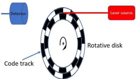
A rotary encoder is a sensor composed of a light source, photodetector and rotation disk with a code track, which translates rotation position into digital pulse signals, figure2.6. The code track in the rotation disk is composed of opaque and transparent sectors. As the disk rotates these patterns block the light from arriving at the photodetector, thus creating digital pulses as shown in figure2.7
This type of device cannot provide absolute position, but it can offer a high resolution approximation by using two output channels to sense position. These two code tracks in the rotation disk are composed of patterns 90◦ out of phase allowing not only high resolution positioning of the rotation disk but also its direction. Considering channel A and B, as shown in figure2.7, if A leads B then the disk is rotating counterclockwise, if not then clockwise.
The encoders can be divided in three types:
x1 encoding - The encoder counts movement by detecting only rising edges or only falling edges of channel A. Channel B is used to detect the rotation direction.
C H A P T E R 2 . T H E O R E T I CA L BAC KG R O U N D
Figure 2.6: Schematic representation of the working principal of an optical incremental rotary encoder.
Figure 2.7: Schematic representation of the working principal of an optical incremental rotary encoder.
x4 encoding - The encoder counts movement by detecting both rising and falling edges of both A and B channels. This type of encoder has highest resolution.
Most encoders also include another feature called the reference signal (MKP), which sends a digital pulse signal for every full rotation of the rotation disk.
2.6 Di
ff
erential signaling
Differential signaling is a technique which offers high immunity against electromagnetic impact in transmission lines. This technique, as shown in figure2.8, transmits informa-tion via two complementary or differential pair signals.
These signals are commonly transmitted in twisted pair cables, so noise affects both transmission lines identically. When both signals arrive a differential receiver unit, the noise is removed leaving the signal intact.
2 . 6 . D I F F E R E N T I A L S I G N A L I N G
C
h
a
p
t
e
r
3
E x p e r i m e n ta l Se t u p
In this chapter the experimental setup used to achieve a single diameter measurement will be shown and explained in four parts: mechanical setup, the optical setup, digital data analyzes and measurement results.
The optical setup will describe the used optical components, mathematical analyses and laser beam pathway in order to measure displacement, while in the mechanical setup the designs of the vacuum chamber, SPM support and reference mirrors are explained. In the digital analyzes section, demonstrates how the displacement is calculated and how a circumference map of the SPM is achieved. Lastly the measurement results are shown.
3.1 Mechanical setup
In figure3.1are shown the components mentioned in the previous section in their physi-cal form inside the vacuum chamber which operates at a pressure ofpvacuum≈50−100 mbar . The aluminum chassis IFO1 and IFO2, contains the optic components necessary to measure the displacement in the surface of the SPM. The spherical lenses used to focus the beam on the surface of the SPM are mounted on adjustable three-axial linear stages.
3.1.1 Spherical proof mass support and reference mirrors support
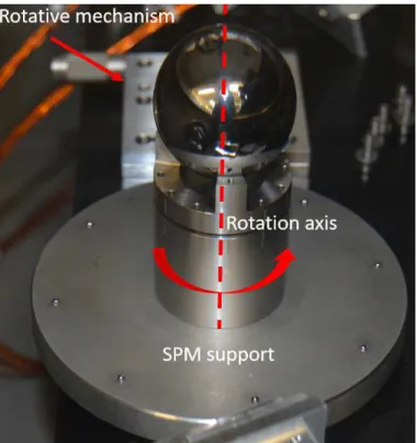
The SPM support is fixed to the rotational stage with a spring ring over the little spheres in the base plate, so it rotates as the rotational stage rotates with the rotation axis and direction indicated in figure3.2. Also in the figure, a rotative mechanism is present which allows for a shift in the initial angle position of the SPM.
C H A P T E R 3 . E X P E R I M E N TA L S E T U P
Figure 3.1: Vacuum chamber with double interferometers (IFO1 and IFO2) and SPM in the center[17]
Table 3.1: SPM properties[18]
Parameters Dimension Nominal diameter 40 mm Max diameter deviation 11,5µm Max diameter fluctuation 0,5µm
Roughness 0,032µm
Mass 0,4963kg
The reference mirrors (RM1 and RM2) have the possibility of being oriented using flexure hinges and tiltable plate.
The SPM used to carry out this experiment is a commercially common tungsten car-bide ball used for large ball bearing, quality Class G20 according to DIN5401 with the parameters in table3.1.
3.2 Optical setup
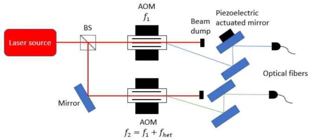
The experimental setup designed at Airbus D&S uses a double interferometer with het-erodyne frequency of 10 kHz, spatial separation of the different frequency beams and per-fect symmetry. The interferometers are fed by a Nd:YAG NPRO laser Innolight Mephisto NE500, at 1064 nm. The laser beam is split by a beam splitter originating two other
3 . 2 . O P T I CA L S E T U P
Figure 3.2: Rotation support for the SPM on top with the little support spheres in the base plate.
Figure 3.3: Reference mirrors support plate [17]
beams. These beams suffer a frequency shift by the AOMs, here is where heterodyne frequency of fhet = 10 kHz is established, figure3.4. After having defined two beams with different offset frequencies of 78.00 MHz and 78.01 MHz, these are transported via optical fibers to the vacuum chamber.
With the beams inside the vacuum chamber, figure3.5, the beamf1is detected by
PD1 and beamf2is detected byPD2. PD1andPD2are responsible for controlling the
intensity of the two beams via modulating the AOMs. Further along, each beam is yet again split in two other beams by a Koester prism, figure3.6. The beams with frequencyf1
C H A P T E R 3 . E X P E R I M E N TA L S E T U P
Figure 3.4: Simplistic schematic of the heterodyne frequency generation with spatial separation and symmetric design in use.
Figure 3.5: Inside the vacuum chamber with photodiodes (PD).
direction tilting, reaching a beam splitter and are redirected to the QPDs. The beams with frequencyf2hit a polarized beam splitter and then go through a quarter wave plate
circularly polarizing the beams. The same beams go through another system of AMs and are redirected to the surface of the SPM and reference mirrors. The measurement beam is focused on the surface of the SPM via plano-convex lens with a focal length of≈100 mm resulting in a measurement beam diameter at the SPM ofDmeas= 175µm. The beams are reflected back to the quarter wave plate, become linearly polarized again, and then reflected towards the beams of frequencyf1where they superimpose and are directed
towardsQPD1andQPD2. The signals detected by theQPDs are averaged over the beam
cross-section, thus resulting in a low pass filtering of the measured topography for spatial frequencies higher than 2
π. Dmeasor angular frequencies higher than 1.27◦. TheQPDs
3 . 3 . D I G I TA L DATA A N A LY Z E S
Figure 3.6: Beams are reflected back from the surface of the SPM and reference mirrors (RM), and it’s possible to calculate the displacement. PBS stands for polarized beam splitter, BS as in beam splitter, λ4 for quarter wave, KP is Koester prism, AM as adjustable mirrors and RS as rotational stage.
will detect the superimposed beam off1 andf2 and control the piezoelectric actuated
mirror to adjust the path length in figure3.4, adjusting thus the phase. The light intensity directed toQPD1, or reference QPD, is
Ir=Af1·Af2cos (∆ωt) (3.1)
and direct toQPD2, or measurement QPD, is
Im=Af1·Af2cos (∆ωt−∆φ(t)) (3.2)
In the equations3.1and3.2,Af1is the amplitude of the beam with frequencyf1,Af2is
the amplitude of the beam with frequencyf2,∆ωis the heterodyne frequency and∆φ(t)
is the phase difference between the measurement and reference signals.
3.3 Digital data analyzes
3.3.1 Field Programmable Gate Array
C H A P T E R 3 . E X P E R I M E N TA L S E T U P
Figure 3.7: FPGA board and host signal analysis.
The FPGA used in this experimental setup is a PXI RIO 7854R from National instru-ments, with a maximum data processing speed or single cycle loop speed of 40 MHz.
Both the FPGA and host are coded in LabVIEW.
From the QPDs, eight signals are obtained, figure 3.7. These signals in the FPGA board are divided in two identical signals to do an in-quadrature measurement, at a speed of 160 kHz. An in-quadrature consists in multiplying two identical signals with two other signals internally generated by the FPGA board, in all equal but with a 90° phase shift relative to each other.
In the FPGA board, these signals are obtained:
S1=Im·cos (∆ωt) =Af1·Af2·cos (∆ωt−∆φ(t))·cos (∆ωt)
S2=Im·sin (∆ωt) =Af1·Af2·cos (∆ωt−∆φ(t))·sin (∆ωt)
(3.3)
To the equations above, a low pass filter with a cut-offfrequency of 6 Hz is applied to filter out the high frequency part thus, resulting in
S1=12Af1·Af2·cos (∆φ(t))
S2=12Af1·Af2·sin (∆φ(t))
(3.4)
After the signals are low pass filtered, these are stored in aFirst in first out (FIFO)
memory at a frequency of 20 Hz.
3.3.2 Host program
The host program in the workstation, removes the data from the FIFO at a maximum speed of 20Hzand proceeds with the calculation of the phase signal, which is given by
φ(t) = arctan S2 S1 !
(3.5)
3 . 4 . M E A S U R E M E N T R E S U LT S
Since the phase difference between the measurement signal and the reference signal is directly proportional to the displacement, the following equation can be derived
∆φ(t) =4πn
λ ∆l(t) (3.6)
wherenis the refractive index of the medium in which the light travels and theλis the wavelength of the used laser beam.
As the host program calculates the displacement values, it also records the correspond-ing angular position. This angular position is obtained via ethernet connection between the host program and the rotational stage encoder. Thus resulting in a map of a single circumference of the SPM.
3.4 Measurement results
With the described setup, various systematic and stochastic noise sources have to be taken into consideration for the possibility to map topographically a single circumference of the SPM. Such noise sources are:
• Mechanical and thermal deformations in the setup.
• Radial and axial error movements of the SPM.
• Eccentricity of the rotation axis.
3.4.1 Noise Sources
In order to study if the measurement of the SPM topography is invalidated due to per-formance and accuracy issues caused by mechanical and thermal deformations in the system, a test measurement was done with the SPM static (no rotation motion).
As seen in the figure3.8, the effects of thermal and mechanical noise in this experi-mental setup are neglectable due to the picometer noise displacement for 10−3−100Hz frequencies and few nanometer displacement for frequencies lower than 10−3Hz.
These results prove that mechanical and thermal fluctuations are not limiting factors in the measurements.
The model of correction used is shown in figure3.9. In this modelCIFOis the center position of measurement between both interferometers,CSPM is the geometric center of mass of the SPM,x1and−x2are the measurement signals of each interferometer where the
negative sign ofx2comes in opposition to the measurement direction ofx1, misalignment
of the rotational stage generates→−c which is a static offset between the rotation axis and reference frame,→−s is the dynamic radial and axial error movements of the rotation axis due to ball bearing in the rotational stage,→−d represents the eccentricity caused by the offset between rotation axis and SPM geometric center,→−m is the position of theC
C H A P T E R 3 . E X P E R I M E N TA L S E T U P
Figure 3.8: Mechanical and thermal noise displacement evaluation, showing a high sym-metry of the two interferometers and the neglectable effect of these disturbances in the measurements.[17]
Figure 3.9: Schematic model of the geometry.[17]
The component→−m is calculated by
− →
m =→−c +→−s +→−d (3.7)
since the component→−s is composed of synchronous error movements, which repeat itself
3 . 4 . M E A S U R E M E N T R E S U LT S
every 2πinterval, and asynchronous error movements,→−m can be expressed as
− →
m(ϕ) =→−c +−→sse(ϕ) +−−→sae (ϕ) +→−d (ϕ) (3.8)
Asynchronous movement errors can be ignored if averaging of the measurements is
done and→−d (ϕ) =d→−ed(ϕ−ϕd) withd =
− → d and − →e
d(ϕ−ϕd) =
cos (ϕ−ϕd) sin (ϕ−ϕd)
0 , results in −
→m(ϕ) =→−c +−→s se (ϕ) +d
cos (ϕ−ϕd) sin (ϕ−ϕd)
0 (3.9)
Considering a sphere of radiusR
R2=h±x1,2(ϕ)−→ex − −→m(ϕ)
i2
(3.10)
the solutions are
x1,2(ϕ) =R s
1−m
2
y(ϕ) +m2z(ϕ)
R2 ±mx(ϕ) (3.11)
and describing the SPM surface ˆp(ϕ, θ) with spherical coordinates
R2= 1 4π π Z 0 2π Z 0 ˆ
p2(ϕ, θ) sin (θ)dϕdθ (3.12)
withθ=π2, results in
x1,2(ϕ, ϕSPM)≈pˆ
π
2 −ϕ±
π
2+ cy
R
+ϕSPM
s
1−m
2
y(ϕ) +m2z(ϕ)
R2 ±mx(ϕ) (3.13)
The equations3.13represent the measurement signals of the interferometers, in which dependencies exist from the misalignment between the rotational axis andCIFO, cy
R, and the relative rotation of the SPM enabled by the support,ϕSPM.
In table3.2are shown the error intervals of the parameters mentioned in the correc-tion model3.9for one rotation. The error margins of
→−c
,d and
→−s
are higher than the
surface topography error, therefore these errors have to be removed. In order to do so, measurements with several rotations were made. This allowed to remove the x-offset, cx= 0, by subtracting the mean values from the interferometer signals leaving the y-offset cy and eccentricityd. These two parameters can be estimated with a Taylor expansion of equation3.11, with scalar productξ1,2=
D
eiϕ
x1,2(ϕ)
E
C H A P T E R 3 . E X P E R I M E N TA L S E T U P
Table 3.2: Calculated error parameters for one rotation measurement
Parameters Error dimension
→−c
≈10−20µm
d ≈10−20µm
→−s
≈1−2µm
SPM surface topography ≈100 nm
ξ1,2=±
d 2e
i−ϕd±cyR
+dO c y R 2 (3.14) where
cy≈R2[arg (ξ1)−arg (ξ2)] ,
d≈ |ξ1|+|ξ2|,
ϕd ≈ −arg (ξ1−ξ2) .
(3.15)
From here corrected interferometer signalsxc1,2can be calculated
x1c,2=x1,2(ϕ, ϕSPM)∓dcos (ϕ−ϕSPM) +
h
cy+dcos (ϕ−ϕSPM)i2
2R (3.16)
In equation3.16the parametersd andϕd, which are errors of eccentricity caused by an offset between the rotation axis andCSPM, have to be calculated for each measurement due to random variations of their value because of the lash suffered by the SPM support. The parametercyalso suffers slight variations but these are due to thermal drifts caused by long measurement times which influence beam alignment and SPM position.
In previous calculations the influence of error movements by the rotational stage were ignored. Taking these error into consideration, the→−s component is calculated by removing the surface topographic contributions of the SPM from the measurement data with different initial angleϕSPM, resulting in
sx(ϕ)≈ x c
1(ϕ,0)−xc2(ϕ,0) +xc1(ϕ, π)−xc2(ϕ, π)
4 (3.17)
and
σ(ϕ) =sy(ϕ)cy+sz(ϕ)cz
R (3.18)
In order to estimate the value ofσ(ϕ) using the equation3.17resulted in a hard to solve ambiguity, hence a solution without high frequency content is used, resulting in
p1,2(ϕ, ϕSPM) = ˆp1,2(ϕ, ϕSPM)−R≈x1c,2(ϕ, ϕSPM)∓sx(ϕ) +σ(ϕ) (3.19)

![Figure 1.4: Visual representation of the acquired data. Figure taken from Abbot et al., PRL 116, 061102 (2016)[2]](https://thumb-eu.123doks.com/thumbv2/123dok_br/16545911.736929/25.892.248.660.151.499/figure-visual-representation-acquired-data-figure-taken-abbot.webp)

![Figure 3.1: Vacuum chamber with double interferometers (IFO1 and IFO2) and SPM in the center[17]](https://thumb-eu.123doks.com/thumbv2/123dok_br/16545911.736929/44.892.137.756.149.578/figure-vacuum-chamber-double-interferometers-ifo-ifo-center.webp)
![Figure 3.10: Measurement of the SPM surface on the top, p 1 , and deviation on the bottom, ǫ R .[17]](https://thumb-eu.123doks.com/thumbv2/123dok_br/16545911.736929/53.892.254.635.397.672/figure-measurement-spm-surface-p-deviation-ǫ-r.webp)
![Figure 3.11: Measurement of the average SPM surface in polar coordinates exaggerated by a factor of ≈ 10 4 between R and the topographical e ff ects.[17]](https://thumb-eu.123doks.com/thumbv2/123dok_br/16545911.736929/54.892.289.606.214.553/figure-measurement-average-surface-coordinates-exaggerated-factor-topographical.webp)

