A coherent approach to non-integer order derivatives

Signal Processing 86 (2006) 2505–2515

A coherent approach to non-integer order derivatives

Manuel Duarte Ortigueira

,1

UNINOVA, Campus da FCT da UNL, Quinta da Torre, 2825-114 Monte da Caparica, Portugal

Received 5 May 2005; received in revised form 7 December 2005 Available online 2 March 2006

Abstract

The relation showing that the Gru¨nwald-Letnikov and generalised Cauchy derivatives are equal is presented. This establishes a bridge between two different formulations and simultaneously between the classic integer order derivatives and the fractional ones. Starting from the generalised Cauchy derivative formula, new relations are obtained, namely a regularised version that makes the concept of pseudo-function appear naturally without the need for a rejection of any infinite part. From the regularised derivative, new formulations are deduced and specialised first for the real functions and afterwards for functions with Laplace transforms obtaining the definitions proposed by Liouville. With these tools suitable definitions of fractional linear systems are obtained.

r2006 Elsevier B.V. All rights reserved.

Keywords:Fractional difference; Fractional derivative; Fractional linear system; Differintegrator

1. Introduction

Fractional calculus, while over 300 years old, is still a young field, rich in opportunities for fundamental discoveries. In recent years fractional calculus has been rediscovered by scientists and engineers and applied in an increasing number of fields, namely in the areas of electromagnetism, control engineering, and signal processing. The increase in the number of physical and engineering processes that are best described by fractional differential equations has motivated out its study. This led to an enrichment of fractional calculus with

new approaches that however brought contribu-tions to a somehow chaotic state of the art. In fact, there are several definitions that lead to different results, making difficult the establishment of a systematic theory of fractional linear systems in agreement with the current practice. Riemann– Liouville, Caputo, Gru¨nwald-Letnikov, Hadamard, Marchaud, are some of the known definitions

[1–9,16,17]. Although from a purely mathematical point of view it is legitimate to accept and even use one or all, from the point of view of applications the situation is different. In our case of signal proces-sing applications, we should accept only the definitions that might lead to a fractional systems theory coherent with the usual practice, and accepted notions and concepts such as the impulse response and transfer function. In previous papers

[7–9]we made some contributions toward this goal;

www.elsevier.com/locate/sigpro

0165-1684/$ - see front matterr2006 Elsevier B.V. All rights reserved. doi:10.1016/j.sigpro.2006.02.002

_{Tel.: +351 1 2948520; fax: +351 1 2957786.}

E-mail addresses:mdortigueira@uninova.pt, mdo@dee.fct.unl.pt.

1_{Also with INESC_ID, R. Alves Redol, 9, 2}

however, despite these developments, several topics remained without a clear and concise formulation, namely and surprisingly, the definition of fractional derivative2 suitable for our interests. In [9] we addressed this problem and proposed a solution based on a reasoning that led to the use of the Gru¨nwald-Letnikov and the so-called generalised functions (Cauchy), forward and backward deriva-tives.3These choices were motivated by four main reasons: they do not need superfluous derivative computations, do not insert unwanted initial con-ditions, are more flexible and allow sequential computations. However, in this earlier approach we did not present a coherent mathematical reason-ing or a connection between the two formulations. In this paper, we propose to provide these missing links. In facing this problem, we assume as a starting point the definitions of direct and reverse fractional differences and their integral representa-tions[11–13]. From these representations and using the asymptotic properties of the Gamma function, we obtained in[12,13]a generalised Cauchy integral as a unified formulation for any order derivative. As we proved in[12,13]:

The generalised Cauchy derivative is equal to the Gru¨nwald-Letnikov fractional derivative.

When trying to compute the Cauchy integral using the Hankel contour we conclude that:

the integral has two terms: one corresponds to a derivative and the other to a primitive,

the exact computation leads to a regularised integral, generalising the well-known concept of pseudo-function, but without rejecting any in-finite part,

the definition implies causality.

The forward and backward derivatives emerge here as very special cases. We will study them for the case of functions with Laplace transforms. This leads us to define a causal and an anti-causal fractional linear differintegrators both with transfer function equal to sa_{;a2R, and to compute their} corresponding impulse responses.

The paper outline is as follows. In Section 2, we present the way we followed from the fractional differences to the fractional derivative defined in the complex plane, obtaining the well-known Cauchy integral. The analysis of the generalised Cauchy integral is done in Section 3 with the help of the Hankel contour. We present a general formula and two special cases valid for real variable functions. We exemplify with the exponential function and present the forward and backward derivatives as special cases valid for real functions in Section 4. In Section 5, we treat the case of functions with Laplace transform and obtain the formulae we named before by Cauchy differintegrations [9], but that must be named as Liouville differintegrations, since they were proposed first by Liouville [10]. These are suitable for fractional signals and systems studies [7] since they allow a generalisation of known concepts without meaningful changes as shown in Section 6. In Section 7 we will present some conclusions. At last in Appendix we obtain the impulse response for the differintegrator defined as a linear system with transfer function equal to

sa_;a2R.

Caution: In this paper we deal with a multivalued expressionza. As is well known, to define a function we have to fix a branch cut line and choose a branch (Riemann surface). It is a common procedure to choose the negative real half-axis as branch cut line. In what follows we will assume that we adopt the principal branch and assume that the obtained function is continuous above the branch cut line. With this, we will write ð1Þa¼ejap_.

2. From differences to derivatives

2.1. Difference definitions

Let fðzÞ be a complex variable function and introduceDdandDras finite ‘‘direct’’ and ‘‘reverse’’ [12,13]order one differences defined by

DdfðzÞ ¼fðzÞ fðzhÞ (1)

and

DrfðzÞ ¼fðzþhÞ fðzÞ (2)

with h2C and we assume that ReðhÞ40. For any

order (including the negative integer case) we have

[9,11]:

Da_dfðzÞ ¼X

1

k¼0

ð1Þk a

k

fðzkhÞ (3)

2_{Here we will speak mainly in terms of the fractional or}

non-integer order derivative, avoiding the use of fractional integral, because the calculus of the derivative may be done through an integral. So the word integral would appear with two different assertions. We will use derivative of negative order or primitive.

3_{As pointed out by Dugowson[10]these were already proposed}

and

Da_rfðzÞ ¼ ð1ÞaX

1

k¼0

ð1Þk a

k

fðzþkhÞ, (4)

where a_k

are the binomial coefficients.

2.2. On the Gru¨nwald-Letnikov differintegrations

Divide (3) by ha to obtain the fractional incre-mental ratio. Performing the computation of its limit as h!0þ,4 we obtain the direct Gru¨nwald-Letnikov derivative given by

Da_dfðzÞ ¼ lim

h!0þ P1

k¼0ð1Þ k a

k

fðzkhÞ

ha , (5)

where h is any complex number in the right-hand complex plane. Making a substitution h! h

for usingð4Þg, we obtain the reverse Gru¨nwald-Letnikov derivative:

Da_rfðzÞ ¼ lim

h!0þð1Þ

a

P1 k¼0ð1Þ

k a k

fðzþkhÞ

ha .

(6)

Expression (5) corresponds to the so-called left-hand sided Gru¨nwald-Letnikov fractional deriva-tive [15,16] while (6) has the extra factor ð1Þa, when compared with the right-hand sided Gru¨n-wald-Letnikov fractional derivative [10]. We main-tain that this factor must be remain-tained and continue to call the pairs defined by (5) and (6) as Gru¨nwald-Letnikov fractional derivatives. It is interesting to remark that these definitions were proposed first by Liouville[10].

Although we are not concerned here with existence problems, we must refer that in general we can have the direct derivative without existence of the reverse one and vice versa. For example, let us apply both definitions to the function fðzÞ ¼eaz. If

ReðaÞ4_{0, expression (5) converges to D}a dfðzÞ ¼ aa_eaz_{, while (6) diverges. On the other hand, if} fðzÞ ¼eaz _{Eq. (5) diverges while (6) converges to} Da

rfðzÞ ¼ ðaÞ

a_eaz_{. This suggests that (5) and (6)}

should be adopted for right and left functions,5 respectively, in agreement with Liouville reasoning

[10]. In particular, they should be used for the

functions such thatfðzÞ ¼0 forReðzÞo0 andfðzÞ ¼

0 for ReðzÞ40, respectively. It is interesting to

remark that, ifzandhare real, in (5) we are using the current and past values of the function: it is a

causal derivative; on the other hand, in (6) we use the current and future values: it is an anti-causal derivative.

2.3. Integral representations for the differences

Assume that fðzÞ is analytic inside and on an infinite integration path that encircles the pointst¼

zkh in the direct case and t¼zþkh in the corresponding reverse case, withk2Zþ

0. The results

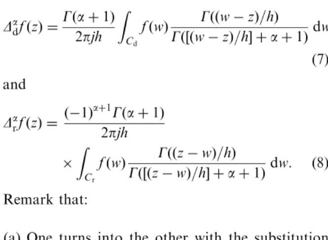
stated in (3) and (4) can be interpreted in terms of the residue theorem and written as[11–13]

Da_dfðzÞ ¼Gðaþ1Þ

2pjh Z

Cd

fðwÞ GððwzÞ=hÞ

Gð½ðwzÞ=h þaþ1Þdw

(7)

and

Da_rfðzÞ ¼ ð1Þ

aþ1_Gðaþ1Þ

2pjh

Z

Cr

fðwÞ GððzwÞ=hÞ

Gð½ðzwÞ=h þaþ1Þdw. ð8Þ

Remark that:

(a) One turns into the other with the substitution

h! h, as expected.

x x

x x

x

x

x x

x z

z+h z+2h

z+3h z+nh

z-h

z-2h

z-3h

z-nh

C_d

C

r

Fig. 1. Integration paths and poles for the integral representation of fractional order differences.

4₀þ_{means thatReðhÞ}4_0.

5_{We say that fðtÞ is a right [left] function if fð1Þ ¼0}

(b) The integration path must encircle the half-straight line that contains all the poles. This can be done with a U shaped contour like those shown inFig. 1.

(c) The direct and reverse differences are not equal.

2.4. Generalising the Cauchy formula

The ratio of two gamma functions ðGðsþ

aÞÞ=ðGðsþbÞÞhas the expansion[14,15]:

GðsþaÞ

GðsþbÞ¼s

ab _1þXN 1

ckskþOðsN1Þ

" #

(9)

asjsj ! 1, uniformly in every sector that excludes the negative real half-axis. As shown in[12]we can use the above expansion to obtain for the fractional incremental ratios the following representations:

Da_dfðzÞ

ha ¼

Gðaþ1Þ

2pj Z

Cd

fðwÞ 1

ðwzÞaþ1 dwþh:g1ðhÞ

(10)

and

Da_rfðzÞ

ha ¼

Gðaþ1Þ

2pj Z

Cr

fðwÞ 1

ðwzÞaþ1 dwþh:g2ðhÞ,

(11)

where g1ðhÞ and g2ðhÞ remain finite when h

decreases. Allowing h!0þ, we obtain the direct and reverse generalised Cauchy integrals:

Da_dfðzÞ ¼Gðaþ1Þ

2pj Z

Cd

fðwÞ 1

ðwzÞaþ1dw (12)

and

Da_rfðzÞ ¼Gðaþ1Þ

2pj Z

Cr

fðwÞ 1

ðwzÞaþ1 dw, (13)

that represent theaorder derivative. Whena¼N(a positive integer), both the derivatives are equal and coincide with the usual Cauchy derivative. In the fractional case we have different solutions, since we are using a different integration path. We can then define a generalised Cauchy integral by

DafðzÞ ¼Gðaþ1Þ

2pj Z

C

fðwÞ 1

ðwzÞaþ1 dw, (14)

whereC is any U shaped contour that encircles the half-straight line starting atzthat is the branch cut line of wa1_{. This formula has been used in}

fractional calculus [4,15,16] for defining what Campos calls the Liouville system[1]. Some authors use a different version for branched functions that

uses a closed integration path: it is the called Riemann system [1,2,15]. According to the theory we just developed this way of introducing deriva-tives does not conform to the assumptions behind (14). So, it does not lead to valid derivatives: it results in what we call pseudo-derivatives. In applying (14) to a branched function, the integra-tion path must be inside the analyticity domain of the function. This means that the branch cut line used in (14) cannot cut any other branch cut lines used to define the function.

3. Analysis of Cauchy formula

Consider the generalised Cauchy formula (14) and rewrite it in a more convenient format obtained by a simple translation:

DafðzÞ ¼Gðaþ1Þ

2pj Z

C

fðwþzÞ 1

waþ1 dw, (15)

where we assume that fðzÞ is analytic in a region that contains the contourC. Here we will chooseC

as a special integration path: the Hankel contour represented in Fig. 2. We assume that it surrounds the selected branch cut line. This is described by

x:ejy_{, with x2R}þ _{and y2 ½0;2pÞ. The circle has a}

radius equal to r small enough to allow it to stay inside the region of analyticity of fðzÞ.

With this contour, we can decompose (15) into three integrals along the two half-straight lines and the circle. It is interesting to remark that if a is a positive integer, the integrals along the straight lines cancel out and it remains the integral over the

C₁

C₂

C₃

circle: we obtain the usual Cauchy formula. Ifais a negative integer, the integral along the circle is zero and we are led to the well-known repeated integration formula[3,4,15,16]. In the generalacase we need the two terms. Let us decompose the above integral using the Hankel contour. For reducing steps, we will assume already that the straight lines are infinitely near to each other. We have, then:

DafðzÞ ¼ Gðaþ1Þ

2pj Z

C1

þ

Z

C2

þ

Z

C3

fðwþzÞ 1

waþ1 dw. ð16Þ

Over C1 we have w¼x:ejðy2pÞ, while over C3 we

have w¼x:ejy_{, with x2R}þ_{; over C}

2 we have w¼rejj_{, withj2 ðy2p;yÞ. We can write, at last:}

DafðzÞ ¼ Gðaþ1Þ

2pj

Z r

1

fðx:ejðy2pÞ_þzÞejaðy2pÞ xaþ1 dx

þ

Z 1

r

fðx:ejy_þzÞejay

xaþ1 dx

þGðaþ1Þ

2pj

1 ra

Z y

y2p

fðr:ejjþzÞ

ejajjdj. ð17Þ

For the first term, we have:

Z r

1

fðx:ejðy2pÞ_þzÞejaðy2pÞ xaþ1 dx

þ

Z 1

r

fðx:ejyþzÞe

jay

xaþ1 dx

¼ ½ejaðy2pÞþejay

Z 1

r

fðx:ejy_þzÞ 1

xaþ1 dx

¼ejay_½1ej2pa

Z 1

r

fðx:ejy_þzÞ 1

xaþ1 dx

¼ ejaðpyÞ:2jsinðapÞ

Z 1

r

fðx:ejy_þzÞ 1

xaþ1 dx, ð18Þ

where we assumed that fðx:ejðy2pÞ_{þzÞ ¼} fðx:ejy_{þzÞ, becausefðzÞis analytic.}

For the second term, we begin by noting that the analyticity of the functionfðzÞallows us to write:

fðx:ejy_{þzÞ ¼}X1 0

fðnÞðzÞ

n! x

n_ejny ₍₁₉₎

forxor2Rþ. We have, then:

j 1

ra

Z y

y2p

fðr:ejjþzÞejajdj

¼j 1

ra

X1

0

fðnÞðzÞ

n! r nZ y

y2p

ejðnaÞj_{dj. ð20Þ}

Performing the integration, we have:

j 1

ra

Z y

y2p

fðr:ejjþzÞejajdj

¼ j:ejapX1 0

fðnÞðzÞ

n! r

na_ejðnaÞy2:sin½ðnaÞp

ðnaÞ

¼ 2j:ejap_sinðapÞX1 0

fðnÞðzÞ

n!

ejðnaÞy_rna

ðnaÞ . ð21Þ

But the summation in the last expression can be written in another interesting format:

X1

0 fðnÞðzÞ

n! :

ejðnaÞy_rna

ðnaÞ

¼ X

N

0 fðnÞðzÞ

n! e jnyZ 1

r

xna1dx

þX

1

Nþ1 fðnÞðzÞ

n!

ejny_rna

ðnaÞ,

whereN¼ bac.6Substituting it in (21) and joining to (18) we can write:

DafðzÞ ¼K:

Z 1

r

fðx:ejy_þzÞ PN 0

fðnÞðzÞ

n! e jny_xn

" #

xaþ1 dx

K:X 1

Nþ1

fðnÞðzÞ

n! ð1Þ n rna

ðnaÞ. ð22Þ

Ifao0, we make the inner summation equal to zero.

Using the reflection formula of the gamma function we obtain forK:

K¼ Gðaþ1Þe

jðpyÞa

p sinðapÞ ¼ ejðpyÞa

GðaÞ. (23)

Now let r go to zero. The second term on the right-hand side in (22) goes to zero and we obtain:

DafðzÞ ¼ e

jðpyÞa

GðaÞ

Z 1

0

fðx:ejy_þzÞ PN 0

fðnÞðzÞ

n! e jny_xn

" #

xaþ1 dx,

ð24Þ

that is valid for anya2R. It is interesting to remark that (24) is nothing else but a generalisation of the ‘‘pseudo-function’’ notion [17], but valid for an analytic function in a non-compact region of the complex plane. Relation (24) represents a regu-larised fractional derivative that has some simila-rities with the Marchaud derivative [15]: for 0oao1, they are equal. A special case of (24), for

y¼p, can be found in [15]. It was obtained using the concept of finite part Hadamard integral. However, (24) appears naturally from the general-ised Cauchy derivative without having to reject any infinite part.

If one putsw¼x:ejy_{, we can write:}

DafðzÞ ¼ 1

GðaÞe

jpa

Z

g

fðwþzÞ PN 0

fðnÞðzÞ

n! w n

" #

waþ1 dw,

ð25Þ

wheregis a half-straight line starting atw¼0. As we can conclude there are infinitely many ways of computing the derivative of a given function: these are defined by the chosen branch cut lines. However, this does not mean that we have infinitely many different derivatives. It is not hard to see that all the branch cut lines belonging to a given region of analyticity of the function are equivalent and lead to the same result unless the integral may be divergent if the function increases without bound. The results just obtained assume that fðzÞ

is analytic in the region inside and on the integration path. If we are dealing with functions with poles or branch points, these must be excluded from that region.

4. Examples

4.1. The exponential function

To illustrate the previous assertions we are going to consider the case of the exponential function. Let

fðzÞ ¼eaz_{, with a2R}þ_{. Inserting it into (24), it}

becomes

DafðzÞ ¼ 1

GðaÞe

jðpyÞa_eaz

Z 1

0

½eax:ejyPN 0 a

n n!e

jny_xn

xaþ1 dx. ð26Þ

With a variable change t¼ axejy_{, the above} equation gives:

DafðzÞ ¼ 1

GðaÞa

a eaz

Z 1:aejy

0

½etPN 0 ð1Þ

n n! tn taþ1 dt,

(27)

where the integration path is half-straight line that forms an angle equal toywith the positive real axis. The integral in (27) is almost the generalised Gamma function definition presented in[18]and is a generalisation of Euler integral representation for the gamma function. But this requires integration along the positive real axis. However, as shown in

[14]the integration can be done along a ray with an angle in the interval 0;p=2½. This implies that we must haveReðaejy_{Þ40. We have then:}

a40 cosðyÞo0; ao0 cosðyÞ40: (

This means that if a40, the branch cut line must

belong to left-hand half-plane; while if a40, the

branch cut line must belong to right-hand half-plane. As the integrand is analytic outside the branch cut line, we can integrate along the positive real axis. So, we can write:

DafðzÞ ¼ 1

GðaÞa

a_eazZ 1

0

½etPN 0

ð1Þn n! t

n

taþ1 dt.

(28)

The integral defines the value of the gamma function GðaÞ [18] if we maintain the convention made before: whenao0 the summation is zero. We

then obtain:

Daeaz¼aaeaz (29)

as expected. In a particular limiting case,a!0, we obtain Da1¼0 if a40. If ao0, it is infinite. The

the same conclusions as seen. We must be careful in using (29). In fact, in a first glance, we could be led to use it to compute the derivatives of functions like sinðzÞ, cosðzÞ, sinhðzÞand coshðzÞ. But if we have in mind our reasoning we can conclude immediately that functions do not have finite derivatives ifz2C. In fact they use simultaneously the exponentials ez _{and e}z _{which derivatives cannot exist}

simulta-neously, as we just saw. However, we can conclude that functions expressed by Dirichlet series

fðtÞ ¼P1₀ akelkt _{with all the Reðl}

kÞ positive or all

negative have finite derivatives given by fðaÞðtÞ ¼

P1

0 akðlkÞaelkt. In particular functions with Laplace

transform with region of convergence in the right or left half-planes have fractional derivatives. We will return to this case in a later section.

Another interesting case is the cisoid fðtÞ ¼ejot_,

o2Rþ. Inserting it into (24) again, it becomes

DafðtÞ ¼ 1

GðaÞe

jðpyÞa_ejot

Z 1

0

½ejox:ejyPN 0

ðjoÞn n! e

jny_xn

xaþ1 dx. ð30Þ

Withy¼p=2,joejy ¼ oand we obtain easily

DafðtÞ ¼ ðjoÞaejot. (31)

It is not difficult to see that (31) remains valid if oo0. We only have to put y¼ p=2. We can

conclude then that:

DacosðotÞ ¼oacosðotþap=2Þ. (32)

For sinðotÞ, it is similar.

4.2. The power function

Let fðzÞ ¼zb_{, with b2R. If b4a, we conclude} immediately thatDa½zb_{defined for everyz2Cdoes} not exist, unlessa is a positive integer, because the integral in (24) is divergent for everyy2 ½0;2p½. This has an important consequence: we cannot compute the derivative of a given function by using its Taylor series and computing the derivative term-by-term.

Let us see what happens for other values ofband for z in half-plane regions. The branch cut line needed for the definition of the function must be chosen to be outside the integration region. This is equivalent to say that the two branch cut lines cannot intersect. To use (24) we compute the successive integer order derivatives of this function

that are given by

Dnzb¼ ð1ÞnðbÞ_nzbn. (33)

Now, we have

Dazb

¼e

jðpyÞa

GðaÞ

Z 1

0

½ðx:cjy_þzÞbPN 0

ð1Þn_ðbÞ nzbn n! e

jny_xn

xaþ1 dx.

ð34Þ

With a substitutiont¼x:ejy_{=z, we obtain:}

Dazb¼ e

jpa

GðaÞz

ba

Z 1ejy=z

0

½ð1þtÞbPN 0

ð1Þn_ðbÞ n n! t

n

taþ1 dt.

ð35Þ

To simplify the analysis, let us assume that y¼0 andz2Rþ_{. We obtain:}

Dazb¼ e

jpa

GðaÞz

baZ 1

0

½ð1þtÞbPN 0

ð1Þn_ðbÞ n n! t

n

taþ1 dt.

(36)

As shown in[5,6], the integral in (36) is a generalised version of the Beta functionBða;abÞ valid for a2Randbo0. We conclude then that

Dazb¼e

jpa_GðabÞ GðbÞ z

ba ₍₃₇₎

valid for any a and bo0 and for z2Rþ. Using

the procedure described in[14]for dealing with the gamma function, it is not hard to show that the above formula is valid forz2Cþ.

This means that we have to use a branch cut line in the left half-plane. If z2C, we choose y¼p and obtain the above result again. As one can be considered as an analytical continuation of the other, we can conclude that (37) is valid for bo0

and anya, but we should be careful with the choice of the branch cut line. Forb40, the integral in (36)

is divergent explaining the affirmation we did at the beginning of this section.

4.3. The derivatives of real functions

4.3.1. y¼0—reverse derivative

This corresponds to choosing the real positive half-axis as branch cut line. Substitutingy¼0 into (24), we have:

Da_rfðzÞ ¼ e

jpa

GðaÞ

Z 1

0

½fðxþzÞ PN 0

fðnÞðzÞ n! x

n

xaþ1 dx.

(38)

As this integral uses the right-hand values of the function, we will call this backward or reverse derivative in agreement with[9].

4.3.2. y¼p—direct derivative

This corresponds to choosing the real negative half-axis as branch cut line. Substitutingy¼pinto (24) and performing the changex! x, we have:

Da_dfðzÞ ¼ 1

GðaÞ

Z 1

0

½fðzxÞ PN 0

fðnÞ_ðzÞ n! ðxÞ

n

xaþ1 dx.

(39)

As this integral uses the left-hand values of the func-tion, we will call this forward or direct derivative again in agreement with Ortigueira et al.[9].

5. Derivatives of functions with Laplace and Fourier transforms

Consider now the special class of functions with Laplace transform (LT). LetfðtÞbe such a function and FðsÞ its LT7, with a suitable region of convergence,Rc. This means that we can write

fðtÞ ¼ 1

2pj Z aþj1

aj1

FðsÞestds, (40)

where a is a real number inside the region of convergence. Inserting (40) inside (38) and permut-ing the integration symbols, we obtain:

Da_rfðzÞ ¼ e

jpa

2pjGðaÞ

Z aþj1

aj1

FðsÞesz

Z 1

0

½esxPN 0

ðsxÞn n!

xaþ1 dxds. ð41Þ

If ReðsÞo0 and considering the result obtained in

Section 4.1 (see [14,18] also) the inner integral is equal to GðaÞ:sa_{; if ReðsÞ40 it is divergent. We} conclude that:

LT½Da_rfðtÞ ¼saFðsÞ forReðsÞo0. (42)

This means that there must exist an operator with transfer function equal to

FðsÞ ¼sa forReðsÞo0. (43)

This is an anti-causal operator with an impulse response equal to[7]

dð_raÞðtÞ ¼ t

a1_uðtÞ

GðaÞ , (44)

whereuðtÞis the Heaviside unit step. For the direct case, we use (39) and (40) to obtain again:

Da_dfðzÞ ¼ 1

2pjGðaÞ

Z aþj1

aj1

FðsÞesz

Z 1

0

½esxPN 0

ðsxÞn n!

xaþ1 dxds. ð45Þ

IfReðsÞ4_{0, the inner integral is equal toGðaÞ}:_sa_{; if}

ReðsÞo0 it is divergent. We conclude that:

LT½Da_dfðtÞ ¼saFðsÞ forReðsÞ40. (46)

Again there must exist an operator with transfer function equal to

FðsÞ ¼sa forReðsÞ40 (47)

and so, it is a causal operator with an impulse response equal to

dð_daÞðtÞ ¼t

a1_uðtÞ

GðaÞ . (48)

In Appendix we present the procedure for comput-ing the inverse LT of sa_{. With this formulation} we can conclude that we have a causal (forward) derivative that is the convolution of fðtÞ and dð_daÞðtÞ:

Da_dfðtÞ ¼ 1

GðaÞ

Z 1

0

fðttÞ:ta1_{dt (49)}

valid for functions with LT converging in a region that includes the right-hand side of the complex plane. Similarly, we have an anti-causal (backward) derivative valid for functions with LT converging in a region that includes the left-hand side of the complex plane and that is the convolution of fðtÞ

anddð_raÞ ðtÞ:

Da_rfðtÞ ¼ð1Þ

a

GðaÞ

Z 1

0

fðtþtÞ:ta1_{dt. (50)}

It is interesting to remark that these definitions were introduced both exactly with this format by Liou-ville [10]. Unhappily in the common literature the factorð1Þahas been removed. To give the correct

acknowledgement we will call (49) and (50) as Liouville forward and backward derivatives.8

To study the case of functions with Fourier transform, we can consider the results obtained in Section 4.1. However, we will use the derivatives just obtained. We begin by noting that the multi-valued expression FðsÞ ¼sa _{becomes an analytic} function as soon as we fix a branch cut line in all the complex plane excepting the branch cut line. The computation of the derivative of functions with Fourier transform is dependent on the way used to defineðjoÞa. If we define it doing the limit ass!jo from the right which means that

ðjoÞa¼ joja e

jap=2 _{if o40;}

ejap=2 _{if oo0;} (

(51)

we can use (46) and (49). If we perform the limit as

s!jofrom the left meaning that

ðjoÞa¼ joja e

jap=2 _{if o40;}

ej3ap=2 _{if oo0;} (

(52)

we are in the anti-causal case and use (43) and (50). The derivative expressed in (49) is equal to (5), we can somehow easily obtain a strange relation:

ta1uðtÞ

GðaÞ ¼hlim!0þ P1

k¼0ð1Þ k a

k

dðtkhÞ

ha . (53)

For the reverse case, we obtain a similar result.

6. Fractional linear systems

The results of the previous section are very important in applications since they allow us to introduce the useful concept of transfer function. In fact, if we define a linear system through a fractional differential equation with the general format:

XN

n¼0

anDnn_{yðtÞ ¼}X M

m¼0

bmDnm_{xðtÞ, (54)}

where the differentiation orders, nn, are, in the

general case, complex numbers. As usual, we apply the LT to Eq. (54) and use the results of Section 5, to obtain the transfer function of the system:

HðsÞ ¼

PM m¼0bmsnm PN

n¼0ansnn

(55)

with region of convergence defined by ReðsÞ40

(causal case) or ReðsÞo0 (anti-causal case). When

looking for the output,yðtÞ, to a given input,xðtÞ, we must consider the initial conditions. This is a problem that created much confusion and difficul-ties in the past [3,8,16] motivated by the use of several different derivative definitions and of the one-sided LT. In [8], we proposed a new way of looking at the problem. The proposed solution is based on the initial value theorem and on the Watson–Doetsch lemma:

The initial-value theorem Assume that jðtÞ is a causal signal such that in some neighbourhood of the origin is a regular distribution corresponding to an integrable function. Also,assume that there is a real number b41 such thatlim_t!0þjðtÞ=tb exists and

is a finite complex value. Then

lim

t!0þ

jðtÞ

tb ¼_slim_!1

sbþ1_FðsÞ

Gðbþ1Þ. (56)

For proof see[17].

Let us consider the class of functions with LT analytic forReðsÞ4_gthat verify

jðtÞ tb:X

1

n¼0

an t

nn_uðtÞ

Gðbþ1þnnÞ, (57)

as t!0þ where b41 and n40, where the

principal values of the powers are assumed n is greater than the maximum derivative order. The Watson–Doetsch lemma[14], states that the LTFðsÞ

ofjðtÞsatisfies:

FðsÞ 1

sbþ1 X1

n¼0 an 1

Snn (58)

ass! 1andReðsÞ40.

We will assume that the input and the output of the system described by (54) have the general format:

fðtÞ ¼X

L

n¼0

f_nðtÞtgn_{uðtÞ, (59)}

where 0og

nognþ1.L is a positive integer that may

be infinite, and the functions f_nðtÞ ðn¼0;. . ._;NÞ

and their derivatives of orders less than or equal to gN are assumed to be regular at t¼0. We may

assume them to be given by

f_nðtÞ ¼X

1

k¼0

ak t

kn_uðtÞ

Gðbþ1þknÞ. (60)

8_{The terms forward and backward are used here in agreement}

Let us introduce a sequenceb_n by

b_n¼g_nX

n1

k¼0

b_k; b₀ ¼g₀. (61)

The solution of the initial conditions problem is obtained through the substitution of each derivative in (54) by

jðgnÞ_{ðtÞ ¼ ½fðtÞ}:_uðtÞðgnÞX n1

i¼0

fðg_iÞð0þÞdðgngi1Þ d ðtÞ,

(62)

that states the general formulation of the initial value problem solution. As we can see, the initial values prolong their action for every t4_{0. This}

means that we have a memory about the initial conditions that decreases very slowly. Using the LT, we obtain:

LT½jðgnÞ_{ðtÞ ¼s}ðgnÞ_{FðsÞ s}gnX n1

i¼0

fðgiÞ_ð0þÞsgi1_,

(63)

that is a generalisation of the usual formula for introducing the initial condition. The sequence g_i ði¼0;1;. . ._{;nÞ is chosen accordingly to the}

following rules:

(a) Thennon the left (or right) side in (54) belong to

the sequence.

(b) The others are arbitrary unless the problem at hand suggests them.

(c) This means that we are almost free in choosing the intermediate derivatives between g_n and g_nþ1.

7. Conclusions

In this paper we proposed a new look at the fractional derivative by taking as starting point the Cauchy derivative formulation. We showed that it is equal to the Gru¨nwald-Letnikov and performed its analysis by using the Hankel contour. From this analysis we obtained a regularised formulation that we used to obtain special formulae as the forward and backward derivatives. These allowed us to obtain the original Liouville formulae valid for functions with LT. It is interesting to remark that the most common definitions used nowadays for fractional derivatives, e.g. Riemann-Liouville and Caputo do not enter into the developed scheme.

With this formulation we were able to introduce the fractional linear systems and the way out of introducing the initial conditions.

Appendix. Invertingsa

We are going to compute the Inverse LT ofsa_{, for} a2R. We assume the causal case with region of convergence defined by ReðsÞ40. Let da

dðtÞ be the

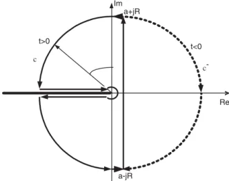
causal Laplace inverse transform of sa_{. By} simpli-city, we can choose the negative real half-axis as branch cut and constrain the argument of s to belong to the interval p;p. Consider the picture in Fig. 3.

For to0 we use the contour consisting of the

segment of straight line and the closing dotted half-circle. It is not hard to conclude thatda_dðtÞ ¼0. For

t4_{0 we use the bold integration path inFig. 3. This}

has 8 segments: the inversion straight line, two short parallel straight line segments, two quarter circles, two parallel long straight line segments and a small circle. The integral computed along the total contour, C, is null since in its interior the function is analytic. It is not difficult to show that the integrals along the circle arcs and along the short segments tend to zero asR! 1. For the integrals over the long segments it is not difficult to conclude that their sum is equal to 2jsinap:Rþ1

r xae

xt_dx,

r being the radius of the small circle. To compute the integral over the small circle we proceed as in Section 2.1. From the Taylor series for the exponential, we conclude that it equals

Im a+jR

Re

c

a-jR t>0

t<0

c-

2jsinðapÞ:P1₀ ðð1Þntnrnþaþ1ÞÞ=ðn!_{ðnþaþ1ÞÞ. If}

a is positive, the contribution of the small circle is zero as r goes to zero. If ao0, let N be the least

positive integer greater than jaj. In this case, the contribution is merely equal to

2jsinðapÞ:X

N

0

ð1Þntn_rnþaþ1 n!ðnþaþ1Þ

¼ 2jsinðapÞ:X

N

0

ð1Þntn n!

Z þ1

r

xnadx

Joining this expression to the above one and letting r go to zero, we obtain:

da_dðtÞ ¼2jsinpa

2pj : Z þ1

0

xa extð1Þ

n_ðtxÞn

n!

dx

The use of the definition and properties of the gamma function[18]leads immediately to (35). For

t¼0, the inversion integral is not convergent. However, its principal value is zero.

References

[1] L.M.C. Campos, On a concept of derivative of complex order with applications to special functions, IMA J. Appl. Math. 33 (1984) 109–133.

[2] L.M.C. Campos, Fractional calculus of analytic and branched functions, in: R.N. Kalia (Ed.), Recent Advances in Fractional Calculus, Global Publishing Company, 1993. [3] K.S. Miller, B. Ross, An Introduction to the Fractional

Calculus and Fractional Differential Equations, Wiley, New York, 1993.

[4] K. Nishimoto, Fractional Calculus, Descartes Press Co., Koriyama, 1989.

[5] M.D. Ortigueira, From differences to differintegrations, Fractional Calculus Appl. Anal., in preparation.

[6] M.D. Ortigueira, Two new integral formulae for the Beta function, Int. J. Appl. Math., in preparation.

[7] M.D. Ortigueira, Introduction to Fractional Signal Proces-sing. Part 1: Continuous-Time Systems, IEE Proc. Vision Image Signal Process. 1 (2000) 62–70.

[8] M.D. Ortigueira, On the initial conditions in continuous-time fractional linear systems, Signal Process. 83 (11) (November 2003) 2301–2309.

[9] M.D. Ortigueira, J.A. Tenreiro-Machado, J. e Sa´ da Costa, Which differintegrator?, IEE Proc. Vision Image Signal Process. 152 (6) (2005) 846–850.

[10] S. Dugowson, Les diffe´rentielles me´taphysiques, Ph.D. Thesis, Universite´ Paris Nord, 1994.

[11] J.B. Diaz, T.J. Osler, Differences of Fractional Order, Math. Comput. 28 (125) (January 1974).

[12] M.D. Ortigueira, Fractional differences integral representa-tion and its use to define fracrepresenta-tional differintegrarepresenta-tions, in: Proceedings of the ENOC-2005, Fifth EUROMECH Non-linear Dynamics Conference, Eindhoven University of Technology, The Netherlands, 7–12 August 2005.

[13] M.D. Ortigueira, A new look at the differintegration definition, in: Proceedings of the ENOC-2005, Fifth EUROMECH Nonlinear Dynamics Conference, Eindhoven University of Technology, The Netherlands, 7–12 August 2005.

[14] P. Henrici, in: Applied and Computational Complex Analysis, vol. 2, Wiley, New York, 1991, pp. 389–391. [15] S.G. Samko, A.A. Kilbas, O.I. Marichev, Fractional

Integrals and Derivatives—Theory and Applications, Gor-don and Breach Science Publishers, LonGor-don, 1987. [16] I. Podlubny, Fractional Differential Equations, Academic

Press, San Diego, 1999.

[17] A.H. Zemanian, Distribution Theory and Transform Ana-lysis, Dover Publications, New York, 1987.