MANUEL DUARTE ORTIGUEIRA
UNINOVA and Department of Electrical Engineering, Faculdade de Ciências e Tecnologia da Universidade Nova de Lisboa, Campus da FCT da UNL, Quinta da Torre, 2825 – 114 Monte da Caparica, Portugal ([email protected])
(Received 17 November 20051accepted 4 October 2006)
Abstract:Fractional central differences and derivatives are studied in this article. These are generalisations to real orders of the ordinary positive (even and odd) integer order differences and derivatives, and also coincide with the well known Riesz potentials. The coherence of these definitions is studied by applying the definitions to functions with Fourier transformable functions. Some properties of these derivatives are presented and particular cases studied.
Keywords: Fractional central difference, fractional central derivative, Grünwald-Letnikov, generalized Cauchy derivative
1. INTRODUCTION
In previous work (Ortigueira and Coito, 20041 Ortigueira, 2006a), we proposed a new ap-proach for introducing causal and anti-causal fractional derivatives based on four steps:
1. Use as a starting point the Grünwald-Letnikov forward and backward differences and derivatives.
2. With an integral formulation for the fractional differences, and using the asymptotic properties of the Gamma function, obtain the generalised Cauchy derivative.
3. Compute the integral defining the generalised Cauchy derivative, using the Hankel path to obtain regularised fractional derivatives.
4. Through application of these regularised derivatives to functions via the Laplace trans-form, the Liouville fractional derivative is obtained.
In other articles (Ortigueira, 2006b,c), we presented a similar procedure for central frac-tional derivatives. It comprises the following steps:
1. Introduction of the general framework for central differences, considering two cases, which we called type 1 and type 2. These are generalisations of the usual central differ-ences for even and odd positive orders respectively.
2. Limit computation, as for normal Grünwald-Letnikov derivatives.
3. Suitable integral representations for these differences were introduced. From these rep-resentations, we obtained the derivative integrals, using the properties of the Gamma
Journal of Vibration and Control,14(9–10):1255–1266, 2008 DOI: 10.1177/1077546307087453
1
function. The integration is performed over two infinite lines that “close at infinity” to form a closed path. Two generalisations of the usual Cauchy derivative definition are obtained, which agree with it when1 is an even or an odd positive integer, for type 1 and type 2, respectively.
4. The computation of these integrals over a path of two straight lines leads to generalisa-tions of the Riesz potentials.
The most interesting feature of the relations obtained lies in the summation formulae for the Riesz potentials.
In this article, we revise this procedure and test the coherence of the proposed frame-work, by applying them to the complex exponential. The results show that they are suitable for functions with Fourier transform. The formulation agrees also with the work of Okikiolu (1966). Special cases are studied, and some properties presented. The remainder of the arti-cle is arranged as follows: In section 2 we present the type 1 and type 2 central differences, and their integral representations. Central derivative definitions are presented in Section 3, and their integral representations obtained, generalising the Riesz potentials. In Section 4, we apply the definitions to the complex exponential to test the coherence of the definitions. The special integer order cases are studied, and some properties of the derivatives are presented. Finally, we present some conclusions.
2. FRACTIONAL CENTRAL DIFFERENCES AND THEIR INTEGRAL
REPRESENTATIONS
In this article, we consider two types of fractional central difference. In what follows,1 2
213h3 R4and f4t5is a complex variable function. We define a type 1 difference as
61
c1f4t55 46 1
26
4215k741415
741822k415741824k415f4t 2kh5 (1)
and a type 2 difference (for which we additionally assume that1is non-zero) is defined as
61c2f4t55 46 1
26
4215k741415f4t 2kh4h825
7[41415822k41]7[41215824k41]9 (2)
Using the relation (Andrews et al., 1999, p. 123)
46 1
26
1
74a2k41574b2k41574c4k41574d4k415
5 74a4b4c4d415
74a4c41574b4c41574a4d41574b4d415 (3)
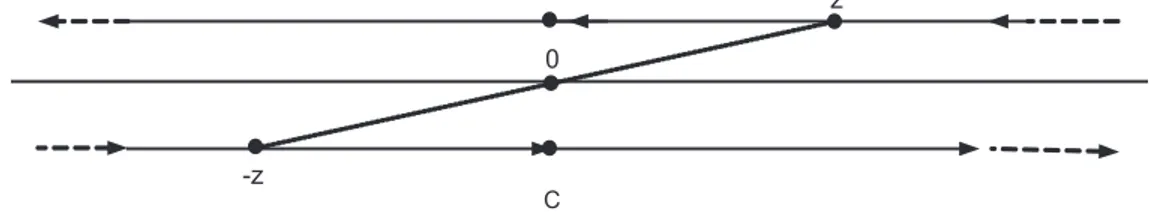
Figure 1. Integration path for integrals (11) and (12).
6c1
2
61c1f4t5
3
561c14f4t5 (4)
and
6c2261c2f4t535 2614
c1 f4t5 (5)
while
6
c2
2
61
c1f4t5
3
5614
c2 f4t5 (6)
provided that14 2 21. In particular, with14 5 0, relations (4) and (5) show that when 717 1 and 77 1 the inverse differences must exist, and can be obtained using formulae (1) and (2). It is worth noting that the zero order type 1 difference as obtained from equation (1)is the identity operator. The zero order type 2 difference will be considered later. Let us assume that f4z5 is analytic in a region of the complex plane that includes the real axis. To obtain integral representations for differences described above, we follow the procedure used by Ortigueira and Coito (Ortigueira and Coito, 20041Ortigueira, 2006a). We only need to give interpretations to (1) and (2) in terms of the residue theorem. Note that, for the first case, the poles must lie atnh,n3 Z. This leads easily to
61c1f4t55
741415
2j h
4
Cc
f4z4 5 7
5
2
h 41
6 7 5 2 h 4 1
2 41
6 77 h 8 77 h 4 1
2 41
8d 9 (7)
The integrand function has infinitely many poles at everynh, n 3 Z. The integration path must consist of infinite lines above and below the real axis, closing at infinity. The easiest example is obtained by considering two straight lines near the real axis, one above and the other below (see Figure 1). In the second case, the poles are located at half-integer multiples ofh, which leads to
61
c2f4t55
741415
2j h
4
Cc
f4z4 5 7 5 2 h 4 1 2 6 7 5 2 h 4 1
2 41
6 7 5 h 4 1 2 6 77 h 4 1
2 41
These integral formulations will be used in the next section to obtain the integral formulae for the central derivatives.
3. THE FRACTIONAL CENTRAL DERIVATIVES
To obtain fractional central derivatives we proceed as in previous cases (Samko et al., 19871 Ortigueira and Coito, 20041 Ortigueira, 2006a,b,c): Divide the fractional differences byh1
(h314) and leth 80. For the first case, and assuming again that1 221, we obtain
Dc1
1f4t5 5 limh80
61
c1f4t5
h1
5 lim
h80
741415 h1
46 1
26
4215k
741822k415741824k415f4t 2kh5 (9)
which we will call a type 1 fractional central derivative.
For the second case, and still additionally assuming that1 95 0, we obtain the type 2 fractional central derivative as
D1c2f4t5 5 lim
h80
61
c2f4t5
h1
5 lim
h80
741415 h1
46 1
26
4215kf4t 2kh4h825
7[41415822k41]7[41215824k41]9 (10)
Equations (9) and (10) generalise the positive integer order central derivatives to the fractional case, although there should be an extra factor, of 42151 82 in the first case and
42154141582in the second case, which we have removed.
To obtain the integral representations for the derivatives, we commute the limit and inte-gration in (7) and (8). To perform the limit computation inside the integral, we make use of the properties of the gamma function (Henrici, 1974). As shown previously (Ortigueira and Coito, 20041Ortigueira, 2006b,c), we obtain, for the type 1 case
Dc11f4t55 741415 2j
4
Cc
f4z45 1 4 518l 24142 5
182 r
d (11)
and, for the type 2 derivative
Dc12f4t55 741415 2j
4
Cc
f4z4 5 1 4 541l 41582425
4141582 r
The subscripts “l” and “r” indicate that the power functions have the left and right half real axis (respectively) as branch cut lines. Relations (11) and (12) are generalisations of the usual Cauchy formulae. Choosing a two straight line integration path as shown in Figure 1, we obtain for the type 1 derivative the expression
Dc11f4t55 1
274215cos41 825
6 4
26
f4z2x5 1
7x7141dx (13)
which is the so-called Riesz potential (Samko et al., 19871 Kilbas et al., 2006). Similarly, and as1is not an odd integer, we obtain for the second case
Dc1
2f4t55 2
1
274215sin41 825
6 4
26
f4z2x5sgn4x5
7x7141dx (14)
which is the modified Riesz potential (Samko et al., 1987). Both potentials (13) and (14) have been studied by Okikiolu (1966). These are essentially convolutions of a given function with two acausal (that is, neither causal nor anti-causal) operators, and are suitable for dealing with functions defined in1, and that are not necessarily equal to zero at6. In particular, they must be suitable for dealing with stationary stochastic processes (Ortigueira and Batista, 2006).
4. COHERENCE OF THE DEFINITIONS
4.1. Type 1 Derivative
We propose to test the coherence of the results by considering functions with Fourier trans-formable functions. To perform this study, we will examine the behaviour of the defined derivatives for f4t55e2jt,t, 31. In the following we will consider non-integer orders
greater than21. We start by considering the type 1 derivative. From (1) we obtain
61
c1e
jt
5e2jt 46 1
26
4215n741415
741822n415741824n415e
jnh
(15)
where we recognize the discrete-time Fourier transform of Rb4n5(which is, in purely
math-ematical terms a Fourier series with Rb4n5as coefficients), given by
Rb4n55
4215n741415
741822n415741824n4159 (16)
This function is the discrete autocorrelation of
hn 5
421825n
whereunis the discrete unit step Heaviside function (Ortigueira, 2000). As the discrete-time
Fourier transform ofhn is
H4ej55 F T[hn]5412e2jh5182 (18)
the discrete-time Fourier transform of Rb4n5is
S4ej5 5 lim
z8ejh412z
215182412z51825412e2jh
5182412ejh5182
5 99ejh822e2jh829915 72 sin4h825719 (19)
Thus,
72 sin4h82571 5 46 1
26
4215n741415
741822n415741824n415e
jnh
9 (20)
and we can then write
61c1e 2jt
5e2jt72 sin4h825719 (21)
It follows that there is a linear system with a frequency response given by
H61455 72 sin4h82571 (22)
that acts on a signal giving its type 1 central fractional difference. Dividing equation (22) by
h1(h314) and computing the limit as
h80, we get
HD1455 7719 (23)
As1is not an even integer,
771 5lim
h80 1
h1
46 1
26
4215n741415
741822n415741824n415e
jnh
(24)
(valid for1 221). The inverse Fourier transform of771is given (Okikiolu,1966) by
F T21[771]5 1
274215cos41 8257t7
2121 (25)
and we obtain the impulse response
hD14t55
1
274215cos41 8257t7
leading to
D1c1f4t55 1
274215cos41 825
46 4
26
f4 57t272121d (27)
which coincides with (13). Relations (16) and (17) allow us to conclude that the type 1 central derivative is equivalent to the application of the 1/2 order forward (or backward) derivative twice: Once with increasing time, and then with reverse time.
4.2. Type 2 Derivative
A similar procedure allows us to obtain
61
c2e 2jt
5e2jte2jh82 46 1
26
4215k741415
7[41415822k41]7[41215824k41]e
jkh9
(28)
In order to maintain the coherence with the usual definition of the discrete-time Fourier transform, we change the summation variable, obtaining
61c2e 2jt
5e2jte2jh82 46 1
26
4215k741415
7[41415824k41]7[41215822k41]e 2jkh
9 (29)
The coefficients of the above Fourier series are the cross-correlations Rbc4k5between
hn 5
42a5n
n! un (30)
and
gn 5
42b5n
n! un (31)
wherea54141582 andb54121582. LetSbc(ej) be the discrete-time Fourier transform
of the cross-correlationRbc(k):
Sbc4ej55 F T[Rbc4k5]9 (32)
AsRbc(k) is a correlation, we conclude thatSbc(ej) is given by
Sbc4ej5 5 lim z8ejh412z
2154141582412z54121582 (33)
Therefore, we can write
61c2e2jt 5ejt72 sin4h82571412jsin4h825219
Thus, there is a linear system with a frequency response given by
H62455 72 sin4h8257141
2jsin4h82521 (35)
that acts on a signal giving its fractional central difference. We can also write
72 sin4h82571412jsin4h82521
5 46 1
26
4215k741415
7[41415824k41]7[41215822k41]e
2jkh9 (36)
Dividing (36) byh1(h314) and computing the limit ash80, we get
HD2455 2j771sgn459 (37)
As
jd77
141
d 5 j4141577
1sgn45
we can obtain from equation (26) using a well known property of the Fourier transform:
hD24t55
2sgn4t5
4141527421215cos[41415 82]7t7
2121 (38)
or, using the properties of the gamma function
hD24t55 2
sgn4t5
274215sin41 8257t7
2121 (39)
and as previously:
D1c1f4t55 2 1
274215sin41 825
46 4
26
f4 57t272121sgn4t2 5d 9 (40)
Relations (30), (31), and (32) allow us to conclude that the type 2 central derivative is equiv-alent to the application of the forward (or backward) derivative twice: Once with increasing time, and order4141582, and then with reverse time and order4121582.
HD455 HD1454 j HD245 (41)
we obtain a function that is null for 0. This means that the operator defined by equa-tion (37) is the Hilbert transform of that defined in equaequa-tion (23), and the corresponding “analytic” derivative is given by the convolution of the function at hand with the operator
hD4t55
7t72121
274215cos41 8252 j
7t72121sgn4t5
274215sin41 8259 (42)
This is formally similar to the Riesz-Feller potentials (Samko et al., 1987).
4.3. Integer Order Cases
Consider1 52N3 N 3Z4, for a type 1 difference. From this, we obtain
62N c1 f4t55
4N 1
2N
4215k42N5!
4N2k5!4N4k5! f4t 2kh5 (43)
which can be rewritten as
62N c1 f4t55
4N 1
2N
4215k
2N
N2k
f4t 2kh59 (44)
Other than a factor of4215N, this is the current 2N order central difference. With N 5 0,
we obtain f4t5. Similarly, if1 is odd (1 5 2N 41), the type 2 difference is equal to the current central difference, except for a factor of4215N41. In fact, we now have
62N41 c2 f4t55
N41 1
2N
4215k42N415!f4t 2kh4h825
4N412k5!4N4k5! (45)
and
62N41 c2 f4t55
N41 1
2N
4215k
2N41
N4k
f4t2kh4h8259 (46)
In particular, with N50, we obtain
61
c2f4t55 f4t4h8252 f4t2h8259
and the second is zero. To solve the problem, we use the reflection formula for the gamma function to obtain
1
274215cos41 825 5 2
741415sin41 825
(47)
and get a factor equal to242M415!4215M, when152M41. Finally, we obtain (Kilbas et al., 2006)
F T21[772M41]5 242M415!4215
M
7t7
22M22 (48)
and the corresponding impulse response as
hD14t55 2
42M415!4215M
7t7
22M229 (49)
For the second case, with 1 5 2M, we use equation (37). As above, we have the product
742159sin41 825. Using the reflection formula of the gamma function, we obtain
2 1
274215sin41 825 5
741415cos41 825
(50)
and get a factor 42M5!4215M.We then obtain (Kilbas et al., 2006)
F T21772Msgn455 sgn4t542M5!4215
M
7t7
22M21 (51)
and
hD24t55
sgn4t542M5!4215M
7t7
22M219 (52)
As we can see, equations (48) and (52) allow us to generalize the Riesz potentials for positive integer orders. However, there is no inverse for these equations. It is interesting to study the situation defined by150 in the type 2 derivative. From equations (14) and (50), we obtain
D0c2f4t55 1
6 4
26
f4z2x51
xdx (53)
which is the Hilbert transform of f4t5. These results allow us to conclude that:
1. Both type 1 (9) and type 2 (10) derivatives are defined and meaningful for real orders greater than21.
3. For the same orders, these derivatives cannot be expressed by the Riesz potentials (13) and (14), because the factors before the integrals are zero.
4.4. Other Properties of the Central Derivatives
From relations (4), (5), and (6) we can easily obtain
Dc
1
2
Dc1
1f4t5
3
5 D14
c1 f4t5 (54)
and
Dc22Dc12f4t535 2D1c14f4t5 (55)
while
Dc22Dc11f4t535 Dc124f4t5 (56)
retaining the condition that 1 4 2 21. From this, we can conclude that if 717 1 and77 1, the fractional derivative has always an inverse, and also that we can generate the Hilbert transform of a given function with derivations of different types and symmetric orders.
5. CONCLUSIONS
In this article, we have introduced a general framework for defining fractional central dif-ferences, and considered two cases that are generalisations of the usual central differences. These new differences lead to central derivatives similar to the usual Grünwald-Letnikov ones. For those differences, we presented integral representations, from which we obtained the derivative integrals, similar to Cauchy derivatives, using the properties of the Gamma function. The computation of those integrals led to generalisations of the Riesz potentials. The most interesting feature lies in the summation formulae for the Riesz potentials. To test the coherence of the proposed definitions we applied them to a complex exponential. The results show that they are suitable for functions with Fourier transforms. Some properties of these derivatives were presented.
REFERENCES
Andrews, G. E., Askey, R., and Roy, R., 1999,Special Functions, Cambridge University Press, Cambridge, UK. Henrici, P., 1974,Applied and Computational Complex Analysis, John Wiley & Sons, New York, Vol. 1, pp. 270–
271.
Kilbas, A. A., Srivastava, H. M., and Trujillo, J. J., 2006,Theory and Applications of Fractional Differential Equa-tions, Elsevier, Amsterdam, The Netherlands.
Ortigueira, M. D., 2000, “Introduction to fractional signal processing. Part 2: Discrete-time systems,”IEE Proceed-ings on Vision, Image and Signal Processing147(1), 71–78.
Ortigueira, M. D. and Coito, F., 2004, “From differences to differintegrations,”Fractional Calculus & Applied Analysis7(4).
Ortigueira, M. D., 2006, “A coherent approach to non integer order derivatives,”Signal Processing86(10), special section: Fractional calculus applications in signals and systems, 2505–2515.
Ortigueira, M. D., 2006, “Fractional centred differences and derivatives,” inProceedings of the 2ndIFAC Workshop
on Fractional Differentiation and its Applications, Porto, Portugal, July 19–21.
Ortigueira, M. D., 2006, “Riesz potentials and inverses via centred derivatives,”International Journal of Mathemat-ics and Mathematical Sciences2006, 1–12.
Ortigueira, M. D. and Batista, A. G., 2006, “On the fractional derivative of stationary stochastic processes,” in Proceedings of the 8t h International Conference on Computational Structures Technology and the 5t h
In-ternational Conference on Engineering Computational Technology, Las Palmas de Gran Canaria, Spain, September 12–15.
Podlubny, I., 1999,Fractional Differential Equations, Academic Press, New York.