The performance of East Asian bond funds

(1)

Abril de 2019

Universidade do Minho

Escola de Economia e Gestão

Rafael Cardoso Rocha

The Performance of East Asian Bond Funds

Dissertação de Mestrado

Mestrado em Finanças

Trabalho efetuado sob a orientação da

(2)

ii DIREITOS DE AUTOR E CONDIÇÕES DE UTILIZAÇÃO DO TRABALHO POR TERCEIROS

Este é um trabalho académico que pode ser utilizado por terceiros desde que respeitadas as regras e boas práticas internacionalmente aceites, no que concerne aos direitos de autor e direitos conexos.

Assim, o presente trabalho pode ser utilizado nos termos previstos na licença abaixo indicada.

Caso o utilizador necessite de permissão para poder fazer um uso do trabalho em condições não previstas no licenciamento indicado, deverá contactar o autor, através do RepositóriUM da Universidade do Minho.

Licença concedida aos utilizadores deste trabalho

Atribuição CC BY

https://creativecommons.org/licenses/by/4.0/

[Esta licença permite que outros distribuam, remixem, adaptem e criem a partir do seu trabalho, mesmo para fins comerciais, desde que lhe atribuam o devido crédito pela criação original]

(3)

iii

Agradecimentos

Em primeiro lugar gostaria de agradecer á minha orientadora, Professora Doutora Cristiana Cerqueira Leal, pelo seu contínuo apoio e pela disponibilidade e paciência que demonstrou ao longo deste processo.

De seguida gostaria de agradecer á minha família e amigos, pelo seu apoio, e á Daisy, que de vez em quando me deixou trabalhar.

(4)

iv STATEMENT OF INTEGRITY

I hereby declare having conducted this academic work with integrity. I confirm that I have not used plagiarism or any form of undue use of information or falsification of results along the process leading to its elaboration.

(5)

v

A Performance de Fundos Obrigacionistas da Ásia Leste

Resumo

Nesta dissertação fazemos uma análise da performance de uma amostra de fundos obrigacionistas provenientes de seis países da Ásia Leste diferentes (China, Índia, Japão, Coreia do Sul, Tailândia e Malásia) durante o período de 2009 a 2018 usando tanto modelos de performance condicionais como não condicionais. Avaliámos também a persistência da performance destes fundos obrigacionistas.

Encontramos que, a nível do agregado, os fundos obrigacionistas da nossa amostra mostraram performance superior a benchmarks relevantes durante o período de amostragem, no entanto a performance ao nível dos países individuais é mista. Encontrámos também evidência que a performance destes fundos obrigacionistas não é persistente.

Palavras-chave: Ásia Leste, Fundos obrigacionistas, mercado de obrigações, modelos condicionais, performance de fundos

(6)

vi

The Performance of East Asian Bond Funds

Abstract

In this dissertation, we provide an analysis of the performance of a sample of bond funds from six different East Asian countries (China, India, Japan, South Korea, Malaysia and Thailand) over the period of 2009 to 2018 using both conditional and unconditional models of performance. We also assess the persistence of performance of these bond funds.

We find that, on the aggregate level, the bond funds in our sample outperformed relevant benchmarks over the sample period, while performance at the individual country level is mixed. We also find evidence that the performance of these bond funds is not persistent.

(7)

vii

Table of Figures

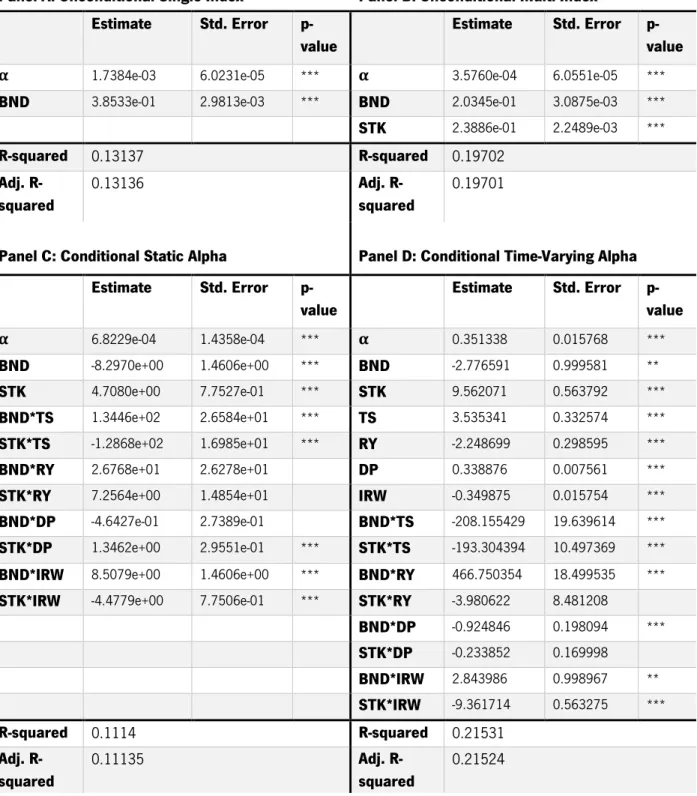
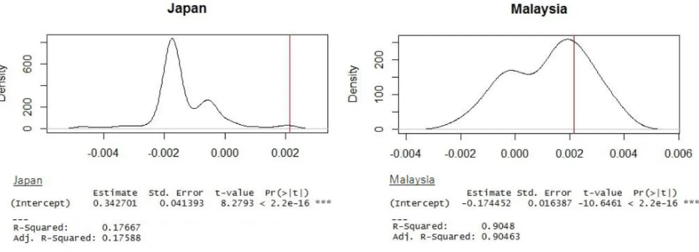
Figure 1 Size of the aggregate local currency bond markets of ASEAN+3. Data provided by the Asian Development Bank. ... 31 Figure 2 Density plot of average fund returns. ... 33 Figure 3 Correlation matrix of the instrument variables. ... 36 Figure 4 Graphical representation of the correlation matrix of the time-series of average returns for the bond samples of each individual country. ... 51 Figure 5 Density plot of average fund returns over the sample period and Alpha estimates for the Japanese and Malaysian bond fund samples estimated using the conditional time-varying alpha model. ... 52

(9)

ix

Table of Tables

Table 1 Summary statistics of the average monthly returns of the bond fund sample. ... 32

Table 2 Summary of public information variables used in the conditional model. ... 35

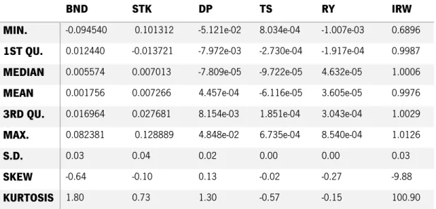
Table 3 Summary statistics of the instrument variables. ... 36

Table 4 Results for the studentized Breush-Pagan and Ljung-Box tests. ... 38

Table 5 Empirical results of the regression for the all-country aggregate fund data using four different models. ... 39

Table 6 Empirical results for the aggregate fund data using the conditional time-varying alpha model after excluding both Japan and Korea from the sample. ... 41

Table 7 Adjusted R-squared values of model specification variants. ... 41

Table 8 Adjusted R-squared values of model specification variants for each individual country. ... 42

Table 9 Bond fund performance results for the Chinese bond fund sample. ... 43

Table 10 Bond fund performance results for the Indian bond fund sample. ... 44

Table 11 Bond fund performance results for the Japanese bond fund sample. ... 45

Table 12 Bond fund performance results for the South Korean bond fund sample. ... 46

Table 13 Bond fund performance results for the Malaysian bond fund sample. ... 47

Table 14 Bond fund performance results for the Thai bond fund sample. ... 48

Table 15 Results for the contingency table analysis of aggregate sample bond fund performance persistence. ... 54

Table 16 Results for the contingency table analysis of Indian bond fund performance persistence. ... 55

Table 17 Results for the contingency table analysis of Chinese bond fund performance persistence. ... 56

Table 18 Results for the contingency table analysis of South Korean bond fund performance persistence. 57 Table 19 Results for the contingency table analysis of Malaysian bond fund performance persistence. ... 58

(10)

1

Chapter 1 - Introduction

A substantial portion of investments is made by professional fund managers, rather than by individual investors. This makes assessing the value provided by these services a subject of great importance to the individual investors who invest in these funds. Bond funds make for an important part of the investment fund market, and so an analysis of their performance is relevant for investors. Additionally, authors such as French and Poterba (1991) have argued that US investors tend to underinvest in foreign markets and thus miss out on diversification opportunities. This apparent under diversification of investors makes studying the performance of foreign bond funds even more important.

Traditional models of fund performance evaluation are designated unconditional in the sense that no information about the state of the economy is used to predict returns. These models assume that expected risk and returns remain static over time. However, in reality, they are time-varying. When fund managers employ dynamic strategies that respond to changes in public information unconditional models will give a biased view of performance as they will entangle the time variation of required risk premiums with abnormal performance (among others, Jensen (1972), Admati and Ross (1985) and Grinblatt and Titman (1989)). Furthermore, models that do not take into account any information about the state of the economy may also lead to erroneous conclusions regarding the persistence of performance. Evidence of persistence of performance using unconditional models may reflect the persistence of the time-variance of expected risk and returns rather than that of fund performance.

Several studies have shown that conditioning information on certain publicly available information variables is useful when predicting stock and bond returns (among others, Keim and Stambaugh (1986), Fama and French (1989) and Ilmanen (1995)) when considering time-varying risk. Conditional performance evaluation models look at fund performance by taking into account changes in public information variables that affect expected risk premiums, which may lead to different conclusions regarding performance and persistence of performance than when no information regarding the state of the economy is taken into account.

(11)

2

More recently, a growing amount of research applies conditional models of performance in the context of bond funds (among others, Silva, Cortez and Armada (2003) and Ayadi and Kryzanowski (2011)). This literature suggests that conditional models of performance offer greater explanatory power than their unconditional counterparts and that unconditional models tend to understate fund performance.

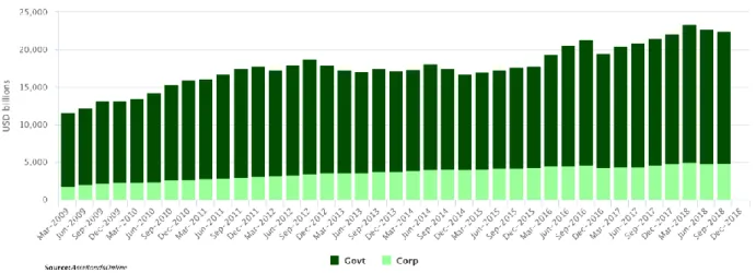
The East Asian bond market has been developing rapidly in the 21st century. Data from the Asian

Development Bank shows the aggregate local-currency bond market size of the aggregate ASEAN+31

countries has roughly doubled over the past decade. Despite rapid developments in both East Asian bond markets and the bond fund performance literature, we found, to the best of our knowledge, no study that applies recent developments in performance evaluation, most preeminently conditional models of performance, to the performance of bond fund managers from East Asian countries.

In this dissertation, we evaluate the performance of East Asian bond funds from 6 different countries: Japan, China, South Korea, India, Malaysia and Thailand. We will examine the performance of bond funds using single and multi-index models in both a conditional and an unconditional form. The main goal of this analysis is to ascertain whether East Asian bond fund managers are able to outperform their benchmark on a risk-adjusted basis and to study the impact of public information variables on explaining fund performance. We also study the persistence of performance of East Asian bond funds.

We follow Ferson and Schadt (1996)’s specification of a conditional model of performance. The alpha obtained from this model serves as measure for the risk-adjusted performance of East Asian bond funds. We also apply Christopherson et al. (1998)’s extended conditional model to capture the time-variance of alpha due to changes in public information variables. The persistence of bond fund performance will be assessed by means of a contingency table analysis.

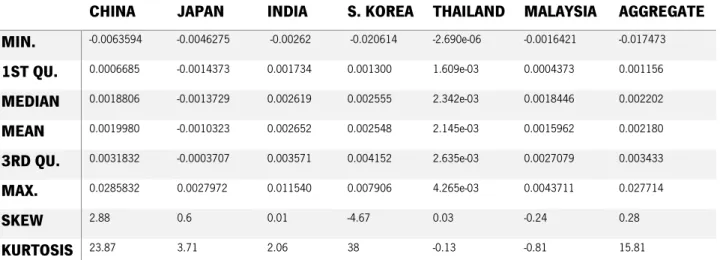
Our sample consists of bond funds from six different East Asian countries: China, India, Japan, South Korea, Thailand and Malaysia. We collect monthly net return data for 395 Korean bond funds, 144 Japanese bond funds, 787 Chinese bond funds, 83 Malaysian bond funds, 1069 Indian bond funds and 44 Thai bond funds, for a total of 2522 East Asian bond funds. Our sampling period starts in January of 2009 and ends in November of 2018.

1_{The ASEAN+3 region consists of the member countries of the Association of Southeast Asian Nations plus China,}

(12)

3

Overall, we find that, on average, East Asian bond funds managers are able to deliver superior risk-adjusted returns, although evidence regarding performance varies at the country level. We also find that the performance of East Asian bond funds is not persistent.

This dissertation is divided into seven chapters. The present chapter introduces and contextualizes the subject matter as well as present an overview of the structure of the dissertation. In the second chapter, we delve into a review of the literature regarding bond fund performance. In the third chapter, we discuss the empirical methodology used in our analyses and, in the fourth chapter, we present the data regarding our sample and instrumental variables, as well as discuss important aspects regarding the computation of variables. We present our empirical results in the fifth chapter. We also discuss those results and address the main concerns, limitations and issues regarding our methodology and the models of performance we use in the fifth chapter. In the sixth and final chapter, we present the main conclusions of this dissertation.

(13)

4

Chapter 2 - Review of the Literature

2.1 - Overview of Bond Fund Performance

Cowles (1933) compared the average return of a set of active portfolios with the return of a passive portfolio and concluded that the active portfolios underperformed the passive portfolio. However, Cowles’ analysis of performance took only fund returns into account. A true assessment of fund performance and managerial skill must also take into account the risk that is taken in order to generate those returns. Modern Portfolio Theory (MPT) introduced by Markowitz (1952) formulates the investor’s portfolio selection problem in terms of both risk (measured by the variance of portfolio returns) and returns. According to Markowitz, investors would optimally hold a mean-variance efficient portfolio, that is, a portfolio with the highest expected return for a given level of risk and the minimum level of risk for a given level of expected return. Tobin (1958) extends MPT by including a risk-free asset, such that the optimal portfolio results from a combination between the risk-free asset and one risky portfolio.

In 1968 Michael Jensen publishes a study of the performance of 115 open-end mutual funds from the period of 1955 to 1964. Jensen’s analysis is centered on the problem of how to infer fund manager skill by the returns they gain after taking in consideration the amount of risk their portfolio entails. Risk-adjusted performance, Jensen argues, should be analyzed through a fund manager’s predictive ability, that it, “the ability to earn returns through successful prediction of security prices which are higher than those which we could expect given the level of riskiness of his portfolio”. He thus evaluates mutual fund performance using the CAPM model in order to capture performance adjusted for the fund’s exposure to market risk. We write the general form of a single-index model of performance as follows.

𝑅_𝑖𝑗 = 𝛼_𝑖 + 𝛽_𝑖𝐼_𝑡+ 𝜖_𝑖𝑡 (1)

where

𝑅𝑖𝑗 = the excess return on the ith fund during time t

𝛼_𝑖 = the average excess risk-adjusted return for the ith fund

(14)

5

𝐼_𝑡 = the excess return of the appropriate benchmark at time t and a residual term 𝜖_𝑖𝑡

In this equation the term 𝛼𝑖, henceforth referred to as Jensen’s Alpha, provides a risk-adjusted

measure of fund performance. By estimating a linear regression of the single-index model for his data on mutual funds, Jensen finds that on average mutual fund managers were not able to beat a passive, buy-and-hold market portfolio, strategy on a risk-adjusted basis.

Rosenberg and Guy (1976) formulate an extension to the aforementioned single-index model in order to allow for multiple sources of systemic risk. The general form of the multi-index model can be written as follows.

𝑅𝑖𝑗 = 𝛼𝑖 + ∑𝐾𝑗=1𝛽𝑖𝑗𝐼𝑡𝑗+ 𝜖𝑖𝑡 (2)

Like the single index model, we can think of the betas as the set of weights on a set of passive portfolio that best replicates the fund’s performance.

The general intuition behind these multi-factor models comes from Arbitrage Pricing Theory (APT) as proposed by Ross (1976). The concept of no arbitrage introduced by APT states that, should the price of a security diverge from what is predicted by systemic risk premiums, arbitrageurs would buy or sell that security so that such a divergence will quickly disappear. If conditions for no arbitrage are met (that is, if we are working within the limits of arbitrage that are described by Shleifer and Vishny (1997)) then the excess return of any given security will converge to the sum of the risk premiums associated with each risk-factor multiplied by their respective betas.

Roll and Ross (1980) perform an empirical evaluation of Arbitrage Pricing Theory using data for individual equities during the 1962–1972 period and find that at least three factors, possibly four, are necessary to explain the return generating process of stocks. Many authors since then have proposed various different specifications of multi-index models in the context of APT controlling for different possible sources of systemic risk.

One example of such a multi-index model is Fama and French’s (1993) three-factor model that adds two factors in addition to the market portfolio, one factor for size and another for book-to-market equity. With this three-factor model, they find that we are able to explain the returns of a sample of stocks more

(15)

6

exactly than the single-factor model that account only for market exposure. Fama and French (1993) build a different model this time with two risk-factors pertaining to the bond market in addition to the three stock market risk-factors. These two bond market risk-factors capture maturity and default risk, respectively. With this five-factor model, Fama and French find they are able to explain the returns of a sample of securities for both the stock and the bond market (except for the particular case of low-grade corporate bonds).

Multiple index models generally have better explanatory power than their single-index counterparts, they also control for multiple risk sources better than single-index models, which generally results in lower alphas than those estimated by single-index models (Ippolito (1989)). Single-index models attributed the excess return that fund managers earned over the market benchmark to superior managerial skill and information. However, this result shows that these returns are instead generated through exposure to hitherto unaccounted for systemic risk-factors. Moreover, measures of performance in both equity and balanced funds have been shown to be highly sensitive to the choice of risk-factors (Lehman and Modest (1987) and Elton and Gruber (1992)). In fact, studies on both equity and balanced funds have found that using multi-index models can affect the rankings of fund performance (among others, Grinblatt and Titman (1989b) and Connor and Korajczyk (1991).

Blake, Elton and Gruber (1993, 1995) are, to the best of our knowledge, the first to study the performance of bond funds specifically using both single and multi-index models of performance. They use two samples, the largest of which suffers from survivorship bias, which the authors argue does not impact bond funds to the same extent it does equity funds since bonds are a less volatile asset and bond funds are therefore less likely to dissolve or merge. They first analyze fund performance using a single-index model, where the fund’s excess returns over a riskless asset are linearly related to the return of a benchmark index, similar to the market model widely used in evaluating the performance of equity portfolios.

Overall, Blake, Elton and Gruber (1993) find that the bond funds in their sample underperformed relevant indexes on a post-expenses basis. Interestingly, their results suggest that performance before expenses is neutral, as the underperformance was approximately equal to the average management fees. Indeed, they find that, on average, a percentage point increase in expenses leads to a percentage point decrease in returns. Lakonishok (1981) and Philpot et al. (1998) also find a significant inverse correlation between a fund’s abnormal return and their expense ratio for a sample of 70 mutual funds and 27 bond

(16)

7

funds, respectively. Gallagher and Jarnecic (2002) echo this conclusion for a sample of Australian bond funds.

Cici and Gibson (2012) argue that inability to employ holdings based measures of performance, like had been done for equity funds, has stopped researchers from being able to dig deeper into active bond fund management. The authors focus on the question of whether fund managers capitalize on firm-specific research in order to select bonds that outperform similar issues. They argue that the question of fund manager selectivity pre-expenses is important even if post-expense performance is negative, as a manager with security selection skills may be hampered by structural handicaps (Wermers (2006)), for example, volatile net investor flows may force costly bond trading, reducing net returns. The results they obtain suggest that, on average, fund managers are not able to pick corporate bond funds that outperform relevant benchmarks, for both high-yield and investment-grade corporate bonds. Furthermore, they examine the aggregate holdings of all funds in particular bonds to proxy for fund managers’ collective valuation assessments and found that high-yield bonds with low collective ownership outperformed issues with high collective ownership (for investment-grade bonds they find no difference in performance between high and low ownership bonds). The authors argue that this result raises the question of whether bond mutual funds as a group are either at an informational or liquidity disadvantage relative to other categories of institutional investors in fixed-income markets, for example, they point out that the counterparties with which bond funds trade in the corporate bond market (such as life insurance companies, which are the largest holder of corporate bonds in the U.S. market) rarely engage in liquidity trading. On average, they find that the combined effect of security selection and characteristic timing added 27 and 4 basis point per year to the performance of investment-grade and high-yield bond funds, respectively. In contrast, they estimate that management fees and transaction costs for investment-grade and high-yield bond funds for their sample period totaled 88 and 138 basis points per year, showing that the costs of active management far outweighed the benefits.

(17)

8

2.2 - Conditional Models of Performance

The models of performance that have been presented so far have been unconditional models. We now turn our attention towards conditional performance models. Unconditional measures of performance, that is, measures in which no information about the future state of the economy are used, such as Jensen’s alpha that was discussed previously, have been shown to be biased when managers follow dynamic strategies due to time-varying risk (among others, Jensen (1972), Dybvig and Ross (1985a)). Unconditional models of performance ascribe such dynamic strategies to managers possessing superior information about the market, which translate itself in market timing ability.

Treynor and Mazuy (1966) use convexity in the relation between the fund’s return and the benchmark return to identify market timing ability. We can extend equation (1) to include this measure of market timing as shown in the equation below.

𝑅𝑖𝑡 = 𝛼𝑖 + 𝛽𝑖𝐼𝑡+ 𝛬𝑖𝐼𝑡2+ 𝜖𝑖𝑡 (3)

A positive value for 𝛬_𝑖 indicates market timing ability, as when the market is up (down) a fund able to time the market will be up (down) by a greater (lesser) amount than what the market model would predict.

Merton (1981) and Henriksson and Merton (1981) measure market timing ability by the excess return obtained by the manager that cannot be replicated by a mix of call options and the market portfolio.

(𝑅𝑖𝑡− 𝑟𝑓𝑡) = 𝛼𝑖 + 𝛽1,𝑖(𝐼𝑡− 𝑟𝑓𝑡) + 𝛽2,𝑖(𝐼𝑡− 𝑟𝑓𝑡)𝐷 + 𝜖𝑖𝑡 (4)

Where 𝑟_𝑓 is the risk-free rate at time t and D is a dummy variable that is equal to 1 when 𝐼_𝑡> 𝑟_𝑓𝑡 and 0 otherwise (note that so far in our notation we have used 𝑅_𝑖𝑡 and 𝐼_𝑡 as the excess returns for both the portfolio and the index, respectively, over the risk-free rate, while here they denote the absolute returns). The intuition here is that we consider a time when 𝐼𝑡> 𝑟𝑓𝑡 to be a bull market and a bear market when the

reverse is true, which means that a manager with market timing ability would balance their portfolio such that it’s beta is equal to 𝛽_1,𝑖 in a bear market and 𝛽_1,𝑖+ 𝛽_2,𝑖 in a bull market, therefore a statistically significant 𝛽_2,𝑖 indicates market timing ability.

(18)

9

Cici and Gibson (2012) adapt a model previously applied to market timing in equity funds by Wermers (2000). 𝐶𝑇𝑡 = ∑ (𝜔𝑏,𝑡−1𝑅𝑡 𝑃𝑏,𝑡−1 − 𝜔𝑏,𝑡−5𝑅𝑡 𝑃𝑏,𝑡−5 𝑁 𝑏=1 ) (5)

The characteristic timing (CT) measure subtracts the quarter t return of the quarter t −5 matching characteristic portfolio for bond b (times the portfolio weight at the end of quarter t −5) from the quarter t return of the quarter t −1 matching characteristic portfolio for bond b (times the portfolio weight at the end of quarter t −1), thus capturing the contribution to holdings returns from changes in portfolio characteristic weights that occurred over the prior year. If a manager successfully rebalances portfolio weights towards those characteristics that subsequently exhibit high payoffs the CT measure will be positive, indicating market timing ability. Using this method they find no timing ability for a sample of investment-grade corporate bond funds, but find that managers of high-yield corporate bond funds, on average, show market timing ability.

Treynor and Mazuy (1966)’s model relies on convexity in the relation between the fund’s returns and the common factors, however this convexity (or concavity) can arise for reasons unrelated to the manager’s market timing ability, so Chen, Ferson and Peters (2010) argue that it’s important to control three potential biases of non-linearity unrelated to market timing ability: non-linear relation between market factors and a fund’s underlying asset, this non-linearity is likely to exist in bond funds, since bond returns are non-linearly related to interest rate changes and callable and convertible bonds contain explicit option components, so a portfolio containing these last two assets will bear a convex relation to the underlying asset (Jagannathan and Korajczyk (1994)); interim trading, meaning the fund rebalances more frequently than the return observation interval; stale pricing, arising from thin or nonsynchronous trading (which has been shown to introduce a downward bias in the estimates of a portfolio’s beta by Fisher (1966) and Scholes and Williams (1977); and availability of public information that affects future asset returns. They find that the impact of nonlinearities on inferences on market timing ability is significant as without controlling for non-timing related non-linearity fund managers would appear to have negative market timing ability, after controlling for these biases the market timing ability of the funds becomes neutral to slightly positive.

(19)

10

Conditional models of performance propose a different interpretation. If we allow for time variance of risk premia then the unconditional alpha defined as the past average excess return of the fund over the average market excess return no longer states fund performance on a risk-adjusted basis. Ferson and Schadt (1996) thus propose the following interpretation of conditional models of performance: that if the dynamic strategies employed by an actively managed portfolio can be replicated by using only publicly available information then that fund should not be judged as presenting superior performance.

This framework interprets market timing in a manner similar to the market timing model of Merton (1981), in the sense that active fund managers respond dynamically to information regarding the state of the economy, from the point of view of conditional models, however, they do not do so due to possessing superior information but rather due to publicly available information regarding certain variables that are found to be predictive of future market returns.

A conditional performance measure has been defined as “a measure of performance of a managed portfolio taking into account the information that was available to investors at the time” (Farnsworth, 1997, p.23), which reflects the fact that managers take into account changes in certain public information variables and adjust their portfolios accordingly. Keim and Stambaugh (1986) and Fama and French (1989) have shown that these public information variables are important in explaining the returns of both stocks and bonds. Ferson and Schadt (1996) apply this concept to portfolio performance evaluation by extending equation (1) in order to include public information variables by making beta a linear function of a vector of predetermined information variables 𝑍_𝑡−1 that are empirically shown to be predictive of asset returns such that

𝛽_𝑖(𝑍𝑡−1) = 𝛽0𝑖+ 𝛽𝑖′𝑧𝑡−1 (6)

Where 𝛽_0𝑖 is the unconditional beta and 𝑧_𝑡−1= 𝑍_𝑡−1− 𝐸(𝑍) is the vector of deviations of 𝑍_𝑡−1 from the average vector. Applying this to equation (1) we get

𝑅𝑖𝑗 = 𝛼𝑡+ 𝛽0𝑖𝐼𝑡+ 𝛽𝑖′(𝑧𝑡−1𝐼𝑡) + 𝜖𝑖𝑡 (7)

Christopherson et al. (1998) further extend this model in order to allow alpha to vary with the information variables such that

(20)

11

Including the conditional alpha in equation (7) we get

𝑅𝑖𝑗 = 𝛼0𝑖+ 𝐴𝑖′𝑧𝑡−1+ 𝛽0𝑖𝐼𝑡+ 𝛽𝑖′(𝑧𝑡−1𝐼𝑡) + 𝜖𝑖𝑡 (9)

We can easily adapt this model to a multi-index framework by including the cross products of each factor with the information variables, we thus get the general form of the conditional multi-index model of performance.

𝑅_𝑖𝑗 = 𝛼_0𝑖+ 𝐴_𝑖′𝑧_𝑡−1+ ∑_𝑗=1𝐾 𝛽_𝑖𝑗𝐼_𝑡𝑗+ ∑𝐾_𝑗=1𝛽_𝑖𝑗(𝑧_𝑡−1𝐼_𝑡𝑗) + 𝜖_𝑖𝑡 (10)

The necessity of this extension to the model to allow for time-varying alphas is rooted in the fact that active fund managers often employ more information than is publicly available when constructing a set of portfolio weights. Christopherson at al. (1998) argues that, if the set of portfolio weights held by the manager carry no more information about future returns than the set of public information variables 𝑍_𝑡−1, then the conditional alpha will be zero, that is, the total alpha will be equal to the unconditional alpha as in equation (4). However, if active strategies employed by the fund manager use more information than is contained in 𝑍_𝑡−1 the set of portfolio weights will be conditionally correlated with future returns. This means that the conditional alpha is a is function of the conditional covariance between the set of portfolio weights and future returns, given 𝑍_𝑡−1, and therefore the total alpha is also a function of 𝑍_𝑡−1.

Ferson and Schadt (1996), Hansen and Jagannathan (1991) and Cochrane (1992) note that the regression of the conditional model can be interpreted as an unconditional multifactor model where the products between the risk factors and the lagged information variables represent additional factors, therefore the conditional alpha is the excess return over the average return of the dynamic strategies replicated by those factors. Finally, as Ferson and Schadt (1996) also note, conditional models raise important questions about optimal investment decisions, in a dynamic strategy framework the investment horizon of the investor becomes a more complex issue and the form of the model is no longer invariant to the return measurement interval

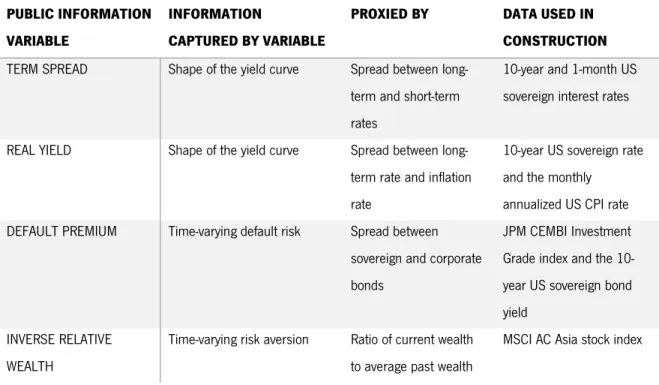
As we previously mentioned, the public information variables that make up the vector 𝑍𝑡−1 are

chosen because of their predictive ability of future asset returns. There are numerous studies that examine empirically the ability of certain variables in predicting bond returns. Mankiw (1986), Bisignano (1987) and Solnik (1993) find evidence that the term spread, that is, the spread between a long-term bond and a

(21)

short-12

term bond, are predictive of government bond returns. The motivation behind this instrument is to proxy for overall time-varying expected bond risk premium by reflecting the shape of the yield curve (Fama and Bliss (1987) and Campbell and Ammer (1993)). Research using this instrument in conditional models of performance include Ilmanen (1995), Silva et al. (2003), Fama and French (1989), Deaves (1997), Gebhardt et al. (2005) and Ayadi et al. (2011). Another proxy for time-varying risk through the shape of the yield curve is the real bond yield, which is the spread between a long term bond and the average inflation rate over the remaining life of that bond.

Campbell and Ammer (1993) explain in more detail how the term spread and real bond yield represent the shape of the yield curve and thus capture overall bond time-varying risk premia. They show that the continuously compounded yield 𝑦_𝑛,𝑡 of an n-period nominal discount bond per period is:

𝑦_𝑛,𝑡 = (1

𝑛) 𝐸𝑡∑ (𝜋𝑡+1+𝑖+ 𝜇𝑡+1+𝑖+ 𝑥𝑛−1,𝑡+1+𝑖) 𝑛−1

𝑖=0 (11)

Where π is the n-period average of expected inflation rates, µ the n-period average of expected real rates of a one-period nominal bond and 𝑥 is the n-period average of expected bond risk premia. This equation shows that the bond yield contains information about future expected bond risk premia. The bond yield is then a noisy proxy for expectations of the right hand side terms. Nevertheless, we can construct less noisy instruments by subtracting from the bond yield other variables that reflect expected future risk. We can write the general form of the per-period term spread and real bond yield, respectively, as follows:

𝑇𝑆_𝑛,𝑡 = 𝑦_𝑛,𝑡− 𝑦_1,𝑡=(1 𝑛) 𝐸𝑡∑ [(𝑛 − 1 − 𝑖)(Δ𝑦1,𝑡+2+𝑖) + 𝑥𝑛−𝑖,𝑡+1+𝑖 𝑛−1 𝑖=0 (12) 𝑅𝑌_𝑛,𝑡 = 𝑦_𝑛,𝑡− (1 𝑛) 𝐸𝑡∑ 𝜋𝑡+1+𝑖 𝑛−1 𝑖=0 = ( 1 𝑛) 𝐸𝑡∑ (𝜋𝑡+1+𝑖𝜇𝑡+1+𝑖+ 𝑥𝑛−1,𝑡+1+𝑖) 𝑛−1 𝑖=0 (13)

Ilmanen (1995) argues that the set of chosen information variables must capture time-varying risk aversion in addition to time-varying risk, in order to accomplish this he suggests an additional variable: the inverse relative wealth. They propose that relative risk aversion is inversely proportional to relative wealth. To clarify this we will consider Marcus (1989)’s wealth-dependent model of utility.

(22)

13

𝑈(𝑊) =(𝑊−𝜔)1−𝛾

1−𝛾

(14) Where W signifies wealth, 𝜔 is the minimum subsistence level of wealth and γ is a positive constant. Rational agents never let their wealth fall below subsistence level as they will suffer infinite disutility when 𝑊 = 𝜔 and so the agent will become increasingly risk-averse as wealth decreases toward the subsistence level. We therefore write relative risk aversion (RRA) as

𝑅𝑅𝐴 = −𝑊𝑈𝑤

𝑈𝑤 =

𝛾

1−_𝑊𝜔 (15)

And define the inverse relative wealth as

𝐼𝑅𝑊_𝑡= 𝑒𝑤𝑎[𝑊𝑡−1]

𝑊𝑡

(16) Where 𝑒𝑤𝑎[𝑊_𝑡−1] is the exponentially weighted average of past wealth, here the author is chooses a smoothing coefficient of 0.9 in order to make the last 36 months of observations make up 95% of the cumulative weight of the weighted average and thus capture business cycle effects. Ilmanen (1995) uses a stock market index as proxy for aggregate wealth arguing that, despite being only a small part of aggregate wealth (Ibbotson, Siegel and Love (1986)), stock markets represent the most volatile segment of wealth and are correlated with other parts of wealth.

If we consider an investable universe not limited only to default-free bonds we must also consider a proxy for time-varying default risk. Gebhardt et a. (2005) study the cross-section of corporate bond returns using a two--factor model that includes the term spread and introduces a term for default risk. In order to proxy for overall default risk the default risk premium is constructed as the spread between an index of investment grade corporate bonds and long-term sovereign bonds. They find that the corresponding betas of these two instruments perform better in forecasting bond returns than characteristics such as duration and rating, they also find, however, that those characteristics contain information about the systemic risk borne by the term spread and default premium of a corporate bond. Fama and French (1989) also study corporate bond returns using the same two instruments and, in addition to the findings already mentioned, find that the default premium is correlated with the stock market dividend yield and long-term business conditions. Ilmanen (1995), Deaves (1997), Yamada (1999) and Silva (2004) also study the impact of public information variables in various bond markets and find them to have predictive ability for bond

(23)

14

returns. However, it should be noted that in most cases conditional models only explain a relatively small part of the variance of bond returns.

This model was initially applied only to stock funds or pension funds (Chen and Knez (1996), Dahlquist and Söderlind (1999), Otten and Bams (2002), Grünbichler and Pleschiutsnig (1999)), for both the US and European markets, and the evidence suggests that unconditional models tend to understate performance and that conditional models also add explanatory power.

Silva et al. (2003) is, to the best of our knowledge, the first study to apply conditional models of performance in the context of bond funds. The authors argue that conditioning information in evaluating bond fund performance is more critical than in stock funds, as bond fund managers tend to be market timers more so than security pickers, and therefore unconditional measures of performance may not be appropriate primarily due to their underlying assumption of constant risk, more specifically, if a bond fund manager correctly anticipates a change in a relevant economic variable such as, for example, an increase (decrease) in interest rates they should decrease (increase) their portfolio’s duration, since duration is closely related to beta the unconditional (static) beta from equation (1) becomes a biased measure of performance.

Silva et al. (2003) analyze the performance of a sample of European bond funds from six different countries. The sample consists of 58 funds from Italy, 266 funds from France, 90 funds from Germany, 157 funds from Spain, 45 funds from the UK and 22 funds from Portugal, for a total of 638 European bond funds whose monthly return data is gathered for the period of February of 1994 to December of 2000 (except in the case of the Portuguese bond funds, for whom the return data is only available from January of 1995 onwards). Performance is evaluated using Christopherson et al.’s (1998) time-varying alpha conditional model in both a single and multi-index configuration. For the single-index model, Silva et al. (2003) use the SalomonSmithBarney WGBI all maturities for each country as a bond market benchmark. For the multi-index model, they add a stock market factor and the default premium. As a benchmark for the stock market they use the MSCI stock index for each individual country in the sample, for the default spread, however, they opt to use an aggregate spread for the Eurozone, calculated as the difference between the MSCI Euro Credit Index BBB rated and the MSCI Euro Credit Index AAA rated, as the corporate bond market for most individual European countries was still fairly illiquid at the time of their analysis. For the

(24)

15

conditional versions of these single-factor and three-factor models they add three predetermined information variables: the term spread, the real bond yield and the inverse relative wealth.

Four main conclusions can be drawn from Silva et al’s (2003) analysis. First, bond funds underperformed the benchmark in all scenarios (for both conditional/unconditional and single/multi-index models). Second, they confirm the already mentioned conclusion of Ippolito (1989) that including additional risk-factors in the model provides greater explanatory power and that single-index models tend to overstate risk-adjusted performance. Third, consistent with what was found for equity funds, incorporating predetermined information variables generally causes bond funds to exhibit slightly better performance, although, for some countries, using conditional models seems to decrease alpha (it is worth noting that, despite most studies finding that conditional models improve performance, Chen and Knez (1996) argue that the directional change in performance results due to conditioning information can be in either direction and is likely to be sample and period specific). Fourth, the results show that conditional models have more explanatory power than their unconditional counterparts, however, they also find that the impact of additional risk-factors is greater than the impact of incorporating predetermined information variables.

Ayadi and Kryzanowski (2011) analyze the performance of 303 Canadian bond funds (209 of which are still active at the end of the sample period and 94 that are not) over the period of January of 1984 to the end of December of 2003. In their analysis, they employ a conditional model that uses five information variables: the term spread, the default premium, the inverse relative wealth, the lagged risk-free rate and the real bond yield. They also test the model using both net and gross return, in order to ascertain the impact of management fees on fund performance. They report that their sample of bond funds presents a positive alpha using gross returns and negative for net returns. This is consistent with the findings of Blake, Elton and Gruber (1993) in what has proven to be one of the most persistent results in the fixed income fund literature, that bond fund underperformance is largely driven by management fees. They also find that under conditional models the estimated performance is slightly more positive than under their unconditional counterparts.

Ghysels (1998) claims that conditional models may produce larger pricing errors than unconditional models due to the assumption of linearity in the time-variance of betas. On the other hand, Farnsworth, Ferson, Jackson and Todd (2002) find that linear time-varying betas produce smaller pricing

(25)

16

errors. Silva (2004) says that whether imposing linearity on time-varying betas is helpful or not is not yet a settled matter.

2.3 - Persistence of Performance in Bond Funds

The study of the persistence of performance is of equal importance to the subject of fund performance as the assessment of performance itself is. If past performance is not a predictor future performance then the matter of evaluating fund performance becomes irrelevant to investors. Persistence of performance means that a fund with good (poor) performance in a given period is likely to also be a good (poor) performer in the future. Evidence of persistence of performance would signify a violation of the efficient market hypotheses (as in an efficient market performance is assumed to be randomly distributed through time) and it would also mean that investors could realize abnormal gains by buying recently well-performing funds and selling poor well-performing ones or vice-versa, if there is evidence that performance tends to reverse, that is, that good (poor) performing funds in a given period are likely to show poor (good) performance in the next.

In equity funds, the evidence for the persistence of fund performance is mixed, the case for bond funds is no different in this regard, although the evidence for bond funds presents less indication of persistence of performance than in equity funds.

Blake, Elton and Gruber (1993) and Philpot et al. (1998) find no evidence of persistence for their sample of bond funds (Blake, Elton and Gruber find evidence of forecasting ability when using a larger sample however it cannot be discarded that this evidence of persistence was due to the presence of survivorship-bias in the sample). Kritzman (1983) confirms this result for a sample of bond funds over the periods of 1972 to 1981. For the German market, Maag and Zimmerman (2000) also find no evidence of persistence in German bond funds, Dahlquist, Engström and Söderlind (2000) reach a similar conclusion for Swedish bond funds. On the other hand, Polwitoon and Tawatnuntachai (2006, 2008) find evidence of short-term persistence for both U.S based global and emerging market bond funds. Khan and Rudd (1995) also find evidence of persistence in bond fund performance for the period of 1986 to 1993.

(26)

17

There are multiple possible methods through which researchers can assess the persistence of performance in bond funds, however, the literature regarding this subject centers around the following three methods: cross-sectional regression of future performance on past performance; measuring the Spearman rank correlation coefficient between future and past performance of bond funds; and contingency tables.

The first of these method consists of estimating the performance of each bond fund in a sample over a set, non-overlapping, evaluation period. This estimate of performance can simply be the Jensen’s alpha obtained by regressing the fund’s excess returns on each evaluation period over relevant risk-factors. As an alternative to alpha, the Shape ratio can be used as a risk-adjusted measure of performance instead. Using a non-parametric measure of performance such as the Sharpe ratio helps avoid spurious results due to a misspecified model of performance. We can then use a standard OLS method to regress the time-series of future performance on past performance and test the significance of the slope coefficient.

The Spearman rank correlation coefficient method works similarly to the first. First, we once again group the fund return data into a chosen evaluation period and estimate performance using a chosen risk-adjusted measure of performance. Next, funds are ranked based on this measure for each time period, we can then calculate the Spearman rank correlation coefficient between the fund ranking of the previous period and that of the subsequent period.

𝜌𝑡,𝑡−1 = 1 −

6 ∑ 𝑑_{𝑡,𝑡−1}2 𝑁(𝑁2₋₁₎

(17)

Where ∑ 𝑑_{𝑡,𝑡−1}2 _{is the sum of the squared differences between the funds’ ranks over the evaluation}

and post-evaluation period, and 𝑁 is the number of ranks. Finally, we estimate, and test the significance of, the slope coefficient of the time-series of correlation coefficients using a standard OLS method.

The contingency tables method consists of assigning funds to one of four cell in a two-by-two contingency table. Each cell represents a certain state of fund ranking based on the relationship between their performance over the past evaluation period and the subsequent period. Funds are labeled either past winners/future winners, past winners/future losers, past losers/future winners and past losers/future losers. A fund is considered a winner if its risk-adjusted performance over the evaluation period ranks above the mean performance over the same period, and is considered a loser otherwise. If there is no relation between past and future performance, that is, if performance is not persistent, each of these four cells

(27)

18

would have an equal frequency of 25%. Finally, the significance of performance persistence is evaluated by performing a Chi-square test on these frequencies.

Huij and Derwall (2008) study persistence of performance for the entire population of U.S. bond funds over the 1990-2003 period using a multi-index, unconditional, model and all three previously mentioned measures of persistence and find strong evidence of persistence. Furthermore, they find that the evidence regarding persistence is not conditional on the chosen method. Silva, Cortez and Armada (2005) study the persistence of the performance of European bond funds using both cross-sectional regression analysis and contingency tables to detect persistence. They obtain evidence that indicates existence of performance persistence whatever the methodology used (additionally, they find that performance persistence is stronger among the poorer performing funds). However, they find that the evidence for persistence is weaker when conditional models are used, suggesting that at least part of the persistence phenomenon is caused by time-varying betas.

Gutierrez, Maxwell and Xu (2009) argue that their finding that bond funds do not exhibit diseconomies of scale has implications for the persistence of performance of bond funds, as Berk and Green (2004) show that continued performance of a mutual fund should not persist in a competitive market as a consistently good performing fund would receive investor inflows that would eventually trigger diseconomies of scale and offset managerial skill (assuming that, for bond flows, diseconomies of scale would eventually exist at some threshold of size). However, Goldstein, Jiang and Ng (2016) show that, for corporate bond funds, the shape of the flow-to-performance curve is concave, contrary to the convex shape usually observed in equity funds. Moreover, they find that this phenomenon is dependent on both market liquidity conditions and the liquidity of the bond in question (when they analyze the more liquid treasury bond funds they find a convex flow-to-performance curve), this is consistent with Chen, Goldstein, and Jiang (2010)’s findings equity funds with more illiquid assets are more prone to investor outflows when performance is poor than funds holding more liquid assets. This means that investors of bond funds that hold illiquid assets and are performing poorly face a first-mover advantage to redeem their cash as they are susceptible to negative externalities due to a wave of redemptions triggered by the poor performance forcing the fund to sell assets in order to meet redemptions.

(28)

19

2.4 - Additional Topics in Bond Fund Performance

2.4.1 – Bond Fund Performance and Turnover Activity

Under no-arbitrage assumptions, bond fund managers should not be able to increase net returns through trading activity. Furthermore, the underperformance of a bond fund engaging in trading activity relative to relevant benchmarks should be, ceteris paribus, equal to the transaction costs incurred by trading activity. Friend et al. (1962) confirm this in their analysis of fund performance, finding a negative inverse relationship between performance and turnover rate for a given portfolio. Philpot et al. (1998) reach similar conclusions regarding the effect of trading activity on bond fund returns and argue that this result should have been expected by conventional wisdom. Bonds, they argue, are relatively homogenous assets, and therefore bond fund managers have little opportunity to obtain abnormal returns through active management compared to their equity fund counterparts. Ippolito (1989), on the other hand, finds no relation between fund returns and turnover. Grinblatt and Titman (1989) obtain a different result, they find that for the specific case of aggressive growth mutual funds the funds with higher turnover activity generated, on average, superior returns. Moneta (2015) finds that, for a sample of almost 1000 US bond funds for the period 1997–2006, bond fund managers generated a positive gross return through trading activity. This added return averaged at 1%, which is approximately equal to the average management fee charged by US bond mutual funds, making average net performance neutral.

The results obtained in the literature regarding turnover activity are unfavorable towards active management. They show that trading activity in bond funds has either failed to create value for investors or that the value created by it is erased by management fees.

2.4.2 - Economies of Scale in Bond Funds

Fund managers, in both the equity and fixed-income market, face a strong incentive to increase the net asset value under their fund’s oversight, as a part of their compensation is, in most cases, determined by a percentage of the net asset value of the assets they manage. Due to this incentive structure bond

(29)

20

funds have a natural tendency to grow, which begets the question: does size impact fund performance? Carter (1950) postulates that large funds should, on average, be able to outperform small funds. He argues that funds can realize economies of scale by having access to more research resources, lower brokerage rates and greater influence on capital markets. More recent evidence, as found by, among others, Grinblatt and Titman (1998), points in a different direction. They find that smaller, more aggressive, funds that focus on high growth assets outperform larger funds. They argue that smaller funds enjoy greater market mobility and are thus able to take positions in small-capitalization issues that their larger counterparts cannot. Gorman (1991) and Chen, Hong, Huang, and Kubik (2004) also find a significant inverse relation between a fund’s net asset value and its risk-adjusted performance.

Philpot et al. (1998) argue that bond funds might differ from their equity counterparts in this aspect. The reason for bond funds having the opportunity to realize economies of scale while equity funds cannot, they argue, is precisely the same reason by which they previously argued that bond fund managers would be unable to add value through trading activity. They postulate that, since bonds are relatively homogenous assets when compared to stocks and different bond issues are closer substitutes for each other than stocks are, large bond funds might not be as hampered in taking large market positions as large equity funds are, therefore large bond funds may be able to realize economies of scale. In addition to this, Edwards, Harris, and Piwowar (2007) find that the average roundtrip cost of executing a $1 million trade in the corporate bond market is 8 basis points higher than the cost to execute a $2 million trade, this is contrary to what happens in the stock market, where trading costs increase with trade order size.

Philpot et al. (1998) analyze a sample of 27 U.S. bond funds over the period of 1982 to 1993, they limit their sample of bond funds to those that invest solely in investment grade bonds. In this sample, they find a significant positive relation between fund size and realized returns. Polwitoon and Tawatnuntachai (2006) also find a positive relation between fund size and performance for a sample of U.S. based global bond funds. The same authors, in a later (2008) study, reach a similar conclusion in their study of emerging market bond funds finding that large funds outperform smaller funds but only on a basis of total returns, finding that this positive relationship between fund performance and size vanishes when considering a risk-adjusted measure of performance such as the Sharpe ratio. Gutierrez, Maxwell and Xu (2009), on the other hand, find no relation between a fund’s performance and total net assets for a sample of U.S. bond mutual funds from 1990 to 2004.

(30)

21

An overview of the literature, therefore, suggests that despite there not being definitive evidence for the existence of economies of scale in bond funds there is also no indication of dis-economies of scale, unlike what was found for equity funds.

2.4.3 - Emerging Market Bond Funds

Authors such as Erb and Harvey (1999) and Viskanta (2000) argue that investment in the bond markets of emerging market countries is impractical due to high idiosyncratic risk and high correlation with other assets classes (studies which were in no small part motivated by the numerous crises that emerging markets suffered during the 90’s such as the 1997 Asian Crisis, the 1998 Russian Crisis, the Brazilian Crisis of 1999 and the Argentina Crisis of 2000). Despite this, emerging market bonds have been a subject of growing importance since improvements in credit ratings and economic conditions of these countries have renewed the interest of high-yield bond investors in these markets. In fact, the IMF reported that between 1995 and 2005 the amount outstanding of emerging market bonds doubled in size every five years, growing from $1 trillion to $4.5 trillion in that time span.

Polwitoon and Tawatnuntachai (2008) analyze a sample of 50 U.S. based bond mutual funds that invest primarily in emerging markets, they then compare the performance of the funds in that sample to that of a sample of 382 U.S. bond funds that invest domestically and a sample of 146 U.S. global bond funds, that is, bond funds that invest both domestically and internationally. Goetzman and Jorion (1999) argue that evaluating the performance of emerging capital markets is difficult and unreliable due to high variance in the return characteristics of assets between different countries and highly volatile market conditions which may not be adequately covered by a brief evaluation period, Polwitoon and Tawatnuntachai, therefore, use the period of 1996-2005 which, they argue, covers the full cycle of emerging market conditions including the previously mentioned crises and the following rallies. Using the Sharpe ratio as a measure of risk-adjusted performance they find that all three categories of bond funds underperformed their benchmark, however, they also find that the emerging market bond funds outperformed both the domestic and global bond funds.

(31)

22

Polwitoon and Tawatnuntachai (2008) also study the diversification benefits of emerging market bond funds, for this analysis they use Elton, Gruber and Rentzler’s (1987) method which states that a gain in diversification occurs when a new asset is added to an existing asset if the Sharpe ratio of the new asset (𝑆𝐻𝑅_𝑛𝑒𝑤) is greater than the product of the Sharpe ratio of the existing asset and the correlation between the new and existing assets (𝑆𝐻𝑅_𝑎𝜌_{𝑛𝑒𝑤,𝑎}), that is, a new asset provides incremental diversification benefits to an existing asset if the reward-to-risk ratio between the new and existing assets is greater than one (Polwitoon and Tawatnuntachai (2006)). The authors find that, during their sample period, adding 20% of emerging market bond funds into existing portfolios adds an increase of 0.9% to 1.5% in average returns per year without increasing risk, for all existing assets. In a previous study, they had found similar results for U.S. global bond funds, suggesting that U.S. investors specializing in domestic bond funds can enhance return by 0.5–1% per year without increasing risk by incorporating global bond funds in their portfolios (Polwitoon and Tawatnuntachai (2006)).

Emerging market bond funds are therefore an increasingly important subject as they provide a relatively inexpensive and convenient way for investors to get diversified exposure to emerging country bond markets.

2.4.4 - Socially Responsible Investing and Bond Funds

Socially responsible investment (SRI) bond funds are a rapidly growing sector of the financial market and have therefore received considerable attention from academic researchers in recent years. A corporation’s social responsibility (CSR) status is assessed by means of a weighted average score based on their policies regarding various Environmental, Social and Governance (ESG) issues. Therefore, the rise in wealth invested in socially responsible investment products has been accompanied by an increase in ESG rating providers.

Kempf and Oshtoff (2007) study the performance of SRI products by constructing a portfolio that takes long positions in stocks belonging to companies with high ESG rating and is short stock with low ESG ratings. The result of this experiment was an abnormal return of 8.7% relative to the relevant benchmark for a sample of US stocks over the period 1991-2004. Likewise, Derwal et al. (2005) show that, over the

(32)

23

period of 1995-2003, a portfolio composed by companies with high environmental ratings outperformed the benchmark by 4.15% and, furthermore, outperformance a portfolio of companies with a low rating by 6%.

These hypothetical portfolios, however, do not answer the question of whether SRI equity funds actually outperform the market benchmark and their conventional counterparts. Bauer et al. (2005, 2007) and Renneboog et al. (2008a,2008b), among others, analyze the performance of SRI equity funds and generally there does not seem to be any significant difference in performance between SRI equity funds and non-SRI funds.

Bonds are generally less susceptible to idiosyncratic risk than stocks, as the literature shows that bond returns are mostly determined by a small number of non-diversifiable risk-factors. However, Derwall and Koedijk (2009) argue that some types of bonds, such as high-yield bonds, have a significant portion of idiosyncratic risk that can be diversified away by employing active portfolio strategies. It is in this context of diversification benefits that SRI is of most interest for bond funds.

Henke (2016) analyses the performance of 103 U.S. and Eurozone socially responsible bond funds compared to an equal sample of conventional bond funds over the period of 2001 and 2014 using Elton et al’s (1995) five-factor model and found that, over the sample period, the socially responsible funds outperformed their conventional counterparts by 0.5% per year, on average. Furthermore, they conduct a holdings-level analysis that reveals that this source of outperformance can be attributed to the exclusion of corporate bond issued by companies with poor ESG scores.

Goldreyer and Diltz (1999) evaluate the performance of U.S. SRI funds for the 1981-1997 period using an unconditional single-index model and find that the average Jensen’s alpha for the SRI funds is negative while conventional funds achieved positive alphas. Derwall and Koedijk (2009) analyze bond and balanced SRI funds over the 1987-2003 period using an unconditional multi-factor model and found that SRI bond funds showed similar performance to that of characteristics-matched conventional portfolios, while the balanced funds in their sample showed superior performance to their conventional counterparts.

So far we have only discussed SRI strategies that involve negative (positive) screen for companies with low (high) ESG scores, but ESG risk is also present in sovereign bonds. For example, in sovereign bonds, the credit risk is connected not only to political and economic factors but also to social and

(33)

24

sustainability factors (Cantor & Packer (1996) and Mellios & Paget-Blanc (2006)). Factors that, as Derwall and Koedijk (2009) argue, can be mitigated by incorporating ethical and social criteria in portfolio management. Hoepner et al. (2016), for instance, show that countries with higher ESG scores regarding sustainability factors face a lower cost of debt. Drut (2010) also find that a portfolio comprised only of socially responsible government bonds can be constructed such that the investor does not lose any potential for diversification, that is, a bond portfolio that selects government bonds based on a SRI screen is not compromised in terms of mean-variance efficiency.

Leite and Cortez (2018) evaluate the performance of a sample of European SRI bond and balanced funds over the 2002-2014 period using a conditional multi-index model and find that, while the average performance of both SRI and conventional funds was negative, SRI bond funds significantly outperformed their conventional counterparts. They also find that SRI and conventional balanced funds showed similar performance, suggesting that gains from SRI screening are more likely to originate from bond rather than equity holdings. Furthermore, they find that the main ESG risk-factor for SRI bond funds originates from the sovereign, rather than the corporate, bond market, in the form of country-specific risk. Unlike Henke (2016) who, as we mentioned before, found that the superior performance of SRI bond funds was based on the exclusion of corporate bonds from companies with poor CSR practices. Derwall and Koedijk (2009), on the other hand, find that SRI bond funds exhibited similar performance to their conventional counterparts over the period of 1987-2003 while SRI balanced funds outperformed conventional balanced funds over the same period.

(34)

25

Chapter 3 - Methodology

3.1 - Bond Fund Performance

The purpose of this study is to ascertain whether East Asian bond fund managers are able to outperform their benchmark on a risk-adjusted basis and to study the impact of public information variables on explaining fund performance. To that end will examine the performance of bond funds using single and multi-index models in both a conditional and an unconditional form.

Our main tool of analysis for the performance of our sample of bond funds will be Christopherson et al.’s (1998) conditional multi-index model of performance.

𝑅𝑖𝑗 =𝛼0𝑖+ 𝐴𝑖′𝑧𝑡−1+ ∑𝐾𝑗=1𝛽𝑖𝑗𝐼𝑡𝑗+ ∑𝐾𝑗=1𝛽𝑖𝑗(𝑧𝑡−1𝐼𝑡𝑗)+𝜖𝑖𝑡 (9)

Where

𝑅_𝑖𝑗 = the excess return on the ith fund during time t 𝛼𝑖 = the average excess risk-adjusted return for the ith fund

𝛽_𝑖 = the sensitivity of the excess return of the ith fund to the chosen benchmark index 𝐼𝑡 = the excess return of the appropriate benchmark at time t

𝑍_𝑡−1 = the vector of lagged public information variables and a residual term 𝜖_𝑖𝑡

When we have no information variables, that is 𝑧_𝑡−1= 0, we get the unconditional multi-index as specified in equation (2).

𝑅𝑖𝑗 = 𝛼𝑖+ ∑𝐾𝑗=1𝛽𝑖𝑗𝐼𝑡𝑗+ 𝜖𝑖𝑡 (2)

If we also have 𝑗 = 1 equation (7) further reduces to the unconditional single-index model as shown in equation (1).

(35)

26

𝑅𝑖𝑗 = 𝛼𝑖+ 𝛽𝑖𝐼𝑡+ 𝜖𝑖𝑡 (1)

For comparison purposes, we will use the unconditional single and multi-index models as well as two different versions of the conditional model: the previously mentioned Christopherson et al. (1998) formulation that allows for time-varying alpha and Ferson and Schadt’s (1996) formulation that only allows for time varying betas as shown in equation (7).

𝑅𝑖𝑗 =𝛼0𝑖+ 𝐴𝑖′𝑧𝑡−1+ 𝛽0𝑖𝐼𝑡+𝛽_𝑖′(𝑧𝑡−1𝐼𝑡) +𝜖𝑖𝑡 (7)

The risk-adjusted performance will be analyzed in an APT context, that is each element of the vector of coefficients 𝛽_𝑖𝑗 is the sensitivity of each individual fund to a vector 𝐼_𝑡𝑗 of systemic risk-factors. Alpha, as given by 𝛼_0𝑖, will be our measure of performance. We will then estimate the average alpha for the aggregate of funds in our sample through an unconditional single and multi-index model and then a conditional multi-index model.

The regression coefficients are estimated using the least squares method, more specifically, we use a Pooled Ordinary Least Squares method. In order to compensate for the presence of heteroscedasticity and auto-correlation of the residuals, we use Newey-West (1987)’s robust consistent variance-covariance matrix estimators. To check the robustness of our results we also run a parallel estimation using a Generalized Least Squares method.

We first specify the unconditional single-index and mult-index models. For the single index model we use the JPM GBI-EM Diversified Asia index, we choose this benchmark as it the index that most closely resembles the bond markets being considered. We choose the Asia-only subset of the JPM GBI-EM Diversified index as we consider it important to consider a regional benchmark since we have limited our sample to funds that invest domestically, we also consider it important to choose the Diversified variant of the index as this specification imposes a maximum on the market cap weighting of each country in the index which ensures that our benchmark is not dominated by the largest economies in the sample of countries we are considering. Since there is a substantial correlation between the bond market and the stock market (Ilmanen (2003)), it is important that we capture this relationship by including a stock market factor in the specification of our multi-index model. For the multi index model specification, we then use a two-factor model consisting of the aforementioned bond index and a stock market index. For the stock