1 A Work Project, presented as part of the requirements for the Award of a Master Degree in Finance from the
NOVA – Schools of Business and Economics
The Performance of US-based CTA funds from 2000
to 2010
Thomas Belliot
N°25028
2 Abstract:
CTA funds are attracting more and more investors every year due to the alleged superior skills of the CTAs allowing significant out-performance. But there is still a lack of study on their
performances and their persistence. The literature uses the new model from Blocher, Cooper and Molyboga (2016) in order to analyse the performances of c.500 US-based CTA funds during an
11-year period. Following these analyses, it was discovered that these funds were truly able to deliver in average significant superior performance but the lack of persistence makes doubtful the existence of superior skills from the CTA managers allowing out-performance.
3 INTRODUCTION:
An extensive amount of research has been done during the last decades on mutual funds & hedge funds. These papers focus on the performance of these funds during various periods [for example,
Jensen (1967), Glode (2010)]. The researchers also focus on getting more precise classifications of the different styles of mutual funds [for example, Brown and Goetzmann (1997), Chan, Chen
and Lakonishok (2002)] in order to help investors to choose more wisely the funds to invest in. This paper will focus on evaluating the performance of the Commodity Trading Advisors
(“CTAs”) that are managing commodity mutual funds and hedge funds. The performance of
active managers and in particular CTAs gets more and more importance due to the increasing amount of CTA in activity and the increasing amount of money they manage. The principal role
of the CTAs and managers of other actively-managed funds is the selection of underappreciated securities so theirs abilities and trades should logically secure a positive result from the funds compared to the index and passive funds. However, the papers on this subject demonstrate that
the active mutual funds & hedge funds often underperform the indexes and try then to find reasons of this underperformance. Moreover, despite the fact that the indexes linked to commodities are decreasing since 2011, we see this market attracting more and more investors
[Plantier, (2012)]. This positive trend is partially linked to a positive article from Gorton and Rouwenhorst (2004). However, the literature on the commodity market is divided with some
experts in favour of investment in commodities and other experts advising to avoid such invesments. Therefore due to the recent criticism that this market has been under and the recent
trends, it seems legit to investigate on the skills of the CTAs.
4 goal would be to analyse the persistence of the performances of these actively-managed funds in
order to see if these performances are really the results of superior skills from CTAs
In order to do so, the paper is organized as follows: section 1 presents the evolution of
commodity market and a summary of the already available studies about mutual funds, hedge funds and CTAs to put the foundations for the rest of the paper. Section 2 will explain the
methods and data used in this paper. Section 3 aims at summarize the finding about the performance of CTAs against the commodity index. Section 4 will tackle the persistence in the performance of the funds.
Section 1: Brief summary of theoretical knowledge and previous literature
1. Mutual funds, hedge funds & CTAs
a. Brief history of mutual funds & hedge funds
Nowadays, mutual funds are a popular investment vehicle, providing diversification, economies of scale, liquidity and for some of them, a professional management. They have uncertain origins
but most of the historians agree that the first mutual fund appeared during the late 18th century in Netherlands. It was created by a Dutch merchant: Adriaan van Ketwich. It was a closed-end fund composed of 2000 shares that lasted until 1824. The trend then expanded in Europe and in the
US, Their number increasing over years and a certain diversification in term of types of mutual funds started to arise. Hedge funds are more recent, this type of funds was created by Alfred
Jones in the mid-19th century. He was able to obtain incredible returns by combining long and short positions in the stock market. Due to these incredible results, the number of hedge funds
5 around $3 trillion of assets. These funds can be divided into different categories, I am going to
summarize them in the following sub-section.
b. The different types of CTA funds
The first dichotomy for mutual funds is between the actively-managed funds and the index funds, the latter ones try to imitate an index and the actively-managed funds are trying to out-perform the market via active management by portfolio managers who are specialized investors. The
second type of classification is between 5 different categories: equity funds, fixed-income funds, money-market funds, balanced funds and alternative funds. As one could infer from the names,
the money-market funds and the fixed-income funds are mainly comprised of fixed-income securities. The main difference between both is that the money market securities are commonly safer than the fixed-income ones (short term maturities). The equity funds are composed of stocks
and the balanced funds are investing in a mix of stocks and the fixed-income securities. The last type of funds is the one that interests us: the alternative funds, we are going to focus on this one
from now on but more information about the other types of funds can be found in the appendix. Alternative funds are funds that are not investing in equity, fixed income or cash but in tangible assets or other financial assets such as derivatives. For hedge funds, the main way of dividing
way is according to their strategy. The different types are the following: Long / short funds, market neutral funds, global macro funds and future funds. More information about each category
is available in the appendix. In this paper, we analyse the performance of the funds managed by CTAs: the alternative mutual funds and the futures hedge funds. Knowing the characteristics and
6 returns. Some literatures found that difference in style implicate a difference in return and that
Growth funds tend to over-perform compared to Value funds therefore value funds may switch to growth strategy when they under-perform [Chan, Chen and Lakonishok (2002)].
c. The CTAs
The Commodity Trading Advisors are individuals or firms that are specialized commodity financial advisors. They work through 2 main types of funds: hedge funds or mutual funds. They
are regulated by the National Future Association and they need to be registered to provide their advices. Their attractiveness is evident when we look at the following figures: in 2015, they had
around 325 billion of dollars of asset under management according to the database BarclayHedge. The CTA mutual funds also known as managed futures mutual funds were managing 25 billion of dollars of asset at the same date, a bit less than 10% of the total amount
but the growth of this type of funds is tremendous: they had a growth of 67% from 2014 to 2015 in term of asset under management according to Societe Generale CIB. It therefore makes sense
to analyse the performances of the CTAs operating in such funds.
d. The performance of actively managed funds and CTAs
Investors are expecting superior performances from these funds because the manager should be able to find some under-valued stocks that they could invest in, it is called stock selection.
Managers may also be able to find the best moment to invest in equity when the stock market is supposed to expand but also when to decrease the investment in the market by predicting
7 average. Opposite literatures based on the market efficiency hypothesis contradict the idea of
possible superior performance from the actively-managed funds. The efficient market hypothesis states that the stock price already takes into account all the available information either private or
public therefore beating the market is not possible even with superior skills because the securities trade at their true value. According to several literatures, the market is efficient so stock selection cannot add value to the portfolio. Numerous researches have been released on the performance of
actively-managed funds to verify the relevance of investing in these funds. A paper from Jensen (1967) evaluated the performance of mutual funds from 1945 to 1964. He found out that in his
sample of 115 funds, there was no evidence that any individual fund was able to deliver positive excess return, since the small amount of funds delivering above-market returns could be due to
“mere random chance”. Another paper written by Gruber (1996) showed that based on a sample
of 270 funds, mutual funds underperformed during the period 1985-1994. Numerous other papers about underperformance of mutual funds are easily available and a major part of them converge
on a fact: active mutual funds on average have poor performance. The studies about hedge funds are also quite contrasted, their performances are getting way less attractive in the recent years, underperforming indexes. A recent article from the Financial Times explained that hedge funds
underperformed since March 2009 the S&P500 by 51 percentage points even if hedge funds used to over-perform during bad economic period. An article from Bloomberg converged to this point
by showing that the HFRI index, an index made of hedge funds lagged the S&P500 by 3 percentage points annually over the last ten years. The literature about the CTA funds is also quite contrasted. A recent paper written by Julia Arnold (2013) found out that CTA funds were
able to deliver positive excess return with persistence in an annual horizon but older papers contradict with these findings. Bhardwaj et al (2014) discovered that CTA return didn’t exceed
8 traded commodity funds were highly variable with high standard deviation. So the literature
about the CTAs is more positive than the one about active mutual funds but opinions are still really contrasted.
e. The reasons of this performance
These papers also found some different reasons to explain the underperformances other than the efficient market hypothesis, let’s summarize the main ones.
The first type of reasons is linked to the fund managers: they have incentives to increase the amount of management fees to capture the main part of the value creation. According to Sharpe
(1966), difference in performance can be explained by the difference in expense ratios. The same point is raised by Berk and Green (2004): fund managers have incentives to collect reward from their active management. If the expenses are one of the reasons from the underperformance, we
should have an amount of expenses higher than the percentage of underperformance and the results from Gruber (1996) converge to this idea. Other managerial reasons that could explain this
underperformance are that managers are reluctant to deviate from the index and therefore taking too much risk. Chan, Chen and Lakonishok (2002) explained more precisely that due to “personal
career concerns”, managers have incentive to not take risks. The last possible reason that we
could link to the funds is raised by Glode (2010): the fund managers are focusing on having superior performance while the investors have a higher marginal utility for these returns, meaning
during recessions. This hypothesis is supported by the results from Moskowitz (2000) and Kosowski (2011) who found that actively managed US funds are performing better during the
bad times of the economy.
9
“intermediaries” like index funds. As explained by Gruber (1996), index funds may not be
perfectly tracking the index, therefore the returns from these index funds won’t be exactly the same than the return of the index. Moreover, investing in these index funds is associated with
costs so the net returns received by the investors won’t be the returns of the index. Several of the
papers cited before found out that the funds that were able to generate the best net return, were never the funds with the highest fees. It is in line with the idea of efficient market, all the funds
are well diversified, they should obtain more or less the same gross returns therefore the only factor that would make the net returns fundamentally different would be the amount of fees paid
by the investors. This idea is supported by several authors including Kacperczyk, Sialm and Zheng (2008) who found that funds with high expense ratio tended to perform worse than funds with low expense ratio. Now that we have a brief overview of the previous literature and the
basic knowledge about mutual funds, hedge funds & CTAs, it would be interesting to focus more on the commodity market and the literature written about it, since this paper will try to approach
both subjects through the CTA funds.
2. The commodities
a. Definition and what it includes
Several definitions of commodities coexist but one of the best is the following: “A commodity is
something for which there is a demand, but which is supplied without qualitative differentiation
across a market. It is a product that is the same no matter who produces it, such as petroleum,
notebook paper, or milk” (Sullivan, A. and Sheffrin, S.M.; 2003). The main point behind this
10 commodities, Livestock and meat, other agricultural products, energy commodities, precious
metals, industrial metals, rare metals, industrial minerals and other minerals and finally “other”.
This classification is correct nowadays but different ways of classifying them exist, such as
dividing commodities between soft commodities and hard commodities. These commodities are traded in places called commodities exchanges; there are more than 50 commodities exchanges worldwide. The first modern commodities exchange to appear is known to be the Chicago Board
of Trade, created in 1848, it was possible to trade agricultural product via different type of financial contracts such as spot contract or forward contracts. The financialization of the
commodity market made it possible to invest in commodities in different ways. The first way is via the cash market. The commodity is bought or sold at the spot rate and the exchange occurs in the present. Another way is via derivatives such as futures contracts or forward contracts for
example. Investors can use them for 2 different purposes: speculating on the change in values of the commodity or for hedging purposes. Another way of investing in commodities is through
mutual funds specialized in commodities, either investing directly in commodities or in equities of commodity firms. These number of funds specialized in commodities increased in the last
decades with the financialization of the commodity market as explained previously.
b. Recent trends in commodities
According to a paper from the United Nations Capital Development Fund released in January
2008, the nominal prices of commodities have been multiplied by 4 between 1960 and 2007. In real terms, the evolution is more contrasted, prices have been really volatile and the real price in
11 market (most of the time), this market attracts a lot of interest from speculators.
Different new trends affect the commodities market lately, first is the importance of oil in this market that can be seen by its weight in the commodity indexes and the increasing correlation of
the other products with the oil (Tvalchrelidze; 2011). The second important trend is the financialization of the commodities market. The impact of this financialization and of the speculators on the commodities market is the source of a hot debate between researchers, several
authors claim that it distorts the prices of commodities and therefore was one of the reasons of the last bubble (for example Mayer; 2012 or Gilbert; 2010). Some other researchers disagree with
this view and argue that financialization and the speculators in the commodities market had little to do with the spike in prices. (Stoll and Whaley; 2010). Whether the higher volatility in prices is linked to the financialization and to the creation of financial instruments that are getting more
complex or not, it doesn’t change the fact that commodities market is seen as risky market. The
mutual funds specialized in commodities experienced negative returns with a high rate of
dissolution in the 80’s for the actively managed commodity funds (with a probability of
dissolution within 10 years of almost 50%) according to Elton, Gruber and Rentzler (1990). Due to all these facts, it may look surprising to see that these funds still attract investors. This paper
will try to tackle this subject and understand the reasons behind this attraction.
Section 2: The model and the data used
The goal of this model is to analyse the performance of CTA funds in order to see the relevance of investing in them instead of investing in commodities through another financial vehicle. A lack of literature exists in this field. Investing in commodities is not completely similar to investing in
12 emphasized the underperformance of the mutual funds or hedge funds in general, however due to
the specificities of the commodity market; we can expect the Commodity Trading Advisors to obtain different results than the rest of the fund managers. The easiness of going short in the
commodity market thanks to the future contracts may allow the Commodity Trading Advisors to experience better performance than the other funds manager. Moreover in a market that can be as unpredictable and volatile as the commodity market, a manager with superior knowledge or skills
could use these tools to out-perform the index and obtain high returns. The model used in this paper will try to value the performance of the CTAs according to several factors that should
account for the specificities of the commodity market.
a) The model
The measure of performance of this article is derived from an application of the theoretical model
created by Blocher, Cooper and Molyboga (2016) in their paper “Benchmarking Commodity
Investments” and written below:
R(j,t) equals to the return of the fund (j) for the month (t).
MKT(t) would be the market returns for the month (t). In this paper, I decided to use the returns from the Goldman Sachs Commodity Index which is a benchmark based on commodity futures contracts. It currently includes 24 commodity nearby futures contracts (according to Goldman
Sachs’ website as from August 2016). This benchmark reflects a passive portfolio of long
13 TSMOM(t) which is a time series momentum factor, which is equal to the difference in return between an equally weighted portfolio of commodities with a positive return over the last twelve months and one with a negative return over the last twelve months. In the article it is define as:
In the equation above: Npos and Nneg refer respectively to the number of commodities in the set of commodities with positive returns and negative returns. This factor will allow me to analyse
the exposure of the investing strategy to high momentum commodities versus low momentum commodities.
In the above-mentioned equation, the returns s,i are equal to the difference of the natural
logarithm of the spot rate of the commodity in period t and the natural logarithm of the spot rate of the commodity in period t-1.
The Hterm and Lterm factors will be used to price the term premia of the commodities.
To do so for each month and each commodity, the term premium for the 2-month, 4-month and 6-month futures contracts are calculated. (These futures contracts are designated as the first
contracts expiring at least 2 months, 4 months and 6 months after the spot rates. The spot rates are the first future contracts expiring at least 2 months after the month (t)) .
14 different term premia. The set of commodities with below-median basis are gathered in L and we
average the term premia of the different future contracts. The equations are as follow:
In the equations written above, Ng represents the number of funds in each set (equal to 5 in our
situation). y,i represents the term premia for the different future contracts. These factors should
help me to see if the CTAs are able to profit from commodities that are in normal backwardation and contango.
It is important to note that the indices are computed as zero investment portfolios therefore the time series regressions of a random portfolio against the indices should provide us with an
intercept alpha of zero.
b) The data
a. The funds
In order to perform the analysis of the performance of US-based CTA funds, I used a database composed of 470 US CTA funds coming from WRDS. Among these 470 funds, only 98 (approximately 21%) existed during the whole period of the analysis from 2000 to 2010. It is
interesting to note that for the first month of the analysis in January 2000, 231 of the 470 funds were active so it means that 133 funds that existed before January 2000 disappeared before the
end of the 10 years. It can be due to 3 different reasons:
- The first reason would be that the returns generated by this market are too low and the funds
15 good reason, we should expect to see negative returns from approximately all the funds.
- The second reason would be that some funds in the market are out-performing the other ones so much that they are attracting all the customers and pushing out of the market the least performing
funds. These out-performing funds would be the one that are able to survive the longest so in our case the 98 funds. If this idea is correct, we should expect an average performance of the funds that is quite low but with some funds that have superior returns so a type of positive skewness in
the distribution of the returns.
- The last reason possible is linked with the time period of the analysis. In the early 2000s, a
bubble appeared in the commodity market, attracting a lot of investors due to the fact that commodities were considered as a safe investment but the burst of this bubble in 2008 may have triggered the fall of an important amount of CTA funds. Therefore the fact that only a small
percentage of funds survived during the whole period may be due to this extraordinary event. The difficulty of surviving in this market is highlighted by the number of funds that were created
after the beginning of the analysis and disappeared before the end: 134. It means that among the 470 funds of our analysis, 28.5% of them didn’t succeed in surviving at least 10 years.
b. The commodities
In order to compute the different factors for the model, we had to compute the prices and returns for the different 2-months, 4-months and 6-months futures for different commodities. I used 11
16
Table 1: Summary of commodities used in this paper
As it can be seen in the list above, I tried to get a variety of commodities in my model. The factors are computed with commodities from the energy sector, precious metals, industrial metal,
agriculture sector and livestock sector.
Let’s speak about the hypotheses that are going to be tested thanks to this model and the gathered
data.
c) The tested hypotheses
This paper will analyse the performance of US CTA funds by checking the 2 following
hypotheses:
My first hypothesis is that CTA funds are able to outperform compared to the commodity index
thanks to the knowledge and skills of the CTAs so I am expecting to see a positive average alpha
Lumber CME LB1
Rice Rough CBOT RR1
Coffee ICE-US KC1
Silver COMEX SI1
Gold COMEX GC1
Cocoa ICE-US CC1
Crude Oil WTI NYMEX CL1
Crude Oil Brent ICE-EU CO1
Lean Hogs COMEX LH1
Copper COMEX HG1
Cattle Feeder CME FC1
NY Harbor ULSD NYMEX HO1
Cotton ICE-US CT1
Soybean Oil CBOT BO1
Orange Juice ICE-US JO1
17 in the regression from the following section.
The second hypothesis is that there is persistence in the positive performance of the CTA funds. It would be the proof that the fact that CTA funds out-perform the indexes is due to their skills
and not due to mere luck.
Section 3: The performance of the funds
a) Average performance of all funds during the whole period
Table 2 presents some statistics of the regression estimates for the parameters of the model presented in the previous section. These summary statistics were obtained by using the model on
the full sample of 470 US-based CTA funds. It can be seen that the average annual out-performance compounded monthly for the full sample is 4.86% when we ignore the statistical significance of the parameters and equal to 3.36% when we take into account the statistical
significance of the intercept. It is in line with the first hypothesis made: CTA funds in average out-perform. Since the fund expenses were not available for the different funds, only the “gross” performance can be analysed. It is important to also note that the average R square is equal to
12% which is really low. It may be due to the funds for which I have limited data (few months of data instead of years) but could also be due to the fact that CTA investors are investing following
different strategies. This R square means that the model only explains a part of the performance.
If statistical significance is ignored non-significant factors= 0
Item Average Median Average Median
Alpha 0,00397 0,00530 0,0027645 0
Market factor 0,09516 0,06651 0,0823704 0
TSMOM 0,02188 0,00817 0,0114799 0
Hterm 0,05409 0,01240 0,019772 0
Lterm -0,01399 0,01402 -0,00949 0
18 If we compare the average values of the market factors, we can see that they are below 1,
meaning that the funds hold in average portfolios that are less risky that the index. Therefore comparing their returns with the index without adjusting for this difference in risk could lead to
wrong conclusions. The values for the other parameters show that the funds are in average slightly investing in the commodities that benefit from momentum with positive returns during the last 12 months. Moreover as it can be imagined, the funds tend to make profit from the
commodities that are in normal backwardation by buying them long before maturities and rolling them over when the value of future is higher (closer from maturity date). As expected too, the
commodities that are in contango tend to affect the profit of the funds negatively. Having more commodities involved in this analysis could lead to more precise details about the investing
method of the funds. The graphs 1 and 2 can show us the distribution of the returns of the funds.
b) More details about the performance of CTA funds
1 3 2 8
24 76
246
84
16 8
1 1
0 50 100 150 200 250 300
19 a. The frequency distribution of the estimated performances of the CTA funds
The average alpha obtained during the analyses proved that the CTAs were able to perform, this positive return must be weighted with the cost they spend to deliver these returns, which could
destroy some of the value created. The rest of section 3 will try to give more details about the performances of the CTA funds. The first interesting thing that we can analyse is the frequency
distribution of the estimated intercepts. The graphs 1 and 2 shows us the distribution of the performances when the statistical significances of the intercepts are ignored and when they are taken into account (therefore the non-statistical intercepts do not appear because they are equal
to 0)
We can see that when we take into account the statistical significance of the alphas (graph 2); there is a clear positive skewness with only seldom funds (5 funds) with negative performances.
It shows the clear ability of CTAs to create value. When we ignore the statistical significance,
1 1 1 2
42 42
10
4
1 0
5 10 15 20 25 30 35 40 45
20 more funds are able to deliver extremely positive performance but the number of funds
delivering negative values also increases drastically (113 funds). The positive skewness is still visible but more funds are deviating from the mean.
b. Surviving funds’ performances
In this sub-section, I analyse the performances of the oldest funds: the surviving ones. We can
expect these oldest funds to obtain better returns; it would explain why they are able to survive so long while other funds disappear. Knowing this information could help investors to do wiser choices. In our data sample of 470 funds, only 98 funds lasted the whole period of 11 years.
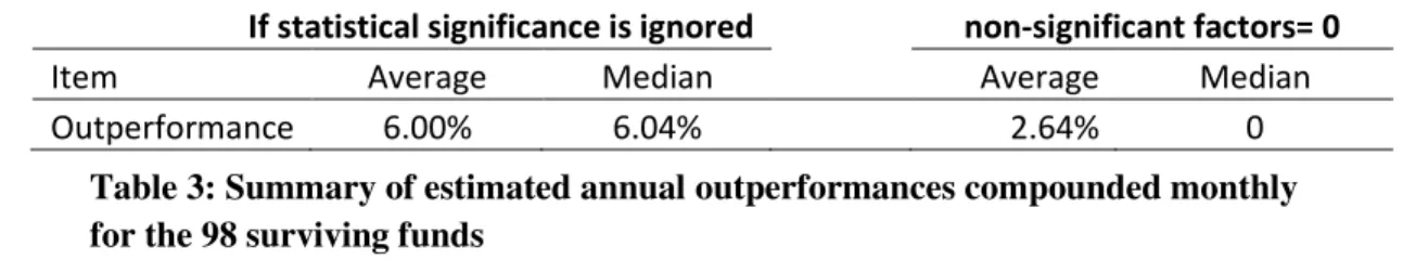
Table 3 gives the average annual outperformances of these funds compounded monthly.
If statistical significance is ignored non-significant factors= 0
Item Average Median Average Median
Outperformance 6.00% 6.04% 2.64% 0
The results from the analysis are quite contrasted. If we ignore the statistical significance of the alphas, we obtain an annual out-performance of 6%. This is higher than the results of the whole
sample. It shows a clear out-performance of the surviving funds compared to the others. If we based our conclusion only on these figures, we would tell that investing in older funds is better than investing in the new ones. However, when we take into account the statistical significance
of the alphas, the findings are completely different. The average annual performance of 2.64% is below the average performance from the full sample of funds. Therefore we cannot conclude
anything from this analysis. However, the values of the market factors were higher in both case (0.17 when we ignore statistical significance and 0.16 otherwise), showing that the returns of these funds are more impacted by the market than the other funds. The TSMOM factors are also
higher in both case (0.03 and 0.02) showing that the use of momentum is still seldom but more
21 important than for general funds. Regarding the other factors, they are able to benefit more from
the commodities in normal backwardation and thanks to their experiences theirs returns are not negatively impacted by commodities in contango and they are even able to make profit from
these commodities depending whether we are ignoring or not the factors’ statistical significance.
c. Time-dependent analyses of the performances
In this sub-section, I analyse the annual performance compounded monthly for the whole sample
for each year of the time period. I will show us how they reacted to the different events that happened during this period such as the crisis in 2007 or the boom of commodities prices in the
early 2000’s. We can expect the funds to out-perform during the crisis period as hedge funds and
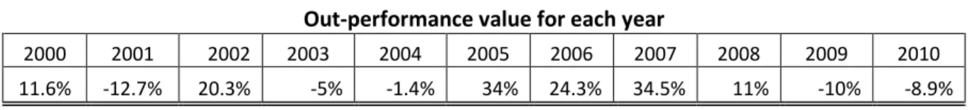
commodities used to. Table 4 shows us the annual out-performance compounded monthly for
each year.
Out-performance value for each year
2000 2001 2002 2003 2004 2005 2006 2007 2008 2009 2010
11.6% -12.7% 20.3% -5% -1.4% 34% 24.3% 34.5% 11% -10% -8.9%
We can clearly see in table 4 that the performances of the funds are highly volatile with quite
often extreme values, either negative as in 2001, 2009 and 2010 or positive like from 2005 to 2007. We can see that during the first half of the decade from 2000 to 2004, the performances
were really disappointing. This period matches with the commodities prices’ boom. Therefore
we can imagine that these poor performances may be linked to the fact that this prosperous period in the commodity market attracted a lot of investors and made it therefore more difficult
to benefit from arbitrages. We can also see that before and during the financial crisis from 2005 to 2007, funds were able to deliver incredibly high returns (around 30% per year). It is perfectly
22 in line with what we were expecting from CTA. However, the results got again negative during
the last 2 years. This volatility shows the riskiness of this market with results that can reach extreme values. We are analysing the persistence of the performances in the next section.
Section 4: The persistence
of the funds’ performance
This section will tackle the persistence of the funds’ performance in order to understand if the
out-performance we witnessed in the previous section is due to mere luck. If the performances
are persistent then it will be the proof that they are due to the skills of the managers but if the performances are really different from one period to another then we can assume that the out-performances may be linked to the mere luck. To analyse the persistence, we will use the
Spearman rank order correlation; the formula is available in the appendix.
a) The persistence of the surviving funds’ performance
We analyse first the persistence of the surviving funds because we expect them to be better than the other funds. Moreover we can assume that if they keep attracting the investors, it may be due
to constant performance. Therefore, we expect the performance of these funds to show a strong and positive persistence.
a. The persistence of the surviving funds’ performance in the long term
In this sub-section, we are going to analyse the persistence of the funds’ performance between the first half of the period and the second half, these two periods are quite long: 5.5 years each.
23 distribution of the ranks for the different funds, we can see that there is no apparent pattern. We
can assume that the periods used to perform the test were too important and therefore not able to capture the persistence. In the next subsection, we see the evolution of the performance for the
surviving funds for shorter periods.
b. The evolution of the performance of the surviving funds’ persistence
Since the periods used for the first Spearman rank order correlation seem too long to capture
correctly the persistence of the funds’ performance, in this section, different time periods will be
used. It will allow us to see the evolution of the persistence according to the time period used and also see if they are confirming the findings of the first section by being all around 0. We can
expect the persistence to decrease while we are increasing the time period because it may be easier to keep out-performing in the short term than in the long term. The graph 3 shows us that
the funds’ performances are definitely not persistent. The short-term persistence is more or less
equal to 0 and become negative in the medium term, showing that the performances are far from
24 being constant and varying a lot from one period to another. We can see that the only positive
coefficient (even if it almost 0) is the coefficient for the persistence between the performance of the first 5.5 years and the performance of the following 6 months. Even in the short term, they
are not able to keep performing. These results contradict our hypothesis that performances are constant thanks to the ability of the CTAs. It is a proof that performances may be linked to mere luck for the surviving funds. In the next subpart, we will tackle the persistence for the
performances of the whole sample, to see if the results are the same or if the surviving funds are not a good representation for the full sample.
b) The persistence for the whole sample
In the previous subsection, we have seen that the performances of the surviving were not
persistent. In this subsection, we are going to see if the conclusions are the same for the whole sample. Since the analysis in the previous subsections showed that using long periods for the Spearman rank order correlation analysis was not providing different conclusions than shorter
0,12
-0,23
-0,47 -0,46
-0,02
-1 -0,8 -0,6 -0,4 -0,2 0 0,2 0,4 0,6 0,8 1
6 months 1 year 2 years 3 years 5.5 years
Persistence
25 periods, in this section we are going to use short periods. Graph 5 shows the persistence of the
funds’ performances between the first half and second half of each year. It will allow us to see if
there is persistence in the short term but also the evolution of the persistence. Having the
persistence for each year will prevent us from drawing conclusions from results of a single time period that could be not fitting the reality.
We can see on graph 5 that the persistence is very volatile from one year to another. The mean seems to be around 0 from 2000 to 2008. As from 2009, the persistence started to stay constant
for 2 years around 0.4, but a 2-years period is too short to assume anything for the future. The graph shows that either the persistence is null or even negative. This clear absence of persistence for the whole sample is in line with the findings from the previous subsection. Thanks to these
different analyses, we can conclude that the performances of the funds are not persistent and
therefore may not be linked to their skills. Since they don’t have the ability to keep a positive
performance, we can assume that the positive performances are due to mere luck.
-1 -0,8 -0,6 -0,4 -0,2 0 0,2 0,4 0,6 0,8 1
Spearman coefficient
26 CONCLUSION:
The goal of this paper was to analyse the performances of the CTA funds and the persistence of the performances in order to get a better understanding of the impact of the skills of the CTAs on
these performances. In the third section, we showed that the CTA funds in average out-performed for the period lasting from 2000 to 2010 no matter if we take into account the significance of the results or not. However, in the fourth section, we noticed that the persistency of the funds’
performances was null or negative. This level of persistency proved that the abilities of the CTAs
are not responsible for the funds’ out-performances, otherwise the funds with best CTAs should
constantly out-perform and the persistency would be strongly positive. The CTAs’ skills don’t seem to have an important impact on the performances of the funds and there is a high volatility of the performances across funds despite the average positive out-performance. These two facts
make questionable the rationale of paying management fees in order to benefit from the management of CTAs. The reasons that could explain why investors are putting more and more
money in these funds are the following: First, it could be due to a lack of information about the real relative performances of such funds and the risks linked to such funds. Investors may see them as relatively safe due to the fact that they involved commodities and professional managers
(the CTAs). The second reason could be that the investors are considering them as high risk/high returns investments. As shown in table 4, the performances reached double digits returns more
than half of the years of the period. The investors would invest in the funds, hoping to invest in the good horse and obtain incredibly high returns. It would be interesting in the future to run again these analyses with a bigger amount of commodities and funds in order to get more