HOLOS, Ano 35, v.2, e8023, 2019 1
PERFIS VERTICAIS DA DENSIDADE E DA TEMPERATURA EM UMA ATMOSFERA DE
VAN DER WAALS NA REGIÃO METROPOLITANA DE NATAL-RN, BRASIL
I. DE M. SILVA*, D. N. SILVA, D. M. MEDEIROS
Atmospheric Research Laboratory, School of Science and Technology, Federal University of Rio Grande do Norte
Artigo submetido em 07/12/2018 e aceito em 24/06/2019 DOI: 10.15628/holos.2019.8023
RESUMO
As constantes 𝑎 e 𝑏 da equação de estado de Van der Waals para atmosfera são determinadas a partir da concentração, da temperatura crítica e da pressão crítica dos gases componentes do ar, usando a regra de mistura de Kay. A radiossonda mede a pressão atmosférica 𝑝, a temperatura 𝑇 e outras variáveis meteorológicas, em vários níveis de altitude. Portanto, a densidade da atmosfera pode ser calculada com base nos parâmetros 𝑎, 𝑏, 𝑝 e 𝑇. Neste estudo, os perfis verticais diurno e noturno da densidade média mensal da atmosfera, na região metropolitana de Natal-RN, Brasil, no período de 2010 a 2017, foram construídos, considerando o sistema atmosférico como um gás ideal e como um gás de Van der Waals. Foram mostrados também os perfis verticais da
diferença da densidade média entre estas duas abordagens e da temperatura. Para o cálculo da densidade nos dois cenários, foram utilizados os dados de radiossonda da atmosfera desta região, com a altitude variando de 50𝑚 até 10𝑘𝑚, interpolados a cada 10𝑚. Verificou-se que a densidade da atmosfera como um gás de Van der Waals apresenta valores mais altos do que a densidade do ar como um gás ideal em baixas altitudes. No entanto, as densidades tendem aos mesmos valores, em ambos os casos, à medida que a altitude aumenta. Mostrou-se ainda uma forte dependência da densidade com a temperatura, tais que as densidades apresentam valores mais elevados nos meses mais frios.
PALAVRAS-CHAVE: Van der Waals, atmosfera, radiossonda, perfil vertical, densidade.
VERTICAL PROFILES OF DENSITY AND TEMPERATURE IN A VAN DER WAALS
ATMOSPHERE IN METROPOLITAN REGION OF NATAL-RN, BRAZIL
ABSTRACT
The constants a and b of the Van der Waals state equation for atmosphere are determined from the concentration, critical temperature and critical pressure of the air components, using the Kay mixing rule. The
radiosonde measures atmospheric pressure 𝑝,
temperature 𝑇 and other meteorological variables at various altitude levels. Therefore, the density of the atmosphere can be calculated based on the parameters 𝑎, 𝑏, 𝑝 and 𝑇. In this study, the diurnal and nocturnal vertical profiles of the monthly average density, in the atmosphere of metropolitan region of Natal-RN, Brazil, from 2010 to 2017, were constructed considering the atmospheric system as an ideal gas and as a Van der
Waals gas. The vertical profiles of the mean density difference between these two approaches and the temperature were also shown. In both scenarios, the radiosonde data of the atmosphere of this region for the calculation of the density were used, with the altitude ranging from 50𝑚 to 10𝑘𝑚, interpolated every 10𝑚. It has verified that the density of the atmosphere as a Van der Waals gas presents values higher than the density of air as an ideal gas at low altitudes. In both cases, densities tend therefore to have the same values when altitude increases. It has also showed a strong dependence on density related to temperature, such that the densities presented higher values in the colder months.
HOLOS, Ano 35, v.2, e8023, 2019 2
1 INTRODUCTION
The gases that constitute the atmosphere are regarded individually as an ideal gas and the mixing of these gases behaves very well when studied by the ideal gas law
𝑝𝑉 = 𝑛𝑅∗𝑇 = 𝑚𝑅𝑇 (1)
In Equation (1) the volume 𝑉 (𝑚3) encloses the mixture under pressure 𝑝 (𝑃𝑎) and temperature 𝑇 (𝐾), 𝑅∗ is the molar gas constant and 𝑅 is the constant for a particular gas, such that the number of moles 𝑛 is the ratio of the mass 𝑚 to the molecular weight 𝑀 of this gas. Therefore, the ideal gas law is always used in the study of the atmosphere, where this equation of state plays an important role in the analysis of thermodynamic properties of this system (Hobbs, 2006).
Johannes Diderik Van der Waals presented in his doctoral thesis in 1873 an equation that considers the intermolecular interactions and corrects the ideal gas law (Nussenzveig, 2000, apud Waals, 1873). In fact, this equation is described by
[𝑝 + 𝑎 (𝑛 𝑉)
2
] [𝑉 − 𝑛𝑏] = 𝑛𝑅∗𝑇 (2)
Here, the 𝑎 (𝐽𝑚3𝑚𝑜𝑙−2) and 𝑏 (𝑚3𝑚𝑜𝑙−1) constants can be determined from the critical
temperature (𝑇𝐶) and the critical pressure (𝑃𝐶) of the studied gas (Smith, 2007). For a Van der
Waals gas, there is a critical point, which corresponds to an inflection point of the pressure-volume-temperature (𝑃𝑉𝑇) curve. Therefore, there is a second order phase transition that implies in the following conditions (𝜕𝑝 𝜕𝑉)𝑇𝐶 = 0 (3) (𝜕 2𝑝 𝜕𝑉2) 𝑇𝐶 = 0 (4)
The solution of the system of equations (2), (3) and (4), relating to the critical properties of the gas, provides the values of 𝑎 and 𝑏, which are written as a function of 𝑇𝐶 and 𝑃𝐶, respectively
𝑎 =27(𝑅 ∗𝑇 𝐶)2 64𝑃𝐶 (5) 𝑏 =𝑅 ∗𝑇 𝐶 8𝑃𝐶 (6)
For a gas mixture the critical properties can be obtained through the group contribution method, and from pseudocritical parameters resulting from the simple rule of linear mixtures, known as the Kay Rule (Daubert, 1989, Jalowka, 1986, Joback, 1983, apud Kay, 1936). This procedure is described by the equation
𝐶𝑃𝑗 = ∑ 𝑋𝑖𝐶𝑃𝑖 𝜅
𝑖
HOLOS, Ano 35, v.2, e8023, 2019 3
In this method, 𝐶𝑃𝑗 represents a critical property of the jth mixture, 𝐶𝑃𝑖 and 𝑋𝑖 are a critical
property and a fraction of the ith component of the mixture, respectively, and 𝜅 is the number of components present in jth mixture.
The rainfall regime over the Northeast of Brazil (NEB) is directly influenced by the general circulation of the atmosphere and by the conditions of the Pacific and Atlantic Oceans (Kane, 1989; Alves et al. 1994; Ferreira e Mello, 2005; Kayano e Andreoli, 2007). The main atmospheric systems operating in this region are the Intertropical Convergence Zone (ITCZ), Upper-Tropospheric Cyclonic Vortex (UTCV), Easterly Waves (EW), Sea and Land Breezes, Cold Fronts, Instability Lines, among others (Ferreira e Mello, 2005). However, the ocean phenomena that influence precipitation over NEB are mainly the El Niño-Southern Oscillation (ENSO) in the Pacific and the Atlantic Dipole (Alves et al. 1994; Kane 1989; Alves et al. 1994; Ferreira e Mello, 2005; Kayano e Andreoli 2007).
Natal is located on the eastern coast of the NEB (05°47'42"S and 35°12'34"W) and washed by the Atlantic Ocean (Figure 1). This city is the largest in the state of Rio Grande do Norte and has approximately 803,739 inhabitants. The metropolitan region of Natal has an area of 3,555.8 𝑘𝑚2 and exceeds the 1.4 million of inhabitants (Natal City Hall, 2010). This region presents a tropical climate with dry summer, such that the rainy season is concentrated from May to July, whereas the dry and intense season is concentrated from September to December (Alvares et. al, 2014).
Atmospheric pressure and temperature are some of the meteorological variables measured by radiosondes, all of which are dependent upon height, such that they provide a vertical profile of these properties (DECEA, 2015). The Augusto Severo Airport is located in the Parnamirim city in the metropolitan region of Natal-RN, Brazil (Figure 1), and launches two daily radiosondes at 00:00 UTC and 12:00 UTC for research purposes (University of Wyoming, 2018).
Figure 1: Augusto Severo Airport, Parnamirim city, metropolitan region of Natal-RN, Brazil. Source: created by the authors. Brazil 80° W 60° W 40° W 30° S 20° S 10° S 0° S NEB RN 50° W 40° W 30° W 15° S 10° S 5° S ● Natal Parnamirim 35.6° W 35.4° W 35.2° W 35° W 6.1° S 6° S 5.9° S 5.8° S 5.7° S
HOLOS, Ano 35, v.2, e8023, 2019 4
Therefore, in this work the data were first obtained from the radiosondes launched at the Augusto Severo Airport, from 2010 to 2017 at 00:00 UTC and 12:00 UTC. In this way, the values of altitude, pressure and temperature, were interpolated for the two daily hours in the metropolitan region of Natal in the last eight years. Following, the variable values at regular altitudes were chosen, that is, for every 10𝑚. Subsequently, the water composition in the atmosphere C%, the critical properties, 𝑇𝐶 and 𝑃𝐶, and the constants 𝑎 and 𝑏 of Van der Waals in this region, from 50𝑚
to 10𝑘𝑚, at each chosen point were computed. The monthly mean air density as an ideal gas and as a Van der Waals gas and the difference between these densities were calculated. Finally, the diurnal and the nocturnal vertical profiles of these properties and temperature in the metropolitan region of Natal were shown and discussed.
2 METHODOLOGY
The ideal gas Equation (1) and the Van der Waals Equation (2) are written in terms of pressure respectively as 𝑝 = (𝑛 𝑉) 𝑅 ∗𝑇 (8) 𝑝 = (𝑛 𝑉) 𝑅 ∗𝑇 + 𝑝𝑏 (𝑛 𝑉) − 𝑎 ( 𝑛 𝑉) 2 − 𝑎𝑏 (𝑛 𝑉) 3 (9)
According to the definition of density 𝜌 ≡ 𝑛/𝑉 in 𝑚𝑜𝑙𝑚−3, the equations (8) and (9) can be written respectively as 𝜌 = 𝑝 𝑅∗𝑇 (10) 𝜌3−1 𝑏𝜌 2+𝑅 ∗𝑇 + 𝑝𝑏 𝑎𝑏 𝜌 − 𝑝 𝑎𝑏 = 0 (11)
The pressure 𝑒 due water vapor is related to the saturation vapor pressure 𝑒𝑠 by the definition of the relative humidity 𝑅𝐻, that is,
𝑅𝐻 = 𝑒
𝑒𝑠× 100 (12)
The water vapor concentration is a highly variable constituent in the atmosphere and is defined according to Dalton's law, such that the percentage water content is
𝐶% =
𝑒
𝑝× 100 (13)
where 𝑝 is the pressure of the air. When 𝑒 > 𝑒𝑠 then the water condenses, which usually
occurs in cooling the air. In this case, the saturation vapor pressure 𝑒𝑠 will be greater as much as
the temperature 𝑇 is higher.
The empirical formula that is used to calculate 𝑒𝑠 is the Tetens equation (Huang, 2018, apud
Tetens, 1930)
𝑒𝑠 = 𝐴 exp ( 17.3 𝑡
HOLOS, Ano 35, v.2, e8023, 2019 5
where the parameter 𝐴 used is 610.8 𝑃𝑎 or 4.58 𝑚𝑚𝐻𝑔. Combination of Equations (12), (13) and (14) yields 𝐶% = 𝑅𝐻 𝑝 610.8 exp ( 17.3 𝑡 237.3 + 𝑡) (15)
where 𝑅𝐻, 𝑝, and 𝑡 are, respectively, the relative humidity in %, the pressure of air in 𝑃𝑎, and the temperature in ℃.
Initially, the daily values of 𝑝, 𝑇 and 𝑅𝐻, measured by the radiosonde at 00:00 UTC and at 12:00 UTC, from 2010 to 2017, in the atmosphere above the metropolitan region of Natal-RN, Brazil, were used. These data were interpolated to the values corresponding to regular altitudes every 10𝑚. From these results, the concentration of the water 𝐶% was calculated at each height
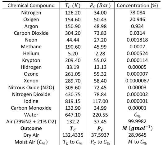
by Equation (15) and inserted in Table I. The critical temperature 𝑇𝐶 and critical pressure 𝑃𝐶 for those heights were computed through the Kay rule and Table I, and the values of the Van der Waals constants 𝑎 and 𝑏 calculated by Equations (5) and (6).
From the data of 𝑝 and 𝑇 for the previous altitudes, the density 𝜌 of the atmosphere was determined as the ideal gas at each point through the Equation (10). Here, all the results are multiplied by molar mass 𝑀 (Table I), to obtain the density 𝜌 in 𝑔𝑚−3.
Table I: Critical parameters and the composition of atmospheric (Trace Gases, 2010, NASA, 2016).
Chemical Compound 𝑇𝐶 (𝐾) 𝑃𝐶 (𝐵𝑎𝑟) Concentration (%)
Nitrogen Oxigen Argon Carbon Dioxide Neon Methane Helium Krypton Hidrogen Ozone Xenon Nitrous Oxide (N2O)
Nitrogen Dioxide Iodine Carbon Monoxide Water Air (79%N2 + 21% O2) Outcome Dry Air Moist Air (𝐶%) 126.20 154.60 150.90 304.20 44.44 190.60 5.20 209.40 33.19 261.05 289.70 309.60 430.75 819.15 132.90 647.10 132.2 𝑻𝑪 132,4335 𝑇𝐶 to 𝐶% 34.00 50.43 48.98 73.83 27.20 45.99 2.28 55.02 13.13 55.32 58.40 72.45 78.84 117.00 34.99 220.55 37.45 𝑷𝑪 37,5937 𝑃𝐶 to 𝐶% 78.084 20.946 0.934 0.0314 0.001818 0.0002 0.000524 0.000114 0.00005 0.000007 0.0000087 0.00003 0.000002 0.000001 0.00001 𝐶% 99.9982 𝑴 (𝒈𝒎𝒐𝒍−𝟏) 28,9645 𝑀 to 𝐶%
The Equation (11) was solved for all previous altitudes, from the data of 𝑝 and 𝑇, and all 𝑎 and 𝑏 values according to the Table I. Two roots of this equation were complex and one was real, for every point. Therefore, the density of the atmosphere as a Van der Waals gas was calculated by the real solution, which is the one that has physical significance. All values are multiplied by molar mass 𝑀 (Table I), to obtain the density in 𝑔𝑚−3. Subsequently, the monthly averages of
HOLOS, Ano 35, v.2, e8023, 2019 6
densities were calculated at all regular altitudes. Finally, the difference ∆ between the average monthly densities obtained for the Van der Waals atmosphere and the ideal gas air was evaluated. As such, this research was conducted to construct the vertical profiles of diurnal and nocturnal of the monthly average density in the atmosphere of the metropolitan region of Natal-RN, Brazil, as an ideal gas and as a Van der Waals gas, from 2010 to 2017, with the altitude varying regularly every 10𝑚, from 50𝑚 to 10𝑘𝑚. The vertical profile of the difference between the average monthly densities obtained for the Van der Waals atmosphere and the ideal gas was made. The vertical profile of the temperature was also drawn, to assist in understanding the densities outcomes.
3 RESULTS AND DISCUSSION
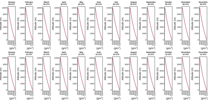
The vertical profiles of the monthly mean density 𝜌 in the atmosphere of the metropolitan region of Natal-RN, at 00:00 UTC and 12:00 UTC are shown in Figures 2 and 3, from 2010 to 2017. The densities as ideal gas and as Van der Waals gas were studied from 50𝑚 to 10𝑘𝑚 (Figure 2) and from 50𝑚 to 100𝑚 (Figure 3). It was observed in Figure 2 that the both air densities decreases linearly with the altitude in diurnal and nocturnal periods, from a value of approximately 1200𝑔𝑚−3 close to the surface up to a value of 400𝑔𝑚−3 at the 10𝑘𝑚 altitude.
Figure 2: Vertical profiles of the monthly mean density 𝝆 in the atmosphere in Natal-RN, at 00:00 UTC and 12:00 UTC, from 𝟓𝟎𝒎 to 𝟏𝟎𝒌𝒎. Red and blue lines correspond to Van der Waals gas and ideal gas respectively. Source: created by the authors.
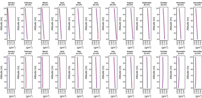
The density profiles from 50𝑚 to 100𝑚 showed that the values of ρ in the Van der Waals atmosphere are slightly higher than in the ideal gas air (Figure 3). This probably occurs because the concentration of the water in the atmosphere of the study region is higher near the surface, reaching values close to 3%. Also in Figure 3, it was observed that the ranges with the highest values of density close to the surface are in June, July and August, for the two daily times.
The difference ∆ between the average monthly densities in the Van der Waals atmosphere and in the ideal gas air were considered from 50𝑚 to 10𝑘𝑚 in Figure 4, and from 50𝑚 to 100𝑚 in Figure 5. A similar pattern for all months in both atmospheric gas approaches was showed in
4 0 0 6 0 0 8 0 0 1 0 0 0 1 2 0 0 0 2000 4000 6000 8000 10000 r (g/m3 ) A lt it u d e ( m ) January 00 UTC 4 0 0 6 0 0 8 0 0 1 0 0 0 1 2 0 0 0 2000 4000 6000 8000 10000 r (g/m3 ) A lt it u d e ( m ) February 00 UTC 4 0 0 6 0 0 8 0 0 1 0 0 0 1 2 0 0 0 2000 4000 6000 8000 10000 r (g/m3 ) A lt it u d e ( m ) March 00 UTC 4 0 0 6 0 0 8 0 0 1 0 0 0 1 2 0 0 0 2000 4000 6000 8000 10000 r (g/m3 ) A lt it u d e ( m ) April 00 UTC 4 0 0 6 0 0 8 0 0 1 0 0 0 1 2 0 0 0 2000 4000 6000 8000 10000 r (g/m3 ) A lt it u d e ( m ) May 00 UTC 4 0 0 6 0 0 8 0 0 1 0 0 0 1 2 0 0 0 2000 4000 6000 8000 10000 r (g/m3 ) A lt it u d e ( m ) June 00 UTC 4 0 0 6 0 0 8 0 0 1 0 0 0 1 2 0 0 0 2000 4000 6000 8000 10000 r (g/m3 ) A lt it u d e ( m ) July 00 UTC 4 0 0 6 0 0 8 0 0 1 0 0 0 1 2 0 0 0 2000 4000 6000 8000 10000 r (g/m3 ) A lt it u d e ( m ) August 00 UTC 4 0 0 6 0 0 8 0 0 1 0 0 0 1 2 0 0 0 2000 4000 6000 8000 10000 r (g/m3 ) A lt it u d e ( m ) September 00 UTC 4 0 0 6 0 0 8 0 0 1 0 0 0 1 2 0 0 0 2000 4000 6000 8000 10000 r (g/m3 ) A lt it u d e ( m ) October 00 UTC 4 0 0 6 0 0 8 0 0 1 0 0 0 1 2 0 0 0 2000 4000 6000 8000 10000 r (g/m3 ) A lt it u d e ( m ) November 00 UTC 4 0 0 6 0 0 8 0 0 1 0 0 0 1 2 0 0 0 2000 4000 6000 8000 10000 r (g/m3 ) A lt it u d e ( m ) December 00 UTC 4 0 0 6 0 0 8 0 0 1 0 0 0 1 2 0 0 0 2000 4000 6000 8000 10000 r (g/m3 ) A lt it u d e ( m ) January 12 UTC 4 0 0 6 0 0 8 0 0 1 0 0 0 1 2 0 0 0 2000 4000 6000 8000 10000 r (g/m3 ) A lt it u d e ( m ) February 12 UTC 4 0 0 6 0 0 8 0 0 1 0 0 0 1 2 0 0 0 2000 4000 6000 8000 10000 r (g/m3 ) A lt it u d e ( m ) March 12 UTC 4 0 0 6 0 0 8 0 0 1 0 0 0 1 2 0 0 0 2000 4000 6000 8000 10000 r (g/m3 ) A lt it u d e ( m ) April 12 UTC 4 0 0 6 0 0 8 0 0 1 0 0 0 1 2 0 0 0 2000 4000 6000 8000 10000 r (g/m3 ) A lt it u d e ( m ) May 12 UTC 4 0 0 6 0 0 8 0 0 1 0 0 0 1 2 0 0 0 2000 4000 6000 8000 10000 r (g/m3 ) A lt it u d e ( m ) June 12 UTC 4 0 0 6 0 0 8 0 0 1 0 0 0 1 2 0 0 0 2000 4000 6000 8000 10000 r (g/m3 ) A lt it u d e ( m ) July 12 UTC 4 0 0 6 0 0 8 0 0 1 0 0 0 1 2 0 0 0 2000 4000 6000 8000 10000 r (g/m3 ) A lt it u d e ( m ) August 12 UTC 4 0 0 6 0 0 8 0 0 1 0 0 0 1 2 0 0 0 2000 4000 6000 8000 10000 r (g/m3 ) A lt it u d e ( m ) September 12 UTC 4 0 0 6 0 0 8 0 0 1 0 0 0 1 2 0 0 0 2000 4000 6000 8000 10000 r (g/m3 ) A lt it u d e ( m ) October 12 UTC 4 0 0 6 0 0 8 0 0 1 0 0 0 1 2 0 0 0 2000 4000 6000 8000 10000 r (g/m3 ) A lt it u d e ( m ) November 12 UTC 4 0 0 6 0 0 8 0 0 1 0 0 0 1 2 0 0 0 2000 4000 6000 8000 10000 r (g/m3 ) A lt it u d e ( m ) December 12 UTC
HOLOS, Ano 35, v.2, e8023, 2019 7
graphs in Figure 4. However, a different behavior pattern every month near the surface is shown in Figure 5. In this case, July at 00:00 UTC was highlighted, since this month presented the highest values of 𝜌. Also in Figures 4 and 5, it was noted that the density of the Van der Waals atmosphere is approximately 1.14𝑔𝑚−3 higher than the density of ideal gas air near the surface. This change is an order of magnitude greater than that in the end of the 10𝑘𝑚 altitude, which is approximately 0.1𝑔𝑚−3.
Figure 3: Vertical profiles of the monthly mean density 𝝆 in the atmosphere in Natal-RN, at 00:00 UTC and 12:00 UTC, from 𝟓𝟎𝒎 to 𝟏𝟎𝟎𝒎. Red and blue lines correspond to Van der Waals gas and ideal gas respectively. Source: created by the authors.
Figure 4: The difference ∆ between the average monthly densities in the Van der Waals atmosphere and in the ideal gas air in Natal-RN, at 00:00 UTC and 12:00 UTC, from 𝟓𝟎𝒎 to 𝟏𝟎𝒌𝒎. Source: created by the authors.
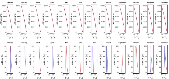
The vertical profiles of the average monthly temperature 𝑇 at 00:00 UTC and 12:00 UTC are also constructed from 50𝑚 to 10𝑘𝑚 and from 50𝑚 to 100𝑚 in Figure 6. The temperature was decreased linearly with the altitude, reaching values little less than −30℃ in the altitude of 10𝑘𝑚 and values close to 30℃ in the altitude of 50𝑚. The vertical profiles of diurnal and nocturnal from
50 60 70 80 90 100 r (g/m3 ) A lt it u d e ( m ) January 00 UTC 1 1 6 0 1 1 6 8 1 1 7 6 1 1 8 4 50 60 70 80 90 100 r (g/m3 ) A lt it u d e ( m ) February 00 UTC 1 1 6 0 1 1 6 8 1 1 7 6 1 1 8 4 50 60 70 80 90 100 r (g/m3 ) A lt it u d e ( m ) March 00 UTC 1 1 6 0 1 1 6 8 1 1 7 6 1 1 8 4 50 60 70 80 90 100 r (g/m3 ) A lt it u d e ( m ) April 00 UTC 1 1 6 0 1 1 6 8 1 1 7 6 1 1 8 4 50 60 70 80 90 100 r (g/m3 ) A lt it u d e ( m ) May 00 UTC 1 1 6 0 1 1 6 8 1 1 7 6 1 1 8 4 50 60 70 80 90 100 r (g/m3 ) A lt it u d e ( m ) June 00 UTC 1 1 6 0 1 1 6 8 1 1 7 6 1 1 8 4 50 60 70 80 90 100 r (g/m3 ) A lt it u d e ( m ) July 00 UTC 1 1 6 0 1 1 6 8 1 1 7 6 1 1 8 4 50 60 70 80 90 100 r (g/m3 ) A lt it u d e ( m ) August 00 UTC 1 1 6 0 1 1 6 8 1 1 7 6 1 1 8 4 50 60 70 80 90 100 r (g/m3 ) A lt it u d e ( m ) September 00 UTC 1 1 6 0 1 1 6 8 1 1 7 6 1 1 8 4 50 60 70 80 90 100 r (g/m3 ) A lt it u d e ( m ) October 00 UTC 1 1 6 0 1 1 6 8 1 1 7 6 1 1 8 4 50 60 70 80 90 100 r (g/m3 ) A lt it u d e ( m ) November 00 UTC 1 1 6 0 1 1 6 8 1 1 7 6 1 1 8 4 50 60 70 80 90 100 r (g/m3 ) A lt it u d e ( m ) December 00 UTC 1 1 6 0 1 1 6 8 1 1 7 6 1 1 8 4 50 60 70 80 90 100 r (g/m3 ) A lt it u d e ( m ) January 12 UTC 1 1 6 0 1 1 6 8 1 1 7 6 1 1 8 4 50 60 70 80 90 100 r (g/m3 ) A lt it u d e ( m ) February 12 UTC 1 1 6 0 1 1 6 8 1 1 7 6 1 1 8 4 50 60 70 80 90 100 r (g/m3 ) A lt it u d e ( m ) March 12 UTC 1 1 6 0 1 1 6 8 1 1 7 6 1 1 8 4 50 60 70 80 90 100 r (g/m3 ) A lt it u d e ( m ) April 12 UTC 1 1 6 0 1 1 6 8 1 1 7 6 1 1 8 4 50 60 70 80 90 100 r (g/m3 ) A lt it u d e ( m ) May 12 UTC 1 1 6 0 1 1 6 8 1 1 7 6 1 1 8 4 50 60 70 80 90 100 r (g/m3 ) A lt it u d e ( m ) June 12 UTC 1 1 6 0 1 1 6 8 1 1 7 6 1 1 8 4 50 60 70 80 90 100 r (g/m3 ) A lt it u d e ( m ) July 12 UTC 1 1 6 0 1 1 6 8 1 1 7 6 1 1 8 4 50 60 70 80 90 100 r (g/m3 ) A lt it u d e ( m ) August 12 UTC 1 1 6 0 1 1 6 8 1 1 7 6 1 1 8 4 50 60 70 80 90 100 r (g/m3 ) A lt it u d e ( m ) September 12 UTC 1 1 6 0 1 1 6 8 1 1 7 6 1 1 8 4 50 60 70 80 90 100 r (g/m3 ) A lt it u d e ( m ) October 12 UTC 1 1 6 0 1 1 6 8 1 1 7 6 1 1 8 4 50 60 70 80 90 100 r (g/m3 ) A lt it u d e ( m ) November 12 UTC 1 1 6 0 1 1 6 8 1 1 7 6 1 1 8 4 50 60 70 80 90 100 r (g/m3 ) A lt it u d e ( m ) December 12 UTC 1 1 6 0 1 1 6 8 1 1 7 6 1 1 8 4 0 2000 4000 6000 8000 10000 D (g/m3 ) A lt it u d e ( m ) January 00 UTC 0 .1 0 .4 0 .7 1 .0 0 2000 4000 6000 8000 10000 D (g/m3 ) A lt it u d e ( m ) February 00 UTC 0 .1 0 .4 0 .7 1 .0 0 2000 4000 6000 8000 10000 D (g/m3 ) A lt it u d e ( m ) March 00 UTC 0 .1 0 .4 0 .7 1 .0 0 2000 4000 6000 8000 10000 D (g/m3 ) A lt it u d e ( m ) April 00 UTC 0 .1 0 .4 0 .7 1 .0 0 2000 4000 6000 8000 10000 D (g/m3 ) A lt it u d e ( m ) May 00 UTC 0 .1 0 .4 0 .7 1 .0 0 2000 4000 6000 8000 10000 D (g/m3 ) A lt it u d e ( m ) June 00 UTC 0 .1 0 .4 0 .7 1 .0 0 2000 4000 6000 8000 10000 D (g/m3 ) A lt it u d e ( m ) July 00 UTC 0 .1 0 .4 0 .7 1 .0 0 2000 4000 6000 8000 10000 D (g/m3 ) A lt it u d e ( m ) August 00 UTC 0 .1 0 .4 0 .7 1 .0 0 2000 4000 6000 8000 10000 D (g/m3 ) A lt it u d e ( m ) September 00 UTC 0 .1 0 .4 0 .7 1 .0 0 2000 4000 6000 8000 10000 D (g/m3 ) A lt it u d e ( m ) October 00 UTC 0 .1 0 .4 0 .7 1 .0 0 2000 4000 6000 8000 10000 D (g/m3 ) A lt it u d e ( m ) November 00 UTC 0 .1 0 .4 0 .7 1 .0 0 2000 4000 6000 8000 10000 D (g/m3 ) A lt it u d e ( m ) December 00 UTC 0 .1 0 .4 0 .7 1 .0 0 2000 4000 6000 8000 10000 D (g/m3 ) A lt it u d e ( m ) January 12 UTC 0 .1 0 .4 0 .7 1 .0 0 2000 4000 6000 8000 10000 D (g/m3 ) A lt it u d e ( m ) February 12 UTC 0 .1 0 .4 0 .7 1 .0 0 2000 4000 6000 8000 10000 D (g/m3 ) A lt it u d e ( m ) March 12 UTC 0 .1 0 .4 0 .7 1 .0 0 2000 4000 6000 8000 10000 D (g/m3 ) A lt it u d e ( m ) April 12 UTC 0 .1 0 .4 0 .7 1 .0 0 2000 4000 6000 8000 10000 D (g/m3 ) A lt it u d e ( m ) May 12 UTC 0 .1 0 .4 0 .7 1 .0 0 2000 4000 6000 8000 10000 D (g/m3 ) A lt it u d e ( m ) June 12 UTC 0 .1 0 .4 0 .7 1 .0 0 2000 4000 6000 8000 10000 D (g/m3 ) A lt it u d e ( m ) July 12 UTC 0 .1 0 .4 0 .7 1 .0 0 2000 4000 6000 8000 10000 D (g/m3 ) A lt it u d e ( m ) August 12 UTC 0 .1 0 .4 0 .7 1 .0 0 2000 4000 6000 8000 10000 D (g/m3 ) A lt it u d e ( m ) September 12 UTC 0 .1 0 .4 0 .7 1 .0 0 2000 4000 6000 8000 10000 D (g/m3 ) A lt it u d e ( m ) October 12 UTC 0 .1 0 .4 0 .7 1 .0 0 2000 4000 6000 8000 10000 D (g/m3 ) A lt it u d e ( m ) November 12 UTC 0 .1 0 .4 0 .7 1 .0 0 2000 4000 6000 8000 10000 D (g/m3 ) A lt it u d e ( m ) December 12 UTC 0 .1 0 .4 0 .7 1 .0
HOLOS, Ano 35, v.2, e8023, 2019 8
50𝑚 to 100𝑚 shows that the temperature at 12:00 UTC is higher than 00:00 UTC. Figure 6 is shown that the temperatures in two times are approaching the same value with the increase of altitude, and they practically become equal from 100𝑚. Figures 3 and 6 are also shown that the coldest months of the year, i. e., June, July and August, correspond to the period with the highest density. On the other hand, the hottest months of the year, i. e., December, January and February, correspond to the period with the lowest density. These results reinforce the density dependence relating to temperature.
Figure 5: The difference ∆ between the average monthly densities in the Van der Waals atmosphere and in the ideal gas air in Natal-RN, at 00:00 UTC and 12:00 UTC, from 𝟓𝟎𝒎 to 𝟏𝟎𝟎𝒎. Source: created by the authors.
Figure 6: Vertical profiles of the monthly mean temperature 𝑻 in the atmosphere in Natal-RN, from 𝟓𝟎𝒎 to 𝟏𝟎𝒌𝒎 and from 𝟓𝟎𝒎 to 𝟏𝟎𝟎𝒎. Blue and red lines correspond to 00:00 UTC and 12:00 UTC respectively. Source: created by the authors. 50 60 70 80 90 100 D (g/m3 ) A lt it u d e ( m ) January 00 UTC 1 .0 6 1 .0 8 1 .1 0 1 .1 2 1 .1 4 50 60 70 80 90 100 D (g/m3 ) A lt it u d e ( m ) February 00 UTC 1 .0 6 1 .0 8 1 .1 0 1 .1 2 1 .1 4 50 60 70 80 90 100 D (g/m3 ) A lt it u d e ( m ) March 00 UTC 1 .0 6 1 .0 8 1 .1 0 1 .1 2 1 .1 4 50 60 70 80 90 100 D (g/m3 ) A lt it u d e ( m ) April 00 UTC 1 .0 6 1 .0 8 1 .1 0 1 .1 2 1 .1 4 50 60 70 80 90 100 D (g/m3 ) A lt it u d e ( m ) May 00 UTC 1 .0 6 1 .0 8 1 .1 0 1 .1 2 1 .1 4 50 60 70 80 90 100 D (g/m3 ) A lt it u d e ( m ) June 00 UTC 1 .0 6 1 .0 8 1 .1 0 1 .1 2 1 .1 4 50 60 70 80 90 100 D (g/m3 ) A lt it u d e ( m ) July 00 UTC 1 .0 6 1 .0 8 1 .1 0 1 .1 2 1 .1 4 50 60 70 80 90 100 D (g/m3 ) A lt it u d e ( m ) August 00 UTC 1 .0 6 1 .0 8 1 .1 0 1 .1 2 1 .1 4 50 60 70 80 90 100 D (g/m3 ) A lt it u d e ( m ) September 00 UTC 1 .0 6 1 .0 8 1 .1 0 1 .1 2 1 .1 4 50 60 70 80 90 100 D (g/m3 ) A lt it u d e ( m ) October 00 UTC 1 .0 6 1 .0 8 1 .1 0 1 .1 2 1 .1 4 50 60 70 80 90 100 D (g/m3 ) A lt it u d e ( m ) November 00 UTC 1 .0 6 1 .0 8 1 .1 0 1 .1 2 1 .1 4 50 60 70 80 90 100 D (g/m3 ) A lt it u d e ( m ) December 00 UTC 1 .0 6 1 .0 8 1 .1 0 1 .1 2 1 .1 4 50 60 70 80 90 100 D (g/m3 ) A lt it u d e ( m ) January 12 UTC 1 .0 6 1 .0 8 1 .1 0 1 .1 2 1 .1 4 50 60 70 80 90 100 D (g/m3 ) A lt it u d e ( m ) February 12 UTC 1 .0 6 1 .0 8 1 .1 0 1 .1 2 1 .1 4 50 60 70 80 90 100 D (g/m3 ) A lt it u d e ( m ) March 12 UTC 1 .0 6 1 .0 8 1 .1 0 1 .1 2 1 .1 4 50 60 70 80 90 100 D (g/m3 ) A lt it u d e ( m ) April 12 UTC 1 .0 6 1 .0 8 1 .1 0 1 .1 2 1 .1 4 50 60 70 80 90 100 D (g/m3 ) A lt it u d e ( m ) May 12 UTC 1 .0 6 1 .0 8 1 .1 0 1 .1 2 1 .1 4 50 60 70 80 90 100 D (g/m3 ) A lt it u d e ( m ) June 12 UTC 1 .0 6 1 .0 8 1 .1 0 1 .1 2 1 .1 4 50 60 70 80 90 100 D (g/m3 ) A lt it u d e ( m ) July 12 UTC 1 .0 6 1 .0 8 1 .1 0 1 .1 2 1 .1 4 50 60 70 80 90 100 D (g/m3 ) A lt it u d e ( m ) August 12 UTC 1 .0 6 1 .0 8 1 .1 0 1 .1 2 1 .1 4 50 60 70 80 90 100 D (g/m3 ) A lt it u d e ( m ) September 12 UTC 1 .0 6 1 .0 8 1 .1 0 1 .1 2 1 .1 4 50 60 70 80 90 100 D (g/m3 ) A lt it u d e ( m ) October 12 UTC 1 .0 6 1 .0 8 1 .1 0 1 .1 2 1 .1 4 50 60 70 80 90 100 D (g/m3 ) A lt it u d e ( m ) November 12 UTC 1 .0 6 1 .0 8 1 .1 0 1 .1 2 1 .1 4 50 60 70 80 90 100 D (g/m3 ) A lt it u d e ( m ) December 12 UTC 1 .0 6 1 .0 8 1 .1 0 1 .1 2 1 .1 4 −30 10 0 2000 4000 6000 8000 10000 T (°C) A lt it u d e ( m ) January −30 10 0 2000 4000 6000 8000 10000 T (°C) A lt it u d e ( m ) February −30 10 0 2000 4000 6000 8000 10000 T (°C) A lt it u d e ( m ) March −30 10 0 2000 4000 6000 8000 10000 T (°C) A lt it u d e ( m ) April −30 10 0 2000 4000 6000 8000 10000 T (°C) A lt it u d e ( m ) May −30 10 0 2000 4000 6000 8000 10000 T (°C) A lt it u d e ( m ) June −30 10 0 2000 4000 6000 8000 10000 T (°C) A lt it u d e ( m ) July −30 10 0 2000 4000 6000 8000 10000 T (°C) A lt it u d e ( m ) August −30 10 0 2000 4000 6000 8000 10000 T (°C) A lt it u d e ( m ) September −30 10 0 2000 4000 6000 8000 10000 T (°C) A lt it u d e ( m ) October −30 10 0 2000 4000 6000 8000 10000 T (°C) A lt it u d e ( m ) November −30 10 0 2000 4000 6000 8000 10000 T (°C) A lt it u d e ( m ) December 23 27 50 60 70 80 90 100 T (°C) A lt it u d e ( m ) January 23 27 50 60 70 80 90 100 T (°C) A lt it u d e ( m ) February 23 27 50 60 70 80 90 100 T (°C) A lt it u d e ( m ) March 23 27 50 60 70 80 90 100 T (°C) A lt it u d e ( m ) April 23 27 50 60 70 80 90 100 T (°C) A lt it u d e ( m ) May 23 27 50 60 70 80 90 100 T (°C) A lt it u d e ( m ) June 23 27 50 60 70 80 90 100 T (°C) A lt it u d e ( m ) July 23 27 50 60 70 80 90 100 T (°C) A lt it u d e ( m ) August 23 27 50 60 70 80 90 100 T (°C) A lt it u d e ( m ) September 23 27 50 60 70 80 90 100 T (°C) A lt it u d e ( m ) October 23 27 50 60 70 80 90 100 T (°C) A lt it u d e ( m ) November 23 27 50 60 70 80 90 100 T (°C) A lt it u d e ( m ) December
HOLOS, Ano 35, v.2, e8023, 2019 9
4 CONCLUSIONS
The atmosphere of the metropolitan region of Natal was studied as ideal gas and as Van der Waals gas, from radiosonde data, from 2010 to 2017 at 00:00 UTC and 12:00 UTC. In this context, the monthly mean density profiles for each gas, for the difference between the two monthly mean densities and for the temperature, were constructed from 50𝑚 to 100𝑚 and from 50𝑚 to 10𝑘𝑚. In general, we have demonstrated that the density in both gas approaches, and the temperature, decrease linearly with the altitude in diurnal and nocturnal periods, confirming the density dependence relating to temperature. In addition, the density increases in the cold months, whereas decreases in the warm months. We have also noted that the density in the Van der Waals atmosphere is slightly higher than in the ideal gas air. This probably occurs because the concentration of the water in the atmosphere of this region is higher, as well as the molecular interaction between the air gases is intense, near the surface. The density of the Van der Waals atmosphere is approximately 1.14𝑔𝑚−3 higher than the density of ideal gas air near the surface, and this change is approximately 0.1𝑔𝑚−3 in the 10𝑘𝑚 altitude. Although that value closest to the surface is an apparently small difference between the densities of Van der Waals and of ideal gas for atmosphere, we believe that there is relevant to consider the air as a Van der Waals gas in studying projectile and rocket launches. To justify this, we can state that the drag force acting on the projectile, or rocket, which is one of the component forces acting in the direction of the motion, depends linearly on the density of air. Therefore, we recommend a meticulous study of the density to the atmosphere like a Van der Waals gas, mainly closer to the Earth's surface, increasing the accuracy on projectile and rocket launches. Moreover, this proposal may increase the accuracy in the projectile and rocket launches, both in calculating the quantity of fuel used and in determining the altitude reached.
5 REFERENCES
Alvares, C. A., Stape, J. L. & Sentelhas, P. C. (2014). Köppen’s climate classification map for Brazil. Meteorologische Zeitschrift, vol. 22, n. 6, pp. 711-728. doi: 10.1127/0941-2948/2013/0507.
Alves, J. M. B., Repelli, C. A. & Mello, N. G. (1994). A pré-estação chuvosa do setor Norte da região
Nordeste do Brasil (NEB) e a sua relação com a temperatura dos oceanos adjacentes. Revista
Brasileira de Meteorologia (Impresso), São Paulo, vol. 8, n. 1, pp. 22-30.
Ferreira, A. G. & Mello, N. G. da S. (2005). Principais sistemas atmosféricos atuantes sobre a região
Nordeste do Brasil e a influência dos Oceanos Pacíficos e Atlânticos no clima da região. Revista
Brasileira de Climatologia, vol. 1, n. 1, pp. 15-28. doi:
http://dx.doi.org/10.5380/abclima.v1i1.25215.
Daubert, T. E. & Bartakovits, R. (1989). Prediction of Critical Temperature and Pressure of Organic
Compounds by Group Contribution. Ind. Eng. Chem. Res., vol. 28, pp. 638.
Hobbs, P. V., & Wallace, J. M. (2006). Atmospheric Science: an introductory survey. San Diego: Elsevier.
HOLOS, Ano 35, v.2, e8023, 2019 10
Huang, P. (2018). A Simple Accurate Formula for Calculating Saturation Vapor Pressure of Water
and Ice. J. Appl. Meteor. Climatol., 57, 1265–1272.
Jalowka, J. W. & Daubert, T. E. (1986). Group Contribution Method to Predict Critical Temperature
and Pressure of Hydrocarbons. Ind. Eng. Process Des. Dev., vol. 25, pp.139.
Joback, K. G. & Reid, R. C. (1983). Estimation of Pure-Component Properties from Group
Contributions. Chem. Eng. Cornmun., vol. 57, pp. 233, 1983.
Kane, R. P. (1989). Relationship between the southern oscillation/El Niño and rainfall in some
tropical and midlatitude regions. Proc. Indian Acad. Sci. (Earth Planet Sci.), vol. 98, n. 3, pp.
223-235. doi:10.1007/BF02881825.
Kay, W. B. (1936). Density of Hydrocarbon Gases and Vapors, Ind. Eng. Chem., 28, 9, pp. 1014-1019. Kayano, M. T. & Andreoli, R. V. (2007). Relations of South American summer rainfall interannual
variations with the Pacific decadal oscillation. Inter. J. of Climat., vol. 27, pp. 531-540.
doi:10.1002/joc.1417.
Manual de Estações Meteorológicas de Altitude, Departamento de Controle do Espaço Aéreo (DECEA), Ministério da Defesa Comando da Aeronáutica (2015). Available: https://publicacoes.decea.gov.br/?i=publicacao&id=4282.
NASA, Earth Fact Sheet (2016). Available:
http://nssdc.gsfc.nasa.gov/planetary/factsheet/earthfact.html.
Natal City Hall, Conheça melhor Natal e região metropolitana (2010). Available: https://natal.rn.gov.br/.
Nussenzveig, H. M. (2000). Curso de Física Básica: 2 - Fluidos, Oscilações e Ondas, Calor. São Paulo: Editora Edgard Blücher LTDA.
Smith, J. M., Van Ness, H. C. & Abbott, M. M. (2007). Introdução à Termodinâmica da Engenharia
Química, Brasil: LTC.
Tetens, V. O. (1930). Uber einige meteorologische Begriffe. Zeitschrift Geophysic, v. 6, pp. 297-309.
Trace Gases. Originally (2010). Available:
http://www.ace.mmu.ac.uk/eae/atmosphere/older/Trace_Gases.html. Available:
https://web.archive.org/web/20101009044345/
University of Wyoming, 2018. Available: http://weather.uwyo.edu/upperair/sounding.html Van der Waals, J. D. (1873). On the Continuity of the Gaseous and Liquid States Doctoral Dissertation, Leiden University, Leiden, Netherland.