arXiv:1601.07592v1 [math.OC] 27 Jan 2016
Non-asymptotic confidence bounds for the optimal value of a
stochastic program
Vincent Guigues ∗ Anatoli Juditsky † Arkadi Nemirovski ‡
Abstract
We discuss a general approach to building non-asymptotic confidence bounds for stochas-tic optimization problems. Our principal contribution is the observation that a Sample Av-erage Approximation of a problem supplies upper and lower bounds for the optimal value of the problem which are essentially better than the quality of the corresponding optimal solu-tions. At the same time, such bounds are more reliable than “standard” confidence bounds obtained through the asymptotic approach. We also discuss bounding the optimal value of MinMax Stochastic Optimization and stochastically constrained problems. We conclude with a small simulation study illustrating the numerical behavior of the proposed bounds.
Keywords: Sample Average Approximation; confidence interval; MinMax Stochastic Opti-mization; stochastically constrained problems.
1
Introduction
Consider the following Stochastic Programming (SP) problem
Opt = min
x [f(x) =E{F(x, ξ)}, x∈X] (1)
whereX⊂Rnis a nonempty bounded closed convex set,ξ is a random vector with probability distribution P on Ξ ⊂ Rk and F : X ×Ξ → R. There are two competing approaches for solving (1) when a sample ξN = (ξ1, ..., ξN) of realizations of ξ (or a device to sample from
the distribution P) is available — Sample Average Approximation (SAA) and the Stochastic Approximation (SA). The basic idea of the SAA method is to build an approximation of the “true” problem (1) by replacing the expectation f(x) with its sample average approximation
fN(x) =
1
N N
X
t=1
F(x, ξt), x∈X.
∗FGV/EMAp, 190 Praia de Botafogo, Botafogo, 22250-900 Rio de Janeiro, Brazil,[email protected] †LJK, Universit´e Grenoble Alpes, B.P. 53, 38041 Grenoble Cedex 9, France,[email protected] ‡Georgia Institute of Technology, Atlanta, Georgia 30332, USA,[email protected]
The resulting optimization problem has been extensively studied theoretically and numerically (see, e.g., [8, 10, 11, 19, 21, 23], among many others). In particular, it was shown that the SAA method (coupled with a deterministic algorithm for minimizing the SAA) is often efficient for solving large classes of Stochastic Programs. The alternative SA approach was also exten-sively studied since the pioneering work by Robbins and Monro [16]. Though possessing better theoretical accuracy estimates, SA was long time believed to underperform numerically. It was recently demonstrated (cf., [12, 2, 22]) that a proper modification of the SA approach, based on the ideas behind the Mirror Descent algorithm [13] can be competitive and can even significantly outperform the SAA method on a large class of convex stochastic programs.
Note that in order to qualify the accuracy of approximate solutions (e.g., to build efficient stopping criteria) delivered by the stochastic algorithm of choice, one needs to construct lower and upper bounds for the optimal value Opt of problem (1) from stochastically sampled obser-vations. Furthermore, the question of computing reliable upper and, especially, lower bounds for the optimal value is of interest in many applications. Such bounds allow statistical decisions (e.g., computing confidence intervals, testing statistical hypotheses) about the optimal value. For instance, using the approach to regret minimization, developed in [3, 14], they may be used to construct risk averse strategiesfor multi-armed bandits, and so on.
Note that an important methodological feature of the SAA approach is its asymptotic frame-work which explains how to provide asymptotic estimates of the accuracy of the obtained solution by computing asymptotic upper and lower bounds for the optimal value of the “true” problem (see, e.g., [4, 18, 7, 15, 11], and references therein). However, as is always the case with tech-niques which are validated asymptotically, some important questions, such as “true” reliability of such bounds, cannot be answered by the asymptotic analysis. Note that the non-asymptotic accuracy of optimal solutions of the SAA problem was recently analysed (see [19, 21]), yet, to the best of our knowledge, the literature does not provide anynon-asymptotic construction of lower and upper bounds for the optimal value of (1) by SAA. On the other hand, non-asymptotic lower and upper bounds for the objective value by SA method were built in [9].
Our objective in this work is to fill this gap, by building reliable finite-time evaluations of the optimal value of (1), which are also good enough to be of practical interest. Our basic methodological observation is Proposition 1 which states that the SAA of problem (1) comes with a “built-in” non-asymptotic lower and upper estimation of the “true” objective value. The accuracy of these estimations is essentially higher than the available theoretical estimation of the quality of the optimal solution of the SAA. Indeed, when solving a high-dimensional SAA problem, the (theoretical bound of) inaccuracy of the optimal solution becomes a function of dimension. In particular, when the set X is a unit Euclidean ball of Rn, the accuracy of the SAAoptimal solutionmay be by factor O(n) worse than the corresponding accuracy of the SA solution. In contrast to this, the optimal value of the SAA problem supplies an approximation of the “true” optimal value of accuracy which is (almost) independent of problem’s dimension and may be used to construct non-trivial non-asymptotic confidence bounds for the true optimal value. This fact is surprising, because the bad theoretical accuracy bound for optimal solutions of SAA reflects their actual behavior on some problem instances (see Proposition 2 and the discussion in Section 2.1).
develop confidence bounds for the optimal value of problem (1). Then in Section 2.2 we build lower and upper bounds for the optimal value of MinMax Stochastic Optimization and show how the confidence bounds can be constructed for anǫ-underestimationof the optimal value of a (stochastically) constrained Stochastic Optimization problem.
Finally, several simulation experiments illustrating the properties of the bounds built in Section 2 are presented in Section 3. Proofs of theoretical statements are collected in the appendix.
2
Confidence bounds via Sample Average Approximation
2.1 Problem without stochastic constraints
Situation. In the sequel, we fix a Euclidean space E and a norm k · k on E. We denote by
Bk·k the unit ball of the normk · k, and by k · k∗ the norm conjugate tok · k:
kyk∗= max
kxk≤1hx, yi.
Let us now assume that we are given a functionω(·) which is continuously differentiable onBk·k
and strongly convex with respect to k · k, with parameter of strong convexity equal to one (in other words, a compatible with k · k distance-generating function) and such that ω(0) = 0 and
ω′(0) = 0. We denote
Ω = max
x:kxk≤1 p
2ω(x). (2)
Let, further,
• X be a convex compact subset of E,
• R=Rk·k[X] be the smallest radius of a k · k-ball containing X, and x[X] be the center of such a ball,
• P be a Borel probability distribution on Rk, Ξ be the support ofP, and
F(x, y) : E×Ξ→R
be a Borel function which is convex inx∈E and isP-summable for every x∈E, so that the function
f(x) =E{F(x, ξ)}:E →R
is well defined and convex.
The outlined data give rise to the stochastic program
Opt = min
x∈X[f(x) =E{F(x, ξ)}]
and its Sample Average Approximation(SAA)
OptN(ξN) = min
x∈X
"
fN(x, ξN) :=
1
N N
X
t=1
F(x, ξt)
#
where ξN = (ξ1, ..., ξN), and ξ1, ξ2, ... are drawn independently from P. Our immediate goal is to understand how well the optimal value OptN(ξN) of SAA approximates the true optimal
value Opt. Our main result is as follows.
Proposition 1. Let
L(x, ξ) = max{kg−hk∗ :g∈∂xF(x, ξ), h∈∂f(x)}.
Assume that f is differentiable on X, and that for some positive M1, M2 one has
(a) Ehe(F(x,ξ)−f(x))2/M12 i
≤e, (b) EheL2(x,ξ)/M22 i
≤e (4)
for allx from an open set X+ containing X. Define
a(µ, N) = µM√ 1
N and b(µ, s, λ, N) =
µM1+Ω[1 +s2] + 2λM2R
√
N ,
whereΩis as in (2), and letα∗= 0.557409...be the smallest positive real such thatet≤t+ eαt2
for allt∈R. Then for all N ∈Z+ and µ∈[0,2√α∗N]
ProbnOptN(ξN)>Opt +a(µ, N)o≤e−µ
2
4α∗; (5)
and for all N ∈Z+, µ∈[0,2√α∗N], s >1 and λ≥0,
ProbnOptN(ξN)<Opt−b(µ, s, λ, N)o≤e−N(s2−1)+ e−µ
2
4α∗ + e− λ2
4α∗. (6)
We have the following obvious corollary to this result.
Corollary 1. Under the premise of Proposition 1, let
LowSAA
(µ1, N) = OptN(ξN)−a(µ1, N), UpSAA
(µ2, s, λ, N) = OptN(ξN) +b(µ2, s, λ, N).
Then for all N ∈Z+, s >1, λ≥0, µ1, µ2 ∈[0,2√α∗N]
ProbnOpt∈hLowSAA(µ1, N),UpSAA(µ2, s, λ, N) io
≥1−β
where β = e−
µ21
4α∗ + e− µ22
4α∗ + e−N(s2−1)+ e− λ2
4α∗.
Discussion. The result of Proposition 1 merits some comments.
1. “As is”, Proposition 1 requires f(·) to be differentiable. This purely technical assump-tion is in fact not restrictive at all. Indeed, we can associate with (1) its “smoothed” approximation
min
f (x) := Z
F(x,[h;ξ])P(dξ)p(h)dh
wherep(h) is, say, the density of the uniform distributionU on the unit box inE. Assum-ing, as in Proposition 1, that (4) takes place for allxfrom an open setX+containingX, it is immediately seen thatfǫis, for all small enough values ofǫ, a continuously differentiable
on X function which converges, uniformly on X, to f as ǫ→ +0. Given a possibility to sample from the distribution P, we can sample from the distribution P+ := P ×U on Ξ+ = Ξ×E, and thus can build the SAA of the problem minxfǫ(x). When ǫ is small,
this smoothed problem satisfies the premise of Proposition 1, the parametersM1, M2 re-maining unchanged, and its optimal value can be made as close to Opt as we wish by an appropriate choice of ǫ. As a result, by passing from the SAA of the original problem to the SAA of the smoothed one, ǫbeing small, we ensure, “at no cost,” smoothness of the objective, and thus – applicability of the large deviation bounds stated in Proposition 1.
2. The standard theoretical results on the SAA of a stochastic optimization problem (1), see, e.g. [12, 20] and references therein, are aimed at quantifying the sample size N =
N(ǫ) which, with overwhelming probability, ensures that an optimal solution x(ξN) to the SAA of the problem of interest satisfies the relation f(x(ξN))≤Opt +ǫ, for a given
ǫ > 0. The corresponding bounds on N are similar, but not identical, to the bounds in Proposition 1. Let us consider, for instance, the simplest case of “Euclidean geometry” where kxk=kxk2 =
p
hx, xi, ω(x) = 12kxk2, and X is the unit k · k2-ball. In this case Proposition 1 states that for a given ǫ >0, the sample sizeN for which Opt(ξN) is, with
probability at least 1−α,ǫ-close to Opt, can be upper-bounded for small enoughǫand α
by
Nǫ=O(1)
[M1+M2]2ln(1/α)
ǫ2
(here and in what follows, O(1)’s are positive absolute constants). It should be stressed that both the bound itself and the range of “small enough” values of ǫ, α for which this bound is valid are independent of the dimensionnof the decision vectorx. In contrast to this, available estimation of the complexityN(ǫ) is affected by problem’s dimension: up to logarithmic terms,N(ǫ) = nNǫ. This phenomenon – linear dependence on the problem’s
dimensionnof the SAA sample size yielding, with high probability, an ǫ-optimal solution to a stochastic problem – is not an artifact stemming from an imperfect theoretical analysis of the SAA but reflects the actual performance of SAA on some instances. Indeed, we have the following:
Proposition 2. For any n ≥ 3, and R, L > 0 one can point out a convex Lipschitz continuous with constantLfunctionf on the Euclidean ballB2(R)of radiusR, and convex
in x integrand F(x, ξ) such that Eξ{F(x, ξ)}=f(x), kF′(x, ξ)−f′(x)k2
2 ≤L a.s., for all
x ∈ B2(R), and such that with probability at least 1−e−1 there is an optimal solution x(ξN) to the SAA
min "
fN(x) =
1
N N
X
i=1
F(x, ξi) : x∈B2(R) #
,
sampled over N ≤ni.i.d. realizations of ξ, satisfying
where c0 is a positive absolute constant.
Note that for large-scale problems, the presence of the factornin the sample size bound is a definite and serious drawback of SAA. A nice fact about the SAA approach as expressed by Proposition 1, is thatas far as reliableǫ-approximation of the optimal value(rather than building anǫ-solution)is concerned, the performance of the SAA approach, at least in the case of favorable geometry,is not affected by the problem’s dimension. It should be stressed that the crucial role in Proposition 1 is played by convexity which allows us to express the quality to which the SAA reproduces the optimal value in (1) in terms of how well
fN(x, ξN) reproduces the first order information on f at a single point x∗ ∈ArgminXf,
see the proof of Proposition 1. In a “favorable geometry” situation, e.g., in the Euclidean geometry case, the corresponding sample size is not affected by problem’s dimension. In contrast to this, to yield reliably an ǫ-solution, the SAA requires, in general, fN(x, ξN)
to be ǫ-close to f uniformly on X with overwhelming probability; and the corresponding sample size, even in the case of Euclidean geometry, grows with problem’s dimension.
3. Note that (at least in the case of Euclidean geometry) without additional, as compared to those in Proposition 1, restrictions onF and/or the distributionP, the quality of the SAA estimate OptN(ξN) of Opt (and thus, the quality of the confidence interval for it provided
by Corollary 1) is, within an absolute constant factor, the best allowed by the laws of Statistics. Namely, we have the following lower bound for the widths of the confidence intervals for the optimal value valid already for a class oflinear stochastic problems.
Proposition 3. For any n ≥ 1, M1 ≥ M2 > 0, one can point out a family of linear
stochastic optimization problems, i.e., linear functions f on the unit Euclidean ball B2
of Rn and corresponding linear in x integrands F(·, ξ) such that Eξ{F(x, ξ)} = f(x), satisfying the premises of Proposition 1 and Corollary 1, and such that the width of the confidence interval for Opt = minx∈B2f(x) of covering probability ≥1−α cannot be less
than
W= 2γErfInv(α)√M1
N, (8)
where ErfInv(·) is the inverse error function: ErfInv(α) =t, 0< α <1, where
α= (2π)−1/2 Z ∞
t
exp{−s2/2}ds,
and γ >0 is given by the relation
Eζ∼N(0,1)exp{γ2ζ2} = exp{1},
or, equivalently, γ2= 1
2(1−exp{−2}).
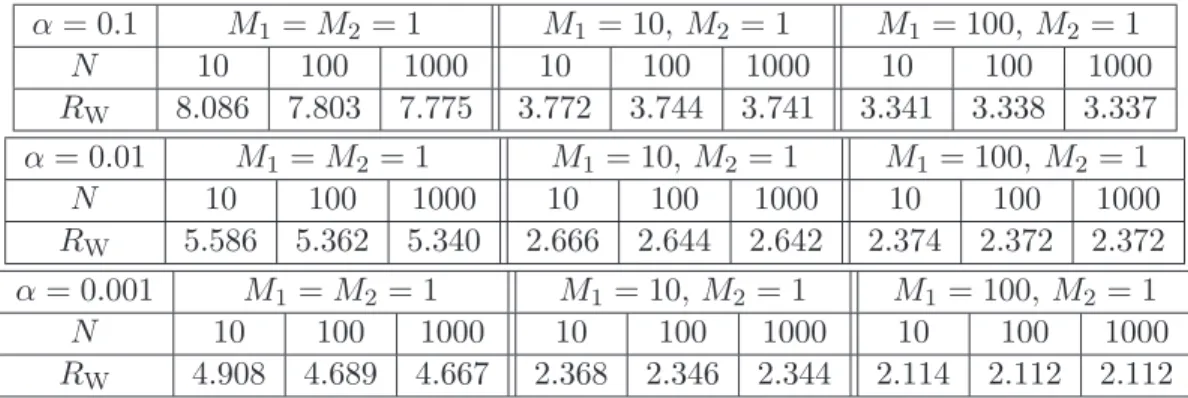
In Table 1, we provide the ratios RW of the widths of the confidence intervals, as given by Corollary 1 and their lower bounds for some combinations of risks α and parameters
α= 0.1 M1 =M2= 1 M1= 10, M2 = 1 M1 = 100, M2 = 1
N 10 100 1000 10 100 1000 10 100 1000
RW 8.086 7.803 7.775 3.772 3.744 3.741 3.341 3.338 3.337
α= 0.01 M1 =M2 = 1 M1 = 10, M2 = 1 M1= 100, M2 = 1
N 10 100 1000 10 100 1000 10 100 1000
RW 5.586 5.362 5.340 2.666 2.644 2.642 2.374 2.372 2.372
α= 0.001 M1 =M2 = 1 M1 = 10, M2 = 1 M1 = 100, M2 = 1
N 10 100 1000 10 100 1000 10 100 1000
RW 4.908 4.689 4.667 2.368 2.346 2.344 2.114 2.112 2.112
Table 1: Ratios RW of the widths of the confidence intervals as given by Corollary 1 and their lower bounds from Proposition 3.
2.2 Constrained case
Now consider a convex stochastic problem of the form
Opt = min
x∈X
f0(x) := Z
Ξ
F0(x, ξ)P(dξ) : fi(x) :=
Z
Ξ
Fi(x, ξ)P(dξ)≤0,1≤i≤m
, (9)
where, similarly to the above, X is a convex compact set in a Euclidean space E,P is a Borel probability distribution on Rk, Ξ is the support of P, and
Fi(x, ξ) :E×Ξ→R,0≤i≤m,
are Borel functions convex in x and P-summable in ξ for every x, so that the functions fi,
0≤i≤m, are convex. As in the previous section, we assume that E is equipped with a norm
k · k, the conjugate norm being k · k∗, and a compatible with k · k distance-generating function for the unit ball Bk·k of the norm.
Assuming that we can sample from the distribution P, and given a sample size N, we can build Sample Average Approximations (SAA’s) of functionsfi, 0≤i≤m:
fi,N(x, ξN) =
1
N N
X
t=1
Fi(x, ξt).
Here, as above, ξ1, ξ2, ... are drawn, independently of each other from P and ξN = (ξ1, ..., ξN).
Same as above, we want to use these SAA’s of the objective and the constraints of (9) to infer conclusions on the optimal value of the problem of interest (9).
Our first observation is that in the constrained case, one can hardly expect a reliable and tight approximation to Opt to be obtainable from noisy information. The reason is that in the general constrained case, even the special one whereFi (and thusfi) are affine inx, the optimal
value is highly unstable: arbitrarily small perturbations of the data(e.g., the coefficients of affine functions Fi in the special case or parameters of distributionP) can result in large changes in
is to impose an priori upper bound on the magnitude of optimal Lagrange multipliers for the problem of interest, e.g., by imposing the assumption that this problem is strictly feasible, with the level of strict feasibility
β:=−min
x∈Xmax[f1(x), ..., fm(x)] (10)
lower-bounded by a known in advance positive quantity. Since in many cases an priori lower bound onβ is unavailable, we intend in the sequel to utilize an alternative approach, specifically, as follows. Let us associate with (9) the univariate (max-)function
Φ(r) = min
x∈Xmax[f0(x)−r, f1(x), ..., fm(x)].
Clearly, Φ is a continuous convex nonincreasing function of r ∈ R such that Φ(r) → ∞ as
r → −∞. This function has a zero if and only if (9) is feasible, and Opt is nothing but the smallest zero of Φ.
Definition 1. Given ǫ >0, a real ρ ǫ-underestimatesOpt if ρ≤Opt and Φ(ρ)≤ǫ.
Note that Φ(ρ)≤ǫimplies that
ρ≥Opt(ǫ) := min
x∈X[f0(x)−ǫ:fi(x)≤ǫ,1≤i≤m].
Thus,ρ ǫ-underestimates Opt if and only if ρ is in-between the optimal value of the problem of interest (9) and the problem obtained from (9) by “optimistic” ǫ-perturbation of the objective and the constraints.
Remark. Let ρ ǫ-underestimate Opt. When (9) is feasible and the magnitude λ of the left derivative Φ(·) taken at Opt is positive, from convexity of Φ it follows that
Opt− ǫ
λ ≤ρ <Opt.
Thus, unlessλ is small, ρ is an O(ǫ)-tight lower bound on Opt. Note that when (9) is strictly feasible, λ indeed is positive, and it can be bounded away from zero. Indeed, we have the following
Lemma 1. Let λbe the left derivative of ΦatOpt and assume thatβ given by (10) is positive. Then
λ≥ β
V +β, V = maxx∈X f0(x)−Opt.
In respect to the constrained problem (9), our main result is as follows:
Proposition 4. Let
L(x, ξ) = max
Assume that fi, 0≤i≤m, are differentiable onX, and that for some positive M1, M2 one has
for i= 0,1, ..., m:
Ehe(Fi(x,ξ)−fi(x))2/M12 i
≤e, EheL2(x,ξ)/M22 i
≤e
for allx from an open set X+ containing X. Assume also that (9)is feasible. Assume that for N ∈Z+, s >1, and λ, µ∈[0,2√α∗N], ǫ and β satisfy
ǫ > 2N−1/2µM
1+M2RΩ2[1 +s2] +λ,
β = e−N(s2−1)
+ e−λ
2
4α∗ + (m+ 2)e− µ2
4α∗,
(11)
where Ω is given by (2), andα∗ is given in Proposition 1. Then the random quantity
OptN(ξN) = min
x∈X
h
f0,N(x, ξN)−µM1N−1/2 : fi,N(x, ξN)−µM1N−1/2 ≤0,1≤i≤m i
ǫ-underestimatesOpt with probability ≥1−β.
MinMax Stochastic Optimization. The proof of Proposition 4 also yields the following result which is of interest by its own right:
Proposition 5. In the notation and under assumptions of Proposition 4, consider the minimax problem
Opt = min
x∈Xmax[f1(x), ..., fm(x)] (12) along with its Sample Average Approximation
OptN(ξN) = min
x∈Xmax[f1,N(x, ξ
N), ..., f
m,N(x, ξN)].
Then for every N ∈Z+, s >1 andλ, µ∈[0,2√α∗N] one has
ProbnOptN(ξN)>Opt +µM1N−1/2 o
≤me−µ
2
4α∗ (13)
and
ProbOptN(ξN)<Opt−µM
1+ 2M2Ω2[1 +s2] + 2λN−1/2
≤e−µ
2
4α∗ + 2
e−N(s2−1)+ e−λ
2
4α∗
. (14)
An attractive feature of bounds (13) and (14) is that they are only weakly affected by the number mof components in the minimax problem (12).
3
Numerical experiments
3.1 Confidence intervals for problems without stochastic constraints
Here we consider three risk-averse optimization problems of the form (1) and we compare the properties of three confidence intervals for Opt computed for the confidence level 1−α= 0.9:
1. the asymptotic confidence interval
Ca(α) =
ˆ
fN(x(ξN))−qN
1−α
2 σˆN
√ N,
ˆ
fN(x(ξN)) +qN
1−α
2 σˆN
√ N
. (15)
Herex(ξN) is an optimal solution of the SAA (3) built using theN-sampleξN and qN(α) stands for theα-quantile of the standard normal distribution. The values
ˆ
fN(x(ξN)) =
1
N N
X
t=1
F(x(ξN),ξ¯t), σˆ2N =
1
N N
X
t=1
F(x(ξN),ξ¯t)2−fˆN(x(ξN))2 (16)
are computed using the second sample ¯ξN of size N independent of ξN (for a justification,
see [20]).
2. The (non-asymptotic) confidence interval CSMD(α) is built using theofflineaccuracy cer-tificates for the Stochastic Mirror Descent algorithm, cf. Section 3.2 and Theorem 2 of [9]. The non-Euclidean algorithm with entropy distance-generating function provided the best results in these experiments and was used for comparison.
3. The (non-asymptotic) confidence interval, denotedCSAA(α), is based on bounds of Propo-sition 1. Specifically, we use the lower 1−α/2-confidence boundLowSAA
of Corollary 1. To construct the upper bound we proceed as follows: first we compute the optimal solution
x(ξN) of the SAA using a simulation sampleξN of sizeN; then we compute an estimation
ˆ
f(x(ξN)) of the objective value using the independent sample ¯ξN as in (16). Finally, we build the upper confidence bound
Up′= ˆf(x(ξN)) + 2M1 r
α∗ln[4α−1]
N ,
where α∗ and M1 are as in Proposition 1 (cf. the bound (5)). Finally, the upper bound UpSAAcomputed as the minimum ofUp′ and the upper boundUpSAA
by Proposition 1, tuned for the confidence level 1−α/4, was used.1
For the sake of completeness, for three optimization problems considered in this section we provide the detail of computing of the constants involved in Appendix B. SAA formulations of these problems were solved numerically using Mosek Optimization Toolbox [1].
1It is worth to mention that in our experiments the upper bound
Sample Problem size n
size N 2 10 20 100
20 0.94 0.68 0.59 0.10
100 0.95 0.87 0.70 0.46 10 000 0.94 0.95 0.91 0.85
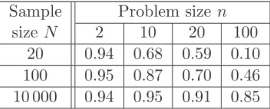
Table 2: Quadratic risk minimization. Estimated coverage probabilities of the asymptotic con-fidence intervals Ca(0.1).
3.1.1 Quadratic risk minimization
Consider the following instance of problem (1): letX be the standard simplex ofRn: X={x∈
Rn: xi ≥0,Pni=1xi = 1}, Ξ is a part of the unit box {ξ = [ξ1;...;ξn]∈Rn:kξk∞ ≤1},
F(x, ξ) =α0ξTx+
α1 2 ξ
Tx2, f(x) =α
0µTx+
α1 2 x
TV x,
withα1≥0 andµ=E{ξ},V =E{ξξT}.
In our experiments, α0= 0.1, α1 = 0.9, andξ has independent Bernoulli entries: Prob(ξi =
1) =θi, Prob(ξi =−1) = 1−θi, withθi drawn uniformly over [0,1]. This implies that
µi= 2θi−1, Vi,j =
E{ξi}E{ξj}= (2θi−1)(2θj −1) for i6=j, E{ξi2}= 1 fori=j.
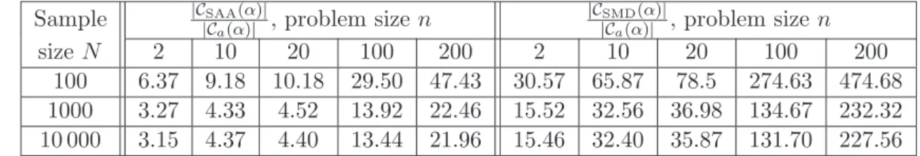
For several problem and sample sizes, we present in Table 2 the empirical “coverage probabil-ities” of the “asymptotic” confidence interval Ca(α) for α = 0.1 (“target” coverage probability 1−α= 0.9) computed over 500 realizations (the coverage probabilities of the two non-asymptotic confidence intervals are equal to one for all parameter combinations). We observe that empirical coverage probabilities degrade when the problem size nincreases (and, as expected, they tend to increase with the sample size). For instance, these probabilities are much smaller than the target coverage probability, unless the size N of the simulation sample is much larger than the problem dimension n. On the other hand, not surprisingly, the non-asymptotic bounds yield confidence intervals much larger than the asymptotic confidence interval. We report in Table 3 the mean ratio of the widths of non-asymptotic – CSAA(α) andCSMD(α) – and asymptotic con-fidence intervals Ca(α).2 These ratios increase significantly with problem size (in part because the asymptotic interval becomes indeed too short), and we observe that the confidence inter-val CSAA(α) based on Sample Average Approximation remains much smaller than the interval
CSMD(α) yielded by Stochastic Approximation. Finally, on Figure 1 we compare average over 100 problem realizations “inaccuracies” of approximate solutions delivered by SAA and SMD for “typical” problem instances of sizen= 100 for two combinations of parametersα0 and α1.
3.1.2 Markowitz portfolio optimization
We consider the instance of problem (1) where X⊂Rn is the standard simplex,ξ has normal distribution N(0,Σ) on Rn with Σi,i ≤σmax, andF(x, ξ) = α0ξTx+α1|ξTx|, with α1 ≥0, so
2Note that asymptotic estimation ˆσ
N of the noise variance often degenerates, to avoid related division by zero
Sample |CSAA(α)|
|Ca(α)| , problem sizen |C
SMD(α)|
|Ca(α)| , problem size n
size N 2 10 20 100 200 2 10 20 100 200
100 6.37 9.18 10.18 29.50 47.43 30.57 65.87 78.5 274.63 474.68 1000 3.27 4.33 4.52 13.92 22.46 15.52 32.56 36.98 134.67 232.32 10 000 3.15 4.37 4.40 13.44 21.96 15.46 32.40 35.87 131.70 227.56
Table 3: Quadratic risk minimization. Average ratio of the widths of the SAA and asymptotic confidence intervals.
101
102
103
104
105 10−6
10−5 10−4 10−3 10−2
Sample size
SAA SMD
101
102
103
104
105
106 10−10
10−9 10−8 10−7 10−6 10−5 10−4 10−3 10−2 10−1 100
Sample size
SAA SMD
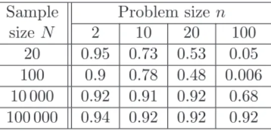
Sample Problem size n
size N 2 10 20 100
20 0.95 0.73 0.53 0.05
100 0.9 0.78 0.48 0.006
10 000 0.92 0.91 0.92 0.68 100 000 0.94 0.92 0.92 0.92
Table 4: Markowitz portfolio optimization. Estimated coverage probabilities of asymptotic confidence intervals.
Sample |CSAA(α)|
|Ca(α)| for problem sizen |C
SMD(α)|
|Ca(α)| for problem size n
size N 2 10 20 100 200 2 10 20 100 200
20 4.42 6.15 6.11 6.27 6.35 40.16 112.38 133.80 183.61 205.66
100 5.04 9.11 10.79 12.87 13.44 46.41 172.00 244.68 397.01 458.85 10 000 5.27 12.17 16.29 26.65 30.28 49.15 237.79 386.31 974.32 1088.90
Table 5: Markowitz portfolio optimization. Average ratio of the widths of the non-asymptotic and asymptotic confidence intervals.
thatf(x) =α1 p
2/π√xTΣx.
We generated instances of the problem of different size withα0 = 0.9,α1 = 0.1, and diagonal matrix Σ with diagonal entries drawn uniformly over [1,6] (σmax=
√
6).
We reproduce the experiments of the previous section in this setting, namely, for several problem and sample sizes, we compute empirical “coverage probabilities” of the confidence in-tervals over 500 realizations. We report the results for the “asymptotic” confidence intervalCa(α) in Table 4 for “target” coverage probability 1−α = 0.9 (same as above, coverage probabilities of non-asymptotic intervals are equal to one for all parameter combinations). We especially observe extremely low coverage probabilities forn= 100 andN = 20 orN = 100.
In Table 5 the average ratios of the widths of non-asymptotic and asymptotic confidence intervals are provided for the same experiment. Same as in the experiments described in the previous section, these ratios increase with problem size, and the confidence intervals by SMD are much more conservative than those by SAA.
On Figure 2 we present average over 100 problem realizations “inaccuracies” of approximate solutions delivered by SAA and SMD for “typical” problem instances of size n= 100.
3.1.3 CVaR optimization
We consider here the following CVaR optimization problem: givenε >0, find
Optε= minx′ α0E{ξTx′}+α1CVaRε(ξTx′)
x′ ∈Rn Pni=1x′i = 1, x′ ≥0, (17)
where the support Ξ ofξ is a part of the unit box{ξ = [ξ1;...;ξn]∈Rn:kξk∞≤1}, and where
CVaRε(ξTx′) = min x0∈R{
101 102 103 104 105 10−5
10−4 10−3 10−2 10−1 100
Sample size
SAA SMD
101 102 103 104 105 10−4
10−3 10−2 10−1 100
Sample size
SAA SMD
Figure 2: Markowitz portfolio optimization: empirical estimation of E{f(xN) − Opt} as
a function of N (in logarithmic scale). Left plot: simulation results for a problem with
α0 = 0.1, α1 = 0.9; right plot: results for a problem withα0= 0.9, α1 = 0.1.
is the Conditional Value-at-Risk of level 0 < ε < 1, see [17]. Observing that |ξTx′| ≤ 1 a.s., the above problem is clearly of the form (1) with X = {x = [x0;x′1;...;x′n] ∈ Rn+1 : |x0| ≤ 1, x′1, ..., x′n≥0,Pni=1x′i = 1} and
F(x, ξ) =α0ξTx′+α1
x0+ 1
ǫ[ξ
Tx′−x
0]+
.
We consider random instances of the problem with α0, α1 ∈ [0,1], and ξ with independent Bernoulli entries: Prob(ξi = 1) = θi, Prob(ξi = −1) = 1−θi, with θi, i = 1, ..., n drawn
uniformly from [0,1].
We compare the non-asymptotic confidence interval CSAA(α) for Optε to the asymptotic
confidence interval Ca(α) with confidence level 1−α = 0.9. We consider two sets of problem parameters: (α0, α1, ε) = (0.9,0.1,0.9) and the risk-averse variant (α0, α1, ε) = (0.1,0.9,0.1). The empirical coverage probabilities for the asymptotic confidence interval are reported in Table 6. As in other experiments, the coverage probability still below the target probability of 1−α= 0.9 when the sample size is not much larger than the problem size. For SAA, the coverage probabilities are equal to one for all parameter combinations.
We report in Table 7 the average ratio of the widths of non-asymptotic and asymptotic confidence intervals. Note that the Lipschitz constant of F(·, ξ) is proportional to 1/ε when
ε is small. This explains the fact that for small values of ǫ, the ratio of the widths of the proposed non-asymptotic and asymptotic confidence intervals grows up significantly, especially for problem size n+ 1 = 3.
Sample ε= 0.1, problem size n ε= 0.9, problem size n
size N 3 11 21 101 3 11 21 101
100 0.96 0.74 0.85 0.78 0.96 0.95 0.95 0.78 1000 0.95 0.88 0.86 0.67 0.95 0.92 0.84 0.84 10 000 0.92 0.93 0.91 0.94 0.92 0.95 0.96 0.96
Table 6: CVaR optimization. Estimated coverage probabilities of asymptotic confidence inter-vals.
Sample ε= 0.9, problem size n ε= 0.1, problem size n
size N 3 11 21 101 201 3 11 21 101 201
100 3.09 3.69 7.33 14.25 13.79 293.47 27.61 9.14 14.32 14.44 1000 3.25 3.67 8.63 35.04 36.72 294.16 27.04 8.72 34.43 37.42 10 000 3.22 3.68 8.61 32.08 34.00 293.92 26.91 8.66 31.70 34.18
Table 7: CVaR optimization. Average ratio |CSAA(α)|
|Ca(α)| of the widths of the non-asymptotic and
asymptotic confidence intervals.
101 102 103 104 105
10−9 10−8 10−7 10−6
10−5 10−4 10−3
10−2 10−1 100
Sample size
SAA SMD
3.2 Lower bounding the optimal value of a minimax problem
We illustrate here the application of Proposition 5 to lower bounding the optimal value of the MinMax problem (12). To this end we consider a toy problem
Opt = min
x max
"
fi(x), i= 1, ...,3, x= [u;v]v∈R, u∈Rn, n
X
i=1
ui = 1, u≥0
#
, (18)
where
f1(x) =v+E{ε−1[ξTu−v]+}+ρ1, f2(x) =E{ξTu}+ρ2, f3(x) =ρ3−E{ξTu},
εand ρ being some given parameters. The SAA of the problem reads
Opt(ξN) = min
x max
"
fi,N(x), i= 1, ...,3, x= [u;v]v∈R, u∈Rn, n
X
i=1
ui = 1, u≥0
#
, (19)
with
f1,N(x) =v+
1
N ε N
X
t=1
[ξTtu−v]+, f2,N(x) =
1
N N
X
t=1
ξtTu+ρ2, f3,N(x) =ρ3− 1
N N
X
t=1
ξTtu.
One can try to build an “asymptotic” lower bound for Opt as follows (note that here we are not concerned with theoretical validity of this construction): given the optimal solution x(ξN) to
the SAA (19), compute empirical variancesσi,N ofFi(x(ξN), ξ), then compute the lower bound
“of asymptotic risk α” according to
Opt(ξN) = max
i=1,...,3
fi,N(x(ξN))−qN
1−α
3 σi,N
√ N
.
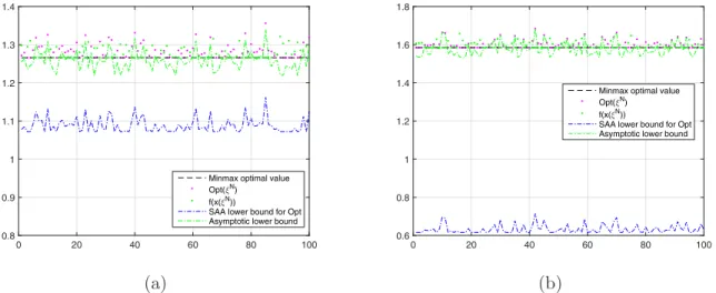
On Figure 4 we present the simulation results for the case ofξ ∈Rn with independent Bernoulli components: Prob(ξi = 1) = θi, Prob(ξi = −1) = 1−θi, with θi randomly drawn over [0,1];
parameters ρi, i = 1,2,3 are chosen in a way to ensure that f1–f3 are approximately equal at the minimizer of (18). The results of 100 simulations of the problem with n= 2 andN = 128 are presented on Figure 4 for the value of CVaR parameter ε = 0.5 and ε = 0.1. Note that in this case the risk of the lower bound Opt(ξN) is significantly larger than the prescribed risk
ε= 0.1 already for small problem dimension – the “asymptotic” lower bound failed for 33% of 7 realizations in the experiment with ε= 0.5, and for 36% of realizations in the experiment with
ε= 0.1.
3.3 Optimal value of a stochastically constrained problem
An SAA of a stochastically constrained problem, even with a single linear constraint, can easily become unstable when the constraint is “stiff”. As a simple illustration, let us consider a stochastically (linearly) constrained problem
Optρ= min "
f0(x) : f1(x)≤0, x= [u;v], v∈R, u∈Rn, n
X
ui = 1, u≥0
#
0 20 40 60 80 100 0.8
0.9 1 1.1 1.2 1.3 1.4
Minmax optimal value Opt(✂
N)
f(x(✂ N))
SAA lower bound for Opt Asymptotic lower bound
0 20 40 60 80 100
0.6 0.8 1 1.2 1.4 1.6 1.8
Minmax optimal value Opt(✂N)
f(x(✂N))
SAA lower bound for Opt Asymptotic lower bound
(a) (b)
Figure 4: Optimal value Opt of the stochastic program (18) along with lower bound derived from the results of Proposition 5 and “asymptotic” lower bound Opt(ξN). The results for ε= 0.5 on the plot (a),
forε= 0.1 on plot (b).
where
f0(x) =v+E{ε−1[ξTu−v]+}, and f1(x) =ρ−E{ξTu}, and εand ρ are problem parameters. The SAA of the problem is
Optρ(ξN) = min
x=[u;v] "
f0,N(x) : f1,N(x)≤0, v∈R, u∈Rn, n
X
i=1
ui = 1, u≥0
#
, (21)
where
f0,N(x) =v+
1
N ε N
X
t=1
[ξtTu−v]+, and f1,N(x) =ρ−
1
N N
X
t=1
ξTtu.
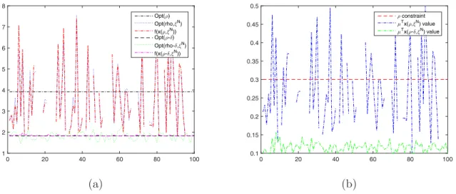
Consider now a toy example of the problem with u∈ R2, ξ ∼ N(µ,Σ) with µ = [0.1; 0.5] and Σ = diag([1; 4]). LetN = 128,ρ= 0.3, andε= 0.1. One can expect that in this case the optimal value Opt(ξN) of the SAA is unstable (in fact, the problem (21) is infeasible with probability
ProbnN1 PNt=1ξt,2 < ρ o
= Probn2N√(0,1)
N ≤ −0.2
o
= 0.128...). We compare the solution to (21) with the SAA in which the r.-h.s. ρ of the stochastic constraint is replaced with ρ−δ where
δ=qN(1−ε/n)σ√max
N 0.5815...,σmax= maxiΣi,i. On Figure 5 we present the simulation results of
0 20 40 60 80 100 1
2 3 4 5 6 7 8
Opt(✂)
Opt(rho,✄
N)
f(x(✂,✄
N))
Opt(✂-☎)
Opt(rho-☎,✄
N)
f(x(✂-☎,✄
N))
0 20 40 60 80 100
0.1 0.15 0.2 0.25 0.3 0.35 0.4 0.45 0.5
✂ constraint ➭
Tx( ✂,✄
N) value
➭ Tx(
✂-☎,✄ N) value
(a) (b)
Figure 5: Plot (a): optimal value Opt of the stochastic program (20) with constraint r.-h.s. ρand
ρ−δ, along with corresponding optimal values of the SAA. Plot (b): “true value” of the linear form
µTx(ξN) at the SAA solution.
A
Proofs
A.1 Preliminaries: Large deviations of vector-valued martingales
The result to follow is a slightly simplified and refined version of the bounds on probability of large deviations for vector-valued martingales developed in [6, 12].
Letk · kbe a norm on Euclidean spaceE,k · k∗ be the conjugate norm, andBk·k be the unit ball of the norm. Further, letω be a continuously differentiable distance-generating function for
Bk·k compatible with the normk · kand attaining its minimum onBk·k at the origin: ω′(0) = 0, withω(0) = 0 and Ω = maxx:kxk≤1
p
2[ω(x)].
Lemma 2. Let d1, d1, ...be a scalar martingale-difference such that for some σ >0 it holds
E{ed2t/σ2|d
1, ..., dt−1} ≤e a.s., t= 1,2, ...
Then
Probn XN
t=1dt | {z }
DN
> λσ√No≤
e−λ
2
4α∗, 0≤λ≤2√α ∗N ,
e−λ
2
3 , λ >2√α
∗N ,
(22)
where α∗ is defined in Proposition 1.
Proof. Assuming without loss of generality thatσ = 1 observe that under Lemma’s premise we have E{eα∗θ2d2
t|d1, ..., dt
−1} ≤ eα∗θ
2
whenever α∗θ2 ≤ 1 where α
∗ is defined in Proposition 1,
and therefore for almost alldt−1 = (d1, ..., dt−1) we have for 0≤θ≤ √1α∗
θdt t−1 α θ2d2
t−1 α θ2d2
Thus, for 0≤θ≤ √1α
∗, we have E{e
θDN} ≤eα∗θ2N, and ∀λ >0
Prob{DN > λ √
N} ≤eα∗θ2N−λθ√N.
When minimizing the resulting probability bound over 0 ≤θ ≤ √1α∗ we get the inequality (22) forλ∈[0,2√α∗N]: Prob{DN > λ
√
N} ≤e−λ
2
4α∗. The corresponding bound forλ >2√α ∗N
is given by exactly the same reasoning as above in which (23) is substituted with the inequality
Eneθdtdt−1o≤E
e3θ
2 8 +
2d2t
3 dt−1
≤e3θ
2 8 +
2 3 ≤e
3θ2
4
when θ >1/√α∗.
Proposition 6. Let (χt)t=1,2,..., χt∈E, be a martingale-difference such that for some σ >0 it holds
Enekχtk2∗/σ2χ1, ..., χt−1
o
≤e a.s., t= 1,2, ... (24)
Then for every s >1, we have
Prob ( k N X t=1
χtk∗ > σ
" Ω√N
2 [1 +s
2] +λ√N #)
≤
e−N(s2−1)
+ e−λ
2
4α∗, 0≤λ≤2√α∗N,
e−N(s2−1)
+ e−λ
2
3 , λ >2√α
∗N ,
(25)
where α∗ is defined in Proposition 1 and Ω is given by (2).
Proof. By homogeneity, it suffices to consider the case whenσ = 1, which we assume from now on.
10. Let γ >0. We denote
Vx(u) =ω(u)−ω(x)− hω′(x), u−xi [u, x∈Bk·k]
and consider the recurrence
x1 = 0, xt+1 = argmin
y∈Bk·k
[Vxt(y)− hγχ, yi].
Observe that xt is a deterministic function of χt−1 = (χ1, ..., χt−1), and that by the standard properties of proximal mapping (see. e.g. [12, Lemma 2.1]),
∀(u∈Bk·k) :γ N
X
t=1
hχt, u−xti ≤V0(u)−VxN+1(u) +
γ2
2
N
X
t=1
kχtk2∗≤ 1
2Ω
2+γ2 2
N
X
t=1
kχtk2∗.
Thus
max
u∈Bk·k
DXN
t=1
χt, u
E
≤ Ω
2
2γ + γ
2
N
X
t=1
kχtk2∗
| {z }
ηN
+
N
X
t=1
hχt, xti
| {z }
Settingγ = Ω/√N, we arrive at
max
u∈Bk·k
DXN
t=1
χt, u
E
≤ Ω √
N
2 h
1 +ηN
N
i
+ζN. (26)
Invoking (24), we get
E{eηN} ≤eN
(recall thatσ = 1), whence
∀s >0 : ProbηN > s2N ≤min
h
1,eN(1−s2)i. (27)
20. When invoking (24) and taking into account that xt is a deterministic function of χt−1
such thatkxtk ≤1 (since xt∈Bk·k), we get
E{hχt, xti|χt−1}= 0, E{ehχt,xti
2
|χt−1} ≤e (28) Applying Lemma 2 to the random sequence dt =hχt, xti,t= 1,2, ... (which is legitimate, with σ set to 1, by (28)), we get
ProbnζN > λ √
No≤
e−λ
2
4α∗, 0≤λ≤2√α ∗N ,
e−λ
2
3 , λ >2√α
∗N .
(29)
In view of (27) and (29), relation (26) implies the bound (25) of the proposition.
A.2 Proof of Proposition 1
Letx∗ be an optimal solution to (SP), and let h=∇f(x∗), so that by optimality conditions
hh, x−x∗i ≥0 ∀x∈X. (30)
10. Setting δ(ξ) = F(x∗, ξ) −f(x∗), invoking (4.a) and applying Lemma 2 to the random sequence dt=δ(ξt) and σ=M1 (which is legitimate by (4.a)), we get
∀(N ∈Z+, µ∈[0,2 p
α∗N]) : Probn1
N N
X
t=1
δ(ξt)> µM1N−1/2 o
≤e−µ
2
4α∗. (31)
Since clearly
OptN(ξN)≤fN(x∗, ξN) = Opt +
1
N N
X
t=1
δ(ξt),
we get
ProbnOptN(ξN)>Opt +µM1N−1/2 o
≤e−µ
2
20. It is immediately seen that under the premise of Proposition 1, for every measurable vector-valued functiong(ξ)∈∂xF(x∗, ξ) we have
h= Z
Ξ
g(ξ)P(dξ). (33)
Observe that hN(ξN) = N1 PNt=1g(ξt) is a subgradient of fN(x, ξN) at the point x∗.
Conse-quently, for all x∈X,
fN(x, ξN)≥fN(x∗, ξN) +hhN(ξN), x−x∗i ≥ [f(x∗) +hh, x−x∗i]
| {z }
≥Opt by (30)
+[[fN(x∗, ξN)−f(x∗)] +hhN(ξN)−h, x−x∗i]
≥ Opt + 1
N N
X
t=1
δ(ξt)− kh−hN(ξN)k∗kx−x∗k ≥Opt +
1
N N
X
t=1
δ(ξt)−2kh−hN(ξN)k∗R
(the concluding inequality is due to x, x∗ ∈ X and thus kx−x∗k ≤2R by definition of R). It follows that
OptN(ξN)≥Opt + 1
N N
X
t=1
δ(ξt)−2kh−hN(ξN)k∗R. (34)
Applying Lemma 2 to the random sequence dt=−δ(ξt) we, similarly to the above, get
∀(N, µ∈[0,2pα∗N]) : Prob (
1
N N
X
t=1
δ(ξt)<−µM1N−1/2 )
≤e−µ
2
4α∗. (35)
Further, setting ∆(ξ) =g(ξ)− ∇f(x∗), the random vectorsχt= ∆(ξt),t= 1,2, ..., are i.i.d.,
zero mean (by (33)), and satisfy the relation
Enekχtk2∗/M22 o
≤e
by (4.b); besides this,hN(ξN)−h= N1 PNt=1χt. Applying Proposition 6, we get
∀(N ∈Z+, s >1, λ∈[0,2√α∗N]) :
Prob{kh−hN(ξN)k∗ ≥M2Ω2[1 +s2] +λN−1/2} ≤e−N(s
2−1)
+ e−λ
2
4α∗.
This combines with (34), and (35) to imply (6).
A.3 Proof of Proposition 2
Due to similarity reasons, it suffices to prove the proposition forL=R= 1. LetB2 be the unit Euclidean ball of Rn, and let for a unit v ∈Rn and 0< θ ≤π/2, hv,θ be the spherical cap of B2 with “center” v and angle θ. In other words, ifδ = 2 sin2(θ/2) is the “elevation” of the cap
angle between every two distinct vectors of the system is >2θ, so that the spherical caps hv,θ
with v ∈ Dθ are mutually disjoint, while the spherical caps hv,ϑ cover Sn−1. If we denote
An−1(ϑ) the area of the spherical cap of angle ϑ ≤ π/2, then Card(Dθ)An−1(ϑ) ≥ sn−1(1), where sn−1(r) = 2π
n/2rn−1
Γ(n/2) is the area of the n-dimensional sphere of radius r. Note that
An−1(ϑ) satisfies
An−1(ϑ) = Z ϑ
0
sn−2(sint)dt=sn−2(1) Z ϑ
0
sinn−2tdt≤sn−2(1) Z ϑ
0
tn−2dt=sn−2(1)
ϑn−1
n−1.
We conclude that
Card(Dθ)≥
sn−1(1)(n−1)
sn−2(1)ϑn−1 ≥ 3ϑ1−n
for n ≥ 2. From now on we fix θ = 1/8 and when choosing ϑ arbitrarily close to 4θ = 1
2, we
conclude that for any n≥2 one can build Dθ such that Card(Dθ)≥2n.
Now consider the following construction: for v ∈ Dθ, let gv,θ(·) : B2 → R be defined according to gv,θ(x) = [vTx−(1−δ)]+, whereδ = 2 sin2(θ/2) = 0.0078023... is the elevation of hv,θ. Let us put
f(x) = X
v∈Dθ
gv,θ(x),
and consider the optimization problem Opt = min[f(x) : x ∈ B2]. Since gv,δ is affine on hv,δ
and vanishes elsewhere onB2, and kvk2 = 1, we conclude thatf is Lipschitz continuous on B2 with Lipschitz constant 1. Let now
F(x, ξ) = X
v∈Dθ
2ξvgv,θ(x),
whereξv, v∈Dθ are i.i.d. Bernoulli random variables with Prob{ξv = 0}= Prob{ξv = 1}= 12.
Note that Eξ{F(x, ξ)}=f(x)∀x∈B2. Further, for x∈hv,θ,Eξ{F(x, ξ)2−f(x)2}=g2v,θ(x)≤ δ2,and
kF′(x, ξ)−f′(x)k22=k(2ξv −1)g′v,θ(x)k22 ≤1. Let us now consider the SAAfN(x) of f,
fN(x) =
1
N N
X
t=1
F(x, ξt) =
X
v∈Dθ
1
N N
X
t=1
ξt,vgv,θ(x)
| {z }
gN v,θ(x)
, (36)
ξt, t= 1, ..., N being independent realizations of ξ, and the problem of computing
Opt(ξN) = min[fN(x) : x∈B2]. (37)
Note that for a given v ∈Dθ, Prob{PNt=1ξt,v = 0}= 2−N. Due to the independence of ξv, we
have
Prob ( N
X
ξt,v >0, ∀v∈Dθ
)
= (1−2−N)Card(Dθ)≤(1−2−N)2n ≤e−
2n
forN ≤n. We conclude that forN ≤n, with probability≥1−e−1, at least one of the summands in the right-hand side of (36), let it be gN
¯
v,θ(x), is identically zero on B2. The optimal value
Opt(ξN) of (37) being zero, the point x(ξN) = ¯v is clearly a minimizer of f
N(x) on B2, yet
f(x(ξN)) =δ, i.e., (7) holds with c0=δ.
A.4 Proof of Proposition 3
10. Let us consider a family of stochastic optimization problems as follows. Let k · k=k · k2 and let X be the unitk · k2-ball in Rn. Given a unit vector✚✚g, h inRn, positive reals σ, s and δ, d, and setting ξ = [η;ζ]∼ N(0, I2), consider two integrants:
F0(x, ξ) =σηhTx+sζ, F1(x, ξ) = (δh+σηh)Tx+ (sζ−d),
so that
f0(x) :=Eξ{F0(x, ξ)}= 0, f1(x) :=Eξ{F1(x, ξ)}=δhTx−d.
Let us now check that F0 and F1 verify the premises of Proposition 1. In the notation of Proposition 1, we have forF1
L(x, ξ) =k[δh+σηh]−δhk2 =σ|η|,
whence, setting M2 =σ/γ with γ2 = 12(1−e−2),
Eξexp{L(x, ξ)2/M22} = exp{1}.
Similarly, setting M1 =
√
σ2+s2/γ, we have
Eξexp{(ση+sζ)2/M12} = exp{1},
so that, for everyz∈[−1,1],
Eξexp{(σηz+sζ)2/M12} ≤exp{1}.
When x∈Rn and kxk2≤1, we have F1(x, ξ)−f1(x) =σηhTx+sζ, therefore
Eξ
exp{(F1(x, ξ)−f1(x))2/M12} ≤exp{1}.
We conclude that F =F1 satisfies the premise of Proposition 1 with
M1 = p
σ2+s2/γ, M
2 =σ/γ.
20. Now, with X ={x ∈ Rn : kxk2 ≤ 1}, the optimal values in the problems of minimizing over X the functions f0 andf1 are, respectively,
Opt0 = 0, Opt1 =−δ−d.
Suppose that there exists a procedure which, under the premise of Proposition 1 with some fixedM1,M2, is able, givenN observations of∇xF(·, ξt), F(·, ξt), to cover Opt, with confidence
1−α, by an interval of width W. Note that when W < |Opt1|, the same procedure can distinguish between the hypotheses stating that the observed first order information onf comes from F0 or fromF1, with risk (the maximal probability of rejecting the true hypothesis)α. On the other hand, when F = F0 or F = F1, our observations are deterministic functions of the
samples ω1,...,ωN drawn from the 2-dimensional normal distribution N
0 0
,
σ2 0 0 s2
for F =F0, and N
δ d
,
σ2 0 0 s2
for F =F1. It is well known that deciding between
such hypotheses with risk≤α is possible only if r
δ2
σ2 +
d2
s2 ≥ 2
√
NErfinv(α).
We arrive at the following lower bound on W, givenM1,M2, with M1 ≥M2 >0:
W ≥ max
δ≥0, d≥0 (
δ+d: s
δ2
γ2M2 2
+ d2
γ2(M2
1 −M22)
≤ √2
NErfinv(α)
)
= 2√γM1
N Erfinv(α) = W.
A.5 Proof of Lemma 1
Without loss of generality we may assume that Opt = 0. Let ¯x be such that fi(¯x) ≤ −β,
1≤i≤m. Given δ >0, there exists xδ∈X such thatf0(xδ) +δ ≤Φ(−δ) andfi(xδ)≤Φ(−δ),
1≤i≤m; note that Φ(−δ)>0 due to−δ <0 = Opt. The point
x= Φ(−δ)
β+ Φ(−δ)x¯+
β
β+ Φ(−δ)xδ
belongs to X and is feasible for (9), since fori≥1 one has
fi(x)≤
Φ(−δ)
β+ Φ(−δ)fi(¯x) +
β
β+ Φ(−δ)fi(xδ)≤ −
Φ(−δ)β β+ Φ(−δ) +
βΦ(−δ)
β+ Φ(−δ) = 0.
As a result,
0 = Opt≤f0(x)≤
Φ(−δ)
β+ Φ(−δ)f0(¯x) +
β
β+ Φ(−δ)f0(xδ)≤
Φ(−δ)V β+ Φ(−δ)+
β
β+ Φ(−δ)[Φ(−δ)−δ].
The resulting inequality implies (Φ(−δ)−Φ(0))/δ = Φ(−δ)/δ ≥ β/(β+V); when passing to
A.6 Proof of Proposition 4
Let us fix parameters N,s,λ,µ satisfying the premise of the proposition, letǫ,δ be associated with these parameters according to (11). We denote
¯
f0,N(x, ξN) =f0,N(x, ξN)−µM1N−1/2, ¯
fi,N(x, ξN) =fi,N(x, ξN)−µM1N−1/2, 1≤i≤m, and set
ΦN(r, ξN) = min x∈Xmax
¯
f0,N(x, ξN)−r,f¯1,N(x, ξN), ...,f¯m,N(x, ξN)
.
Then ΦN(r, ξN) is a convex nonincreasing function ofr ∈R such that
OptN(ξN) = min{r: ΦN(r, ξN)≤0}.
Finally, let ¯r be the smallest r such that Φ(r) ≤ ǫ. Since (9) is feasible and Φ(r) → ∞ as
r → −∞, ¯r is a well defined real which is < Opt (since Opt is the smallest root of Φ) and satisfies Φ(¯r) =ǫ.
Let us set
b
Ξ =ξN : ΦN(Opt, ξN)≤0
| {z }
Ξ1
∩ξN : ΦN(¯r, ξN)>0
| {z }
Ξ2
.
Since ΦN(r, ξN) is a nonincreasing function ofrand OptN(ξN) is the smallest root of ΦN(·, ξN),
forξN ∈Ξ we have ¯b r ≤Opt
N(ξN)≤Opt. The left inequality here implies that Φ(OptN(ξN))≤ǫ
(recall that Φ is nonincreasing and Φ(¯r) =ǫ). The bottom line is that when ξN ∈Ξ, Optb N(ξN)
ǫ-underestimates Opt. Consequently, all we need to prove is that ξN 6∈ Ξ with probability atb mostδ.
10. Let x∗ be an optimal solution to (9). Same as in the proof of Proposition 1, for every i, 0≤1≤m, we have (see (31))
Probfi,N(x∗, ξN)> fi(x∗) +µM1N−1/2 ≤e−
µ2
4α∗,
whence for the event
Ξ′ =ξN :fi,N(x∗, ξN)≤fi(x∗) +µM1N−1/2, 0≤i≤m it holds
ProbξN 6∈Ξ′ ≤(m+ 1)e−µ
2
4α∗. (38)
By the origin of x∗ we have f0(x∗)≤Opt and fi(x∗)≤0, 1≤i≤m. Therefore, forξN ∈Ξ′ it
holds ¯f0,N(x∗, ξN)≤Opt and ¯fi,N(x∗, ξN)≤0, 1≤i≤m, that is,
ΦN(Opt, ξN)≤max[ ¯f0,N(x∗, ξN)−Opt,f¯1,N(x∗, ξN), ...,f¯m,N(x∗, ξN)]≤0,
implying thatξN ∈Ξ1. We conclude that Ξ′ ⊂Ξ1, and, by (38),
Prob{ξN 6∈Ξ1} ≤(m+ 1)e−µ
2
20. We have ǫ = Φ(¯r) = minx∈Xmax[f0(x)−r, f¯ 1(x), ..., fm(x)], whence by von Neumann’s
Lemma there exist nonnegative λi ≥0, 0≤i≤m, summing up to 1, such that
ǫ = minx∈X[ℓ(x) :=λ0(f0(x)−r¯) +Pmi=1λifi(x)]
= minx∈Xh RΞλ0[F0(x, ξ)−r¯] +
Xm
i=1λiFi(x, ξ)
| {z }
L(x,ξ)
P(dξ)i.
Under the premise of the proposition, the integrand F satisfies all assumptions of Proposition 1. Setting
ℓN(x, ξN) =
1
N N
X
i=1
L(x, ξi)
and applying Proposition 1 we get
Prob ξ
N : min
x∈XℓN(x, ξN)<minx∈Xℓ(x)
| {z }
=ǫ
−µM1+Ω[1 +s2] + 2λM2RN−1/2
≤e−N(s2−1)
+ e−µ
2
4α∗ + e− λ2
4α∗.
Now, in view of
ℓN(x, ξN) =λ0[ ¯f0,N(x, ξN)−r¯] + m
X
i=1
λif¯i,N(x, ξN)
| {z }
¯
ℓN(x,ξN)
+µM1N−1/2,
and due to the evident relation minx∈Xℓ¯N(x, ξN)≤ΦN(¯r, ξN), we get
ProbnΦN(¯r, ξN)< ǫ−µM1+Ω[1 +s2] + 2λM2RN−1/2−µM1N−1/2 o
≤ Prob
min
x∈XℓN(x, ξ
N)< ǫ−2N−1/2µM
1+M2R
Ω 2[1 +s
2] +λ
≤ e−µ
2
4α∗ + e−N(s2−1)+ e−λ
2
4α∗.
By (11), we have
ǫ−2
µM1+M2R
Ω 2[1 +s
2] +λ
N−1/2 >0,
and we arrive at
ProbξN 6∈Ξ2 = ProbΦN(¯r, ξN)≤0 ≤e− µ2
4α∗ + e−N(s
2
−1)+ e−λ2
4α∗.
The latter bound combines with (39) to imply the desired relation
ProbξN 6∈Ξ ≤e−µ
2
4α∗ + e−N(s2−1)+ e−λ
2
4α∗ + (m+ 1)e− µ2
B
Evaluating approximation parameters
For the sake of completeness we provide here the straightforward derivations of the parameter estimates used to build the bounds in the numerical section.
B.1 Notation
Let P be a Borel probability distribution on Rk and let Ξ be the support of P. Consider the space C of all Borel functions g(·) : Ξ → R such that Eξ∼P{exp{g2(ξ)/M2}} < ∞ for some M =M(g). For g∈ C, we set
π[g] = infM ≥0 : Eξ∼P{exp{g2(ξ)/M2}} ≤exp{1} . (40)
It is well known thatC is a linear subspace in the space of real-valued Borel functions on Ξ and
π[·] is a semi-norm on this (Orlicz) space. Besides, for a constant g(·) ≡a we have π[g] =|a|, and |g(·)| ≤ |h(·)| withh∈ C and Borel gimplies g∈ C and π[g]≤π[h].
Given a convex compact set X ⊂Rn, a normk · k on Rn, and a continuously differentiable distance-generating functionω(·) for the unit ballBk·k which is compatible with this norm, letR
be the radius of the smallestk·k-ball containingX. Given a Borel functionF(x, ξ) :Rn×Ξ→R
which is convex in x∈Rn and P-summable in ξ for every x, let
f(x) =E{F(x, ξ)}: X→R.
We set
M1,∞ = supx∈X,ξ∈Ξ|F(x, ξ)−f(x)|,
M1,exp = supx∈Xπ[F(x,·)−f(x)], L(x, ξ) = supg∈∂xF(x,ξ),h∈∂f(x)kg−hk∗,
M2 = supx∈Xπ[L(x,·)].
Note that adding to F(x, ξ) a differentiable function g of x: F(x, ξ) 7→F(x, ξ) +g(x) does not affect the quantities M1,∞,M1,exp, and M2.
Our goal is to compute upper bounds on M1,∞, M1,exp, and M2 in the different settings of Section 3.1.1.
B.2 Quadratic risk minimization
In this case
• X={x= [x1;...;xn]∈Rn :x1, ..., xn ≥0,Pni=1xi = 1}, • Ξ is a part of the unit box {ξ= [ξ1;...;ξn]∈Rn:kξk∞≤1},
• F(x, ξ) = α0ξTx+ α21 ξTx2, with α1 ≥ 0, and f(x) = α0µTx+ α21xTE{ξξT}x, where
µ=E{ξ}.
The parametersM1,M2,R and Ω of construction can be set according to:
M1 ≤2|α0|+
α1
2 , M2 = 2|α0|+α1, R= 1, Ω =
1, n= 1
√
2, n= 2
ln(n)q1+ln(2en), n≥3.
Indeed, forξ∈Ξ andx∈X, we get
|F(x, ξ)−f(x)| ≤ |α0||(ξ−µ)Tx|+ α1
2 |x
T(V
−ξξT)x| ≤ |α0|kξ−µk∞+ α1
2 kV −ξξ
T k∞.
SinceV is positive semidefinite withkVk∞≤1, andkξk∞≤1, we have|xT(V
−ξξT)x | ≤1, and
M1,exp≤M1,∞≤ |α0|(1 +kµk∞) + α1
2 ≤2|α0|+
α1
2 .
Further, let us equipRn with the normk · k=k · k1, so thatk · k∗=k · k∞, and endow the
unit ball of the norm with the distance generating function3
ω(x) = 1
pγ n
X
i=1
|xi|p, p=
2 forn≤2,
1 + 1/ln(n) forn≥3, , γ=
1, n≤1
1
2, n= 2,
1
e ln(n), n≥3
(42)
resulting in Ω =qpγ2 and R= 1. Now letx∈X andξ∈Ξ, and letg be a subgradient ofF(x, ξ) with respect tox, and hbe a subgradient off atx. We have
g=α0ξ+α1ξ(ξTx), h=α0µ+α1V x,
thus
kg−hk∗≤ |α0|kξ−µk∞+α1kV −ξξ ⊤
k∞≤ |α0|(1 +kµk∞) +α1.
We conclude that
M2≤ |α0|(1 +kµk∞) +α1≤2|α0|+α1.
B.3 Markowitz portfolio optimization
Here the situation is as follows:
• X={x= [x1;...;xn]∈Rn :x1, ..., xn ≥0,Pni=1xi = 1},
• ξ∼ N(0,Σ) on Rn, Σ≻0,
• F(x, ξ) =α0ξTx+α1|ξTx|, with α1 ≥0.
We have f(x) = q2πα1σx, with σx = √
xTΣx. In this case one can set Ω and R as in (41),
along with
M1 = hq
2e2
e2−1|α0|+
√
2α1 i
σmax,
M2 = (|α0|+α1)σmax p
2(2 + lnn) +α1σmax q
2
π,
whereσ2max= max1≤i≤nΣi,i.
Indeed, we haveξTx
∼ N(0, σ2
x), we conclude thatf(x) =α1
q
2
πσx,whence
|F(x, ξ)−f(x)| ≤ |α0||ξTx|+α1||ξTx| −
p
2/πσx|=σxh|α0||ηx|+α1||ηx| −
p 2/π|i
whereηx=ξTx/σx
∼ N(0,1). By direct computation we get
π[|ηx|] =ν:= r
2e2
e2−1 = 1.52...
Next, settingκ=p2/πwe observe that
1 √
2π
R
exp{||s| −κ|2/2 −s2/2
}ds=κR0∞exp{[s2
−2κs+κ2
−s2]/2 }ds
=κR0∞exp{κ2/2
−κs}ds= exp{κ2/2
}<exp{1},
implying that
π[||ηx| −p2/π|]≤√2.
As a result,
π[F(x,·)−f(x)]≤σxh|α0|π[|ηx|] +α1π[||ηx| −
p
2/π|]i≤σxhν|α0|+ √
2α1
i
.
Taking into account that for allx∈X σ2
x=xTΣx≤ kΣk∞, we arrive at
M1,exp≤
h
ν|α0|+ √
2α1
i p
kΣk∞=
h
ν|α0|+ √
2α1
i
σmax. (43)
Letx∈X, and letgbe a subgradient with respect toxofF(x, ξ), andhbe a subgradient off(x). We have
g=α0ξ+α1ξχ
withχ=χ(x, ξ)∈[−1,1], so that
kgk∞≤[|α0|+α1]kξk∞.
Note that
∂h√xTΣxi=
( n
xTΣx−1/2Σxo, x
6
= 0,
Σ1/2u,
kuk2≤1 , x= 0.
Therefore, for allh∈∂f(x) one has
khk∞≤α1
r 2
πsupx6=0
kΣxk∞ √
xTΣx =α1
r 2
πsupy6=0 kΣ1/2y
k∞ kyk2
=α1
r 2
πkΣ 1/2
k2,∞≤α1σmax
r 2
π,
and
kg−hk∗=kg−hk∞≤[|α0|+α1]kξk∞+α1σmax
r 2
π,
that is,
L(x, ξ)≤[|α0|+α1]kξk∞+α1σmax
r 2
π.
We conclude that
π[L(x,·)]≤[|α0|+α1]π[kξk∞] +α1σmax
r 2
We now use the following simple result.4
Lemma 3. Letξbe a zero-mean Gaussian random vector inRn, and letσ¯2≥max
1≤i≤nE{ξi2}.
Then for M ≥σ¯p2(2 + lnn)
Eekξk2∞/M 2
≤e.
Proof. Letηn= max1≤i≤n|ξi|. We have the following well-known fact:
ψn(r) := Prob{ηn ≥r} ≤minn1, ne−r
2
2 ¯σ2
o
.
Therefore, for|t|<(√2¯σ)−1,
Eet2η2n = −
Z ∞
0
et2r2dψn(r) = 1 + Z ∞
0
2t2ret2r2ψn(r)dr
≤ e2t2σ¯2lnn+ 2nt2
Z ∞
¯ σ√2 lnn
rexpn−(1−2t 2σ¯2)r2
2¯σ2
o
dr
= e2t2σ¯2lnn+ 2t
2σ¯2
1−2t2¯σ2e 2t2
¯ σ2
lnn = n2t
2 ¯ σ2
1−2t2¯σ2.
Note that e−x≤1−x/2 for 0≤x≤1. Thus for alln≥1 andt≤ σ¯p2(2 + lnn)−1,
n2t2 ¯ σ2
1−2t2σ¯2 ≤
e2+lnlnnn
1− 1 2+lnn
= e1−2+ln2 n2 + lnn
1 + lnn ≤e.
Finally, using the result of the lemma we conclude from (44) that one can take for M2
the expression
(|α0|+α1)σmax
p
2(2 + lnn) +α1σmax
r 2
π. (46)
B.4 CVaR optimization
Consider the portfolio problem of Section 3.1.3. With some terminology abuse, in what follows, we refer to the special case n= 1 with x1 ≡1 as to the case ofn= 0.
• X={x= [x0;x1;...;xn]∈Rn+1 : |x0| ≤1, x1, ..., xn ≥0,Pni=1xi= 1},
• Ξ be a part of the unit box{ξ = [ξ1;...;ξn]∈Rn:kξk∞≤1},
4In fact, in the numerical experiments we have used a slightly better boundM
2which can be defined as follows.
Lettn, 0< tn< σmax be the unique solution of the equation
˜
hn(tn) =
n2t2 nσ
2 max
1−2t2
nσ2max = e
(observe that ˜hn(·) is monotone on ]0,√2σ1
max[, sotn can be computed using bisection). The same reasoning as in the proof of Lemma 3 results in the bound
M2=
(|α0|+α1)
tn
+α1σmax
r
2
π. (45)
For instance, in the experiments of Section 3.1.2, forσmax=
√