arXiv:0806.4659v1 [math.DG] 28 Jun 2008
Lower bounds for index of Wente tori
Levi Lopes de Lima, Vicente Francisco de Sousa Neto and Wayne Rossman
Dedicated to Katsuhiro Shiohama on the occasion of his sixtieth birthday.
Abstract
We show numerically that any of the constant mean curvature tori first found by Wente must have index at least eight.12
1
Introduction
The Hopf conjecture asked if all closed surfaces immersed inR3 with constant mean curvature
H must be round spheres. It was proven true when either the surface has genus zero by Hopf himself [H], or the immersion is actually an embedding by Alexandrov [H]. However, it does not hold in general, and the first counterexamples, of genus 1, were found by Wente [We]. Abresch [A] and Walter [Wa] made more explicit descriptions for these surfaces of Wente, which all have one family of planar curvature lines [Sp]. We call these surfaces the original Wente tori.
Constant mean curvature surfaces are critical for area, but not necessarily area mini-mizing, for all compactly supported volume-preserving variations. Hence the index – loosely speaking, the dimensionof area-reducing volume-preserving variations, to be defined in Sec-tion 3 – can be positive. If it is zero, the surface is stable. Do Carmo and Peng [CP] showed that the only complete stable minimal surface is a plane. Fischer-Colbrie [FC] showed that a complete minimal surface in R3 has finite index if and only if it has finite total curvature,
and that the catenoid and Enneper’s surface have index 1. Likewise, for surfaces with con-stant mean curvature H 6= 0, Barbosa and Do Carmo [BC] showed that only round spheres are stable, and Lopez and Ros [LR] and Silveira [Si] independently showed that they have finite index if and only if they are compact. This leaves open the question of whether there exist surfaces with constant mean curvature H 6= 0 and low positive index, for example with index 1.
The third author [R1], [R2] showed numerically that the most natural candidates for unstable surfaces of constant mean curvature H 6= 0 with low index – the original Wente tori – all have index at least 7, and with a numerical experiment suggested that the sharpest lower bound is either 8, 9, or 10, and is most likely 9. This leads one to conjecture that all closed surface with constant mean curvature H 6= 0 have index at least 9.
The purpose of this article is to show that the original Wente tori all have index at least 8, improving the lower bound of [R1], [R2]. The final part of our argument relies on numerics.
2
The original Wente tori
In this section we shall give a brief description of the original Wente tori, based on [Wa]. Later, we shall assume that the mean curvature H is 1/2, but in this and the next section we shall only assume that H is a nonzero constant.
Let X− : C/Γ −→ R3 be a conformal immersion of class C∞ where C/Γ is a compact
2-dimensional torus determined by the 2-dimensional lattice Γ. Note that (x, y) are then isothermal coordinates on C/Γ. The fundamental forms and the Gauss and mean curvature
functions are
I =E(dx2+dy2), II =Ldx2+ 2Mdx dy+Ndy2, K = LNE−2M2, H =
L+N
2E .
Since H is constant, the Hopf differential Φdz2 is holomorphic, where Φ = 1
2(L−N)−iM
and z =x+iy. Thus Φ is constant and X−has no umbilics points. Moreover, by a change of the coordinates (x, y), we may assume Φ = 1 and so M = 0, L =eF + 1, N = eF −1, and
(x, y) become curvature line parameters, where F :C/Γ−→R is defined by HE =eF. We
have the equations of Gauss and Weingarten:
X−xx =
1
2FxX−x− 1
2FyX−y −(e
F + 1)
N , X−yy =−
1
2FxX−x+ 1
2FyX−y −(e
F
−1)N ,
X−xy =
1
2FyX−x+ 1
2FxX−y , Nx =H(1 +e
−F)
X−x , Ny =H(1−e−F)X−y
(1)
∆F + 4H sinh F = 0,
(2)
where ∆ = ∂x∂22 +
∂2
∂y2 and N : C/Γ −→ R3 is the unit normal vector field, i.e. the Gauss
map. Therefore the problem of finding constant mean curvature immersed tori inR3 reduces
to solving the PDE system (1) and (2) by real analytic functions F,N,X−defined onR2 and
doubly periodic with respect to some fundamental lattice Γ⊂R2.
In the case of the original Wente tori, in Walter’s notation, the solutionF of (2) is:
tanh
F
4
=γ·γ·cnk(αx)cnk(αy) ,
(3)
where cnk denotes the Jacobi amplitudinus cosinus function with modulus k, and k =
sin θ, k = sin θ, forθ, θ ∈(0, π/2) and θ+θ < π/2, and
γ =√tan θ,γ =√tan θ,α =q4H sin 2θ
sin 2(θ+θ), α= q
4H sin 2θ
sin 2(θ+θ) .
Lemma 1 ([A], [Wa]). The set of all original Wente tori are in a one-to-one correspondence with the set of reduced fractions ℓ/n∈(1,2).
For eachℓ/n, we call the corresponding Wente torusWℓ/n. Following Walter’s notation,
each Wℓ/n has either one or two planar geodesic loops in the central symmetry plane: two
loops if ℓ is odd, and one loop if ℓ is even. Each loop can be partitioned into 2n congruent curve segments, and ℓ is the total winding order of the Gauss map along each loop.
The conditions for double periodicity of the position vector function X− are expressed in terms of θ and θ. Walter determined that there is exactly one
that solves one period problem. The other period problem is solved with the correct choice of θ∈(0, (π/2)−θ), and, for anyℓ/n∈(1,2), this correct choice is the unique solutionθ of
Z π/2 0
1 + tanθ tanθ cos2ϕ
1−tanθ tanθ cos2ϕ
dϕ p
1−sin2θ sin2ϕ = ℓ n
π
2
s
sin 2θ
sin 2(θ+θ) . (4)
For any ℓ/n6∈ (1,2), there is no solution θ ∈(0,(π/2)−θ) of (4). In Table 2 we give some values of θ with respect to ℓ/n.
Now, ifxℓn(resp. yℓn) denotes the length of the period ofcnk(αx) (resp. cnk(αy)), then
we have the following lemma:
Lemma 2 ([Wa]). X− : C/Γ −→ Wℓ/n ⊂ R3 is a conformal immersion (W
ℓ/n denotes the
image of X−), where
Γ =spanZ{(nxℓn,0),(0, yℓn)} whenℓ is odd, and
Γ =spanZ
nnx
ℓn
2 ,
yℓn
2
,(0, yℓn)
o
whenℓ is even.
The curves {[x0, y]|x0=constant} are mapped by X−to planar curvature lines of Wℓ/n.
The lengthsxℓn and yℓn can be computed as follows:
xℓn =
4
α Z π/2
0
dϕ p
1−k2sin2ϕ , yℓn =
4
α Z π/2
0
dϕ q
1−k2sin2ϕ .
(5)
3
The definition of index and preliminary results
The Jacobi operator associated toWℓ/n is−∆I−|II|2 onC/Γ, with|II|2 =E−2(L2+ 2M2+
N2) = 2H2(1 +e−2F) and ∆
I the Laplace-Beltrami operator associated to the metricI. The
corresponding quadratic form is
Q(u, u) =
Z
C/Γ
uL(u)dxdy,
(6)
where
Lu=−∆u−V u with V = 4Hcosh(F)
and ∆ the Euclidean Laplacian. Note that in equation (6), we are integrating with respect to the flat metric on C/Γ.
Consider a smooth volume-preserving variationX−t of the immersionX−with parameter
t so that X−0 is the surface Wℓ/n. By reparametrizing the surfaces of the variation, we may
assume that the variation vector field at t= 0 is uN for someu∈C∞(C/Γ). Then
∂
∂tarea(X−t)
t=0 = 0 and
∂2
∂t2area(X−t)
Furthermore, the volume-preserving condition implies R
C/Γu dA= 0. Thus, if
V =nu ∈C∞(C/Γ);R
C/Γu dA= 0 o
,
then we can give the following definition (see [BC]):
Definition 1 We define Ind(X−(C/Γ)), the index of the immersion X− of C/Γ, to be the
maximum of the dimensions of the subspaces of V restricted to whichQis negative definite.
Since the first derivative of area is zero, and the second derivative isQ(u, u), the index in a sense measures the amount of area-reducing volume-preserving variations.
Let L2 = L2(C/Γ) = {u ∈ C∞(C/Γ)|R
C/Γu
2dx dy < ∞} provided with the inner
product hu, viL2 =
R
C/Γuv dx dy. It follows from the standard spectral theorem that the
operator L=−∆−V on C/Γ has a discrete spectrum of eigenvalues
β1 < β2 ≤ · · · ր ∞
and corresponding eigenfunctions
ν1, ν2· · · ∈C∞(C/Γ),
which form an orthonormal basis for L2. Moreover, we have the following variational
char-acterization for the eigenvalues:
βj = infVj
supφ∈Vj, ||φ||L2=1
R
C/ΓφLφdx dy
,
where Vj runs through all j dimensional subspaces of C∞(C/Γ).
Lemma 3 ([R1], [R2]). If L hask negative eigenvalues, then Ind(Wℓ/n)is eitherk ork−1.
Furthermore, if there exists a subspace S ⊂ L2 such that S ⊂ C∞(C/Γ) and dim(S) = k
and Q restricted to S is negative definite, then Ind(Wℓ/n)≥k−1.
By Lemma 3, our goal becomes to compute the number of negative eigenvalues ofL. Now, we use a convenient fact: For the flat torusC/Γ, with Γ = spanZ{(a1, a2),(b1, b2)},
the complete set of eigenvalues of −∆ui =αiui are
4π2
(a1b2−a2b1)2((m2b2−m1a2)
2+ (m
1a1−m2b1)2),
with corresponding orthonormal eigenfunctions
cm1,m2 ·(sin or cos)
2π
a1b2−a2b1((m2b2−m1a2)x+ (m1a1−m2b1)y)
,
where m1, m2 ∈ Z, cm1,m2 =
p
2/(a1b2 −a2b1) if |m1|+|m2| > 0, c0,0 = p
1/(a1b2−a2b1).
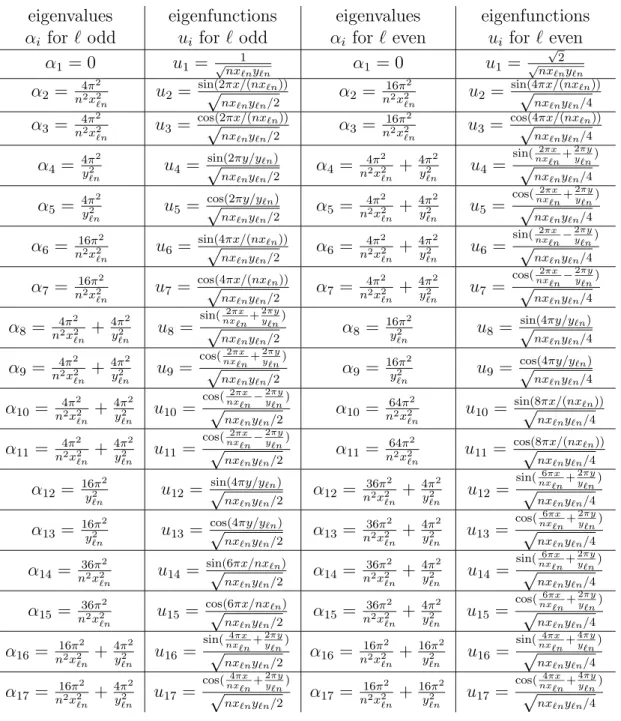
With the aid of Lemma 2 we list 17 of the αi and ui in Table 1.
With the orderings for the eigenvalues as chosen in Table 1, we do not necessarily have
αi ≤ αj for i ≤ j. However, we still have αi ր ∞ as i ր ∞. Choose αρℓ/n(1), αρℓ/n(2),· · ·
the complete set of eigenvalues with multiplicity 1 of the operator −∆ on the flat torusC/Γ
eigenvalues eigenfunctions eigenvalues eigenfunctions
αi for ℓ odd ui for ℓ odd αi for ℓ even ui for ℓ even
α1 = 0 u1 = √nx1ℓnyℓn α1 = 0 u1 = √
2 √nx
ℓnyℓn α2 = 4π
2
n2x2
ℓn u2 =
sin(2√πx/(nxℓn))
nxℓnyℓn/2
α2 = 16π
2
n2x2
ℓn u2 =
sin(4√πx/(nxℓn))
nxℓnyℓn/4 α3 = 4π
2
n2
x2
ℓn u3 =
cos(2√πx/(nxℓn))
nxℓnyℓn/2
α3 = 16π
2
n2
x2
ℓn u3 =
cos(4√πx/(nxℓn))
nxℓnyℓn/4 α4 = 4π
2
y2
ℓn u4 =
sin(2πy/yℓn)
√
nxℓnyℓn/2
α4 = 4π
2
n2x2
ℓn + 4π2
y2
ℓn u4 = sin(2πx
nxℓn+
2πy
yℓn)
√
nxℓnyℓn/4 α5 = 4π
2
y2
ℓn u5 =
cos(2πy/yℓn)
√
nxℓnyℓn/2
α5 = 4π
2
n2
x2
ℓn + 4π2
y2
ℓn u5 =
cos(2πx nxℓn+
2πy
yℓn)
√
nxℓnyℓn/4 α6 = 16π
2
n2x2
ℓn u6 =
sin(4√πx/(nxℓn))
nxℓnyℓn/2
α6 = 4π
2
n2x2
ℓn + 4π2
y2
ℓn u6 = sin(2πx
nxℓn−
2πy
yℓn)
√
nxℓnyℓn/4 α7 = 16π
2
n2x2
ℓn u7 =
cos(4√πx/(nxℓn))
nxℓnyℓn/2
α7 = 4π
2
n2x2
ℓn + 4π2
y2
ℓn u7 =
cos(2πx nxℓn−
2πy
yℓn)
√
nxℓnyℓn/4 α8 = 4π
2
n2
x2
ℓn + 4π2
y2
ℓn u8 = sin(2πx
nxℓn+
2πy
yℓn)
√
nxℓnyℓn/2 α8 = 16π2
y2
ℓn u8 =
sin(4πy/yℓn)
√
nxℓnyℓn/4 α9 = 4π
2
n2x2
ℓn + 4π2
y2
ℓn u9 =
cos( 2πx nxℓn+
2πy
yℓn)
√
nxℓnyℓn/2
α9 = 16π
2
y2
ℓn u9 =
cos(4πy/yℓn)
√
nxℓnyℓn/4 α10 = 4π
2
n2
x2
ℓn + 4π2
y2
ℓn u10=
cos( 2πx nxℓn−
2πy
yℓn)
√
nxℓnyℓn/2
α10 = 64π
2
n2
x2
ℓn u10=
sin(8√πx/(nxℓn))
nxℓnyℓn/4 α11 = 4π
2
n2x2
ℓn + 4π2
y2
ℓn u11=
cos( 2πx
nxℓn−
2πy
yℓn)
√
nxℓnyℓn/2
α11 = 64π
2
n2x2
ℓn u11=
cos(8√πx/(nxℓn))
nxℓnyℓn/4 α12 = 16π
2
y2
ℓn u12=
sin(4πy/yℓn)
√
nxℓnyℓn/2
α12 = 36π
2
n2
x2
ℓn + 4π2
y2
ℓn u12=
sin(6πx nxℓn+
2πy
yℓn)
√
nxℓnyℓn/4 α13 = 16π
2
y2
ℓn u13=
cos(4πy/yℓn)
√
nxℓnyℓn/2
α13 = 36π
2
n2x2
ℓn + 4π2
y2
ℓn u13=
cos(6πx
nxℓn+
2πy
yℓn)
√
nxℓnyℓn/4 α14= 36π
2
n2
x2
ℓn u14=
sin(6√ πx/nxℓn)
nxℓnyℓn/2
α14 = 36π
2
n2
x2
ℓn + 4π2
y2
ℓn u14=
sin(6πx nxℓn+
2πy
yℓn)
√
nxℓnyℓn/4 α15= 36π
2
n2x2
ℓn u15=
cos(6√ πx/nxℓn)
nxℓnyℓn/2
α15 = 36π
2
n2x2
ℓn + 4π2
y2
ℓn u15=
cos(6πx
nxℓn+
2πy
yℓn)
√
nxℓnyℓn/4 α16 = 16π
2
n2
x2
ℓn + 4π2
y2
ℓn u16 = sin(4πx
nxℓn+
2πy
yℓn)
√
nxℓnyℓn/2
α16 = 16π
2
n2
x2
ℓn + 16π2
y2
ℓn u16=
sin(4πx nxℓn+
4πy
yℓn)
√
nxℓnyℓn/4 α17 = 16π
2
n2x2
ℓn + 4π2
y2
ℓn u17=
cos( 4πx nxℓn+
2πy
yℓn)
√
nxℓnyℓn/2
α17 = 16π
2
n2x2
ℓn + 16π2
y2
ℓn u17=
cos(4πx nxℓn+
4πy
yℓn)
√
nxℓnyℓn/4
Table 1:
The first 17 eigenvalues and eigenfunctions of −∆ui =αiui.The first of the following two lemmas follows from the variational characterization for eigenvalues, and the second follows from Lemma 3, the Courant nodal domain theorem, and geometric properties of the surfaces Wℓ/n:
Lemma 4 ([R1], [R2]). Choose µ∈Z+ so that αρ
ℓ/n(µ) <4H. Then Ind(Wℓ/n)≥µ−1.
Lemma 5 ([R1], [R2]). For all n∈Z+, n ≥2we have that Ind(Wℓ/n)≥2n−2 ifℓ is odd,
and Ind(Wℓ/n)≥n−2 if ℓ is even.
4
The lower bound
8
for Ind(
W
ℓ/n)
Numerical Result: Ind(Wℓ/n)≥8 for all ℓ/n.
Observe that, although the eigenvalues ofL depend on the choice ofH, the number of negative eigenvalues is independent of H. So without loss of generality we fixH = 1/2.
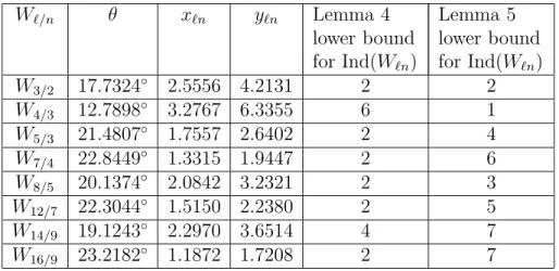
By Lemma 5, Ind(Wℓ/n) can be less than 8 only if ℓ/nis one of 3/2, 4/3, 5/3, 5/4, 7/4,
6/5, 8/5, 8/7, 10/7, 12/7, 10/9, 14/9, or 16/9. Lemma 4 also gives explicit lower bounds for the index, since we know the values of xℓn and yℓn numerically by formula (5), and hence
we know the αρℓ/n(i) (see Table 1). Lemma 4 implies that the index is at least 8 when ℓ/nis
5/4, 6/5, 8/7, 10/7, or 10/9. Thus we only need to consider the following eight surfaces:
W3/2, W4/3, W5/3,W7/4,W8/5, W12/7, W14/9, andW16/9.
For these surfaces we list, in Table 2, the corresponding θ, xℓn, yℓn and lower bounds
for index. These approximate values for θ, xℓn, and yℓn were computed numerically using
formulas (4) and (5) and the software Mathematica. Recall that always θ ∼= 65.354◦.
Wℓ/n θ xℓn yℓn Lemma 4
lower bound for Ind(Wℓn)
Lemma 5 lower bound for Ind(Wℓn)
W3/2 17.7324◦ 2.5556 4.2131 2 2
W4/3 12.7898◦ 3.2767 6.3355 6 1
W5/3 21.4807◦ 1.7557 2.6402 2 4
W7/4 22.8449◦ 1.3315 1.9447 2 6
W8/5 20.1374◦ 2.0842 3.2321 2 3
W12/7 22.3044◦ 1.5150 2.2380 2 5
W14/9 19.1243◦ 2.2970 3.6514 4 7
W16/9 23.2182◦ 1.1872 1.7208 2 7
Table 2:
xℓn, yℓn are computed using the value H= 1/2.We will find specific spaces on which L is negative definite, for these eight surfaces. LetN be an arbitrary positive integer. Consider a finite subset{u˜1 =ui1, . . . ,u˜N =uiN}
of the eigenfunctions ui of −∆ onC/Γ, defined in Section 3, with corresponding eigenvalues
˜
αj =αij, j = 1, . . . , N. If we consider any u= PN
i=1aiu˜i ∈span{u˜1, . . . ,u˜N}, a1, . . . , aN ∈
R, then R
C/ΓuL(u)dx dy = PN
i,j=1ai( ˜αjδij −˜bij)aj, where ˜bij :=
R
C/ΓVu˜iu˜jdxdy. So we
have R
C/ΓuL(u)dx dy < 0 for all nonzero u ∈ span{u˜1, . . . ,u˜N} if and only if the matrix
( ˜αjδij−˜bij)i,j=1,...,N is negative definite. Lemma 3 then implies:
Theorem 1 ([R1], [R2]). If the N×N matrix ( ˜αjδij−˜bij)i,j=1,...,N is negative definite, then
Ind(Wℓ/n)≥N −1.
Table 3:
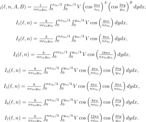
Eigenfunctions of −∆ producing 9-dimensional spaces on which Q is negative definite.Definition 2 Given A, B even integers and ℓ, n ∈ Z+, we now define the following basic
integrals:
I0(ℓ, n, A, B) = nxℓn1yℓn Rxℓn/4
0
Ryℓn/4
0 V
cos2πx xℓn
A
cos2yπy
ℓn B
dydx,
I1(ℓ, n) = nxℓn8yℓn
Rnxℓn/4 0
Ryℓn/4 0 V cos
4πx nxℓn
dydx,
I2(ℓ, n) = nxℓn8yℓn
Rnxℓn/4 0
Ryℓn/4 0 V cos
8πx nxℓn
dydx,
I3(ℓ, n) = nxℓn8yℓn
Rnxℓn/4 0
Ryℓn/4 0 V cos
16πx nxℓnyℓn
dydx,
I4(ℓ, n) = nxℓn8yℓn
Rnxℓn/4 0
Ryℓn/4 0 V cos
4πx nxℓn
cos4yπy
ℓn
dydx,
I5(ℓ, n) = nxℓn8yℓn
Rnxℓn/4 0
Ryℓn/4 0 V cos
4πx nxℓn
cos8πx nxℓn
dydx,
I6(ℓ, n) = nxℓn8yℓn
Rnxℓn/4 0
Ryℓn/4 0 V cos
8πx nxℓn
cos4yπy
ℓn
dydx,
I7(ℓ, n) = nxℓn8yℓn
Rnxℓn/4 0
Ryℓn/4 0 V cos
12πx nxℓn
cos4yπy
ℓn
dydx.
Now, for each surface Wℓ/n given in Table 2, we will fix N = 9 and choose the subset
{u˜1, . . . ,u˜9}such that the matrix ( ˜αjδij−˜bij)i,j=1,...,N is negative definite. These choices are
given in Table 3. With these choices for ˜ui, we have the following lemma:
Lemma 6 With the choices given in Table 3, all elements of the eight matricesM(ℓ, n) := ( ˜αjδij−˜bij)i,j=1,...,9 can be expressed in terms of the basic integrals I0(ℓ, n, A, B)and Ij(ℓ, n)
for A, B even and j = 1,2, . . . ,7.
Proof: The symmetries V(x, y) = V(−x, y) = V(x,−y) = V xℓn 2 −x, y
= V x,yℓn 2 −y
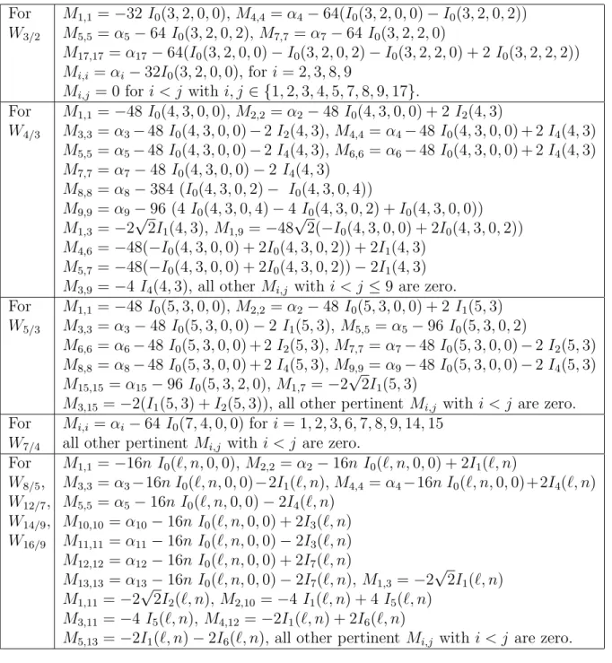
For
W3/2
M1,1 =−32 I0(3,2,0,0),M4,4 =α4−64(I0(3,2,0,0)−I0(3,2,0,2)) M5,5 =α5−64 I0(3,2,0,2),M7,7 =α7 −64 I0(3,2,2,0)
M17,17=α17−64(I0(3,2,0,0)−I0(3,2,0,2)−I0(3,2,2,0) + 2 I0(3,2,2,2)) Mi,i =αi−32I0(3,2,0,0), for i= 2,3,8,9
Mi,j = 0 for i < j with i, j ∈ {1,2,3,4,5,7,8,9,17}.
For
W4/3
M1,1 =−48 I0(4,3,0,0),M2,2 =α2−48 I0(4,3,0,0) + 2I2(4,3)
M3,3 =α3−48I0(4,3,0,0)−2I2(4,3),M4,4 =α4−48I0(4,3,0,0) + 2I4(4,3) M5,5 =α5−48I0(4,3,0,0)−2I4(4,3),M6,6 =α6−48I0(4,3,0,0) + 2I4(4,3) M7,7 =α7−48 I0(4,3,0,0)−2 I4(4,3)
M8,8 =α8−384 (I0(4,3,0,2)− I0(4,3,0,4))
M9,9 =α9−96 (4 I0(4,3,0,4)−4 I0(4,3,0,2) +I0(4,3,0,0)) M1,3 =−2
√
2I1(4,3),M1,9 =−48
√
2(−I0(4,3,0,0) + 2I0(4,3,0,2)) M4,6 =−48(−I0(4,3,0,0) + 2I0(4,3,0,2)) + 2I1(4,3)
M5,7 =−48(−I0(4,3,0,0) + 2I0(4,3,0,2))−2I1(4,3) M3,9 =−4 I4(4,3), all other Mi,j with i < j ≤9 are zero.
For
W5/3
M1,1 =−48 I0(5,3,0,0),M2,2 =α2−48 I0(5,3,0,0) + 2I1(5,3) M3,3 =α3−48 I0(5,3,0,0)−2 I1(5,3),M5,5 =α5−96I0(5,3,0,2)
M6,6 =α6−48I0(5,3,0,0) + 2I2(5,3),M7,7 =α7−48I0(5,3,0,0)−2I2(5,3) M8,8 =α8−48I0(5,3,0,0) + 2I4(5,3),M9,9 =α9−48I0(5,3,0,0)−2I4(5,3) M15,15=α15−96 I0(5,3,2,0),M1,7 =−2
√
2I1(5,3)
M3,15 =−2(I1(5,3) +I2(5,3)), all other pertinent Mi,j with i < j are zero.
For
W7/4
Mi,i =αi−64 I0(7,4,0,0) for i= 1,2,3,6,7,8,9,14,15
all other pertinent Mi,j with i < j are zero.
For
W8/5, W12/7, W14/9, W16/9
M1,1 =−16n I0(ℓ, n,0,0),M2,2 =α2−16n I0(ℓ, n,0,0) + 2I1(ℓ, n)
M3,3 =α3−16n I0(ℓ, n,0,0)−2I1(ℓ, n),M4,4 =α4−16n I0(ℓ, n,0,0)+2I4(ℓ, n) M5,5 =α5−16n I0(ℓ, n,0,0)−2I4(ℓ, n)
M10,10=α10−16n I0(ℓ, n,0,0) + 2I3(ℓ, n) M11,11=α11−16n I0(ℓ, n,0,0)−2I3(ℓ, n) M12,12=α12−16n I0(ℓ, n,0,0) + 2I7(ℓ, n)
M13,13=α13−16n I0(ℓ, n,0,0)−2I7(ℓ, n), M1,3 =−2
√
2I1(ℓ, n) M1,11 =−2
√
2I2(ℓ, n),M2,10=−4I1(ℓ, n) + 4 I5(ℓ, n) M3,11 =−4 I5(ℓ, n),M4,12=−2I1(ℓ, n) + 2I6(ℓ, n)
M5,13 =−2I1(ℓ, n)−2I6(ℓ, n), all other pertinent Mi,j with i < j are zero.
Table 4:
Elements Mi,j of the symmetric matrices M(ℓ, n) expressed in terms of thebasic integrals. We have chosen here to index the Mi,j using the counters associated to αj
and uj, rather than α˜j and u˜j.
By numerical methods, we can estimate that all of the relevant Ij(ℓ, n) for j ≥ 1 are
approximately zero, and that
I0(3,2,0,0)∼= 0.2968, I0(3,2,2,0)∼= 0.2304, I0(3,2,0,2)∼= 0.2408, I0(3,2,2,2)∼= 0.1947,
I0(4,3,0,0)∼= 0.1077, I0(4,3,0,2)∼= 0.0776, I0(4,3,0,4)∼= 0.0667, I0(5,3,0,0)∼= 0.4532,
I0(5,3,2,0)∼= 0.3910, I0(5,3,0,2)∼= 0.4046, I0(7,4,0,0)∼= 0.6072, I0(8,5,0,0)∼= 0.1878,
These values were computed with a Mathematica program using the NIntegrate and Jaco-biCN commands, and the program is available at the web site of the third author. One note of warning is that Mathematica has different conventions than Walter’s paper, and hence
cnk in [Wa] is equivalent to cnk2 in Mathematica. We include a sample of our code in the
Appendix.
Now we can make approximations for the eight matricesM(ℓ, n). The matrix M(3,2) is approximately
M(3,2)≈
−9.50 0 0 0 0 0 0 0 0
0 −7.99 0 0 0 0 0 0 0
0 0 −7.99 0 0 0 0 0 0
0 0 0 −1.36 0 0 0 0 0
0 0 0 0 −13.2 0 0 0 0
0 0 0 0 0 −8.70 0 0 0
0 0 0 0 0 0 −5.76 0 0
0 0 0 0 0 0 0 −5.76 0
0 0 0 0 0 0 0 0 −5.50
,
and all nondiagonal terms are known to be zero by rigorous mathematical computation, and all nonzero entries have been computed only numerically.
M(4,3) is approximately the nondiagonal matrix
M(4,3)≈
−5.17 0 O 0 0 0 0 0 −3.23
0 −3.53 0 0 0 0 0 0 0
O 0 −3.53 0 0 0 0 0 O
0 0 0 −3.78 0 −2.29 0 0 0
0 0 0 0 −3.78 0 −2.29 0 0
0 0 0 −2.29 0 −3.78 0 0 0
0 0 0 0 −2.29 0 −3.78 0 0
0 0 0 0 0 0 0 −0.25 0
−3.23 0 O 0 0 0 0 0 −2.21
,
and again here all entries that are 0 have been computed mathematically rigorously, and all nonzero entries have been computed only numerically. The symbol O denotes an entry that has been computed numerically to be approximately zero, but not mathematically rigorously. We shall continue to use these conventions in all remaining matrices.
M(5,3) is approximately the diagonal matrix
M(5,3)≈
−21.8 0 0 0 0 O 0 0 0
0 −20.3 0 0 0 0 0 0 0
0 0 −20.3 0 0 0 0 0 O
0 0 0 −33.2 0 0 0 0 0
0 0 0 0 −16.1 0 0 0 0
O 0 0 0 0 −16.1 0 0 0
0 0 0 0 0 0 −14.7 0 0
0 0 0 0 0 0 0 −14.7 0
0 0 O 0 0 0 0 0 −24.7
M(7,4) is approximately the diagonal matrix
M(7,4)≈
−38.9 0 0 0 0 0 0 0 0
0 −37.5 0 0 0 0 0 0 0
0 0 −37.5 0 0 0 0 0 0
0 0 0 −33.3 0 0 0 0 0
0 0 0 0 −33.3 0 0 0 0
0 0 0 0 0 −27.0 0 0 0
0 0 0 0 0 0 −27.0 0 0
0 0 0 0 0 0 0 −26.3 0
0 0 0 0 0 0 0 0 −26.3
.
M(8,5) is approximately the diagonal matrix
M(8,5)≈
−15.0 0 O 0 0 0 O 0 0
0 −13.6 0 0 0 O 0 0 0
O 0 −13.6 0 0 0 O 0 0
0 0 0 −10.9 0 0 0 O 0
0 0 0 0 −10.9 0 0 0 O
0 O 0 0 0 −9.2 0 0 0
O 0 O 0 0 0 −9.2 0 0
0 0 0 O 0 0 0 −8.0 0
0 0 0 0 O 0 0 0 −8.0
.
M(12,7) is approximately the diagonal matrix
M(12,7)≈
−29.7 0 O 0 0 0 O 0 0
0 −28.3 0 0 0 O 0 0 0
O 0 −28.3 0 0 0 O 0 0
0 0 0 −21.5 0 0 0 O 0
0 0 0 0 −21.5 0 0 0 O
0 O 0 0 0 −24.1 0 0 0
O 0 O 0 0 0 −24.1 0 0
0 0 0 O 0 0 0 −18.7 0
0 0 0 0 O 0 0 0 −18.7
.
M(14,9) is approximately the diagonal matrix
M(14,9)≈
−12.1 0 O 0 0 0 O 0 0
0 −11.7 0 0 0 O 0 0 0
O 0 −11.7 0 0 0 O 0 0
0 0 0 −9.1 0 0 0 O 0
0 0 0 0 −9.1 0 0 0 O
0 O 0 0 0 −10.6 0 0 0
O 0 O 0 0 0 −10.6 0 0
0 0 0 O 0 0 0 −8.3 0
0 0 0 0 O 0 0 0 −8.3
M(16,9) is approximately the diagonal matrix
M(16,9)≈
−49.2 0 O 0 0 0 O 0 0
0 −47.9 0 0 0 O 0 0 0
O 0 −47.9 0 0 0 O 0 0
0 0 0 −35.6 0 0 0 O 0
0 0 0 0 −35.6 0 0 0 O
0 O 0 0 0 −43.7 0 0 0
O 0 O 0 0 0 −43.7 0 0
0 0 0 O 0 0 0 −32.8 0
0 0 0 0 O 0 0 0 −32.8
.
All eight of these matrices are 9×9 and negative definite. Hence Theorem 1 implies the numerical result.
5
Appendix: the Mathematica code
The following is a Mathematica code for computing the values I0(4,3,0,0), I0(4,3,0,2), I0(4,3,0,4), I1(4,3), I2(4,3), I4(4,3), and the elements of the matrix M(4,3). The seven
other needed codes for different ℓ and n were written similarly.
H = 1/2; k1 = Sin[theta1]; k2 = Sin[theta2];
gamma1 = Sqrt[Tan[theta1]]; gamma2 = Sqrt[Tan[theta2]]; alpha1 = Sqrt[4 H Sin[2theta2]/Sin[2(theta1 + theta2)]]; alpha2 = Sqrt[4 H Sin[2theta1]/Sin[2(theta1 + theta2)]];
F = 4ArcTanh[gamma1 gamma2 JacobiCN[alpha1 x, k1^2] JacobiCN[alpha2 y, k2^2]]; V = 4 H Cosh[F];
ell = 4; n = 3;
theta1 = 2 Pi (12.7898/360); theta2 = 2 Pi (65.354955354/360); x0 = 3.2767; y0 = 6.3355;
Print["I_0(4,3,0,0) is ",I0x4c3c0c0x = (1/(n x0 y0)) NIntegrate[ V , {x, 0, x0/4}, {y, 0, y0/4}]];
Print["I_0(4,3,0,2) is ",I0x4c3c0c2x = (1/(n x0 y0)) NIntegrate[
V (Cos[2 Pi x/x0])^0(Cos[2 Pi y/y0])^2,{x, 0, x0/4}, {y, 0, y0/4}]];
Print["I_0(4,3,0,4) is ",I0x4c3c0c4x = (1/(n x0 y0)) NIntegrate[
V (Cos[2 Pi x/x0])^0(Cos[2 Pi y/y0])^4,{x, 0, x0/4}, {y, 0, y0/4}]];
Print["I_1(4,3) is ",I1x4c3x = (8/(n x0 y0)) (NIntegrate[
V (Cos[4 Pi x/(n x0)]),{x, 0, x0/4}, {y, 0, y0/4}] + NIntegrate[ V (Cos[4 Pi x/(n x0)]),{x, x0/4, 2 x0/4}, {y, 0, y0/4}] + NIntegrate[ V (Cos[4 Pi x/(n x0)]),{x, 2 x0/4, n x0/4}, {y, 0, y0/4}])];
Print["I_2(4,3) is ",I2x4c3x = (8/(n x0 y0)) (NIntegrate[
Print["I_4(4,3) is ",I4x4c3x = (8/(n x0 y0)) (NIntegrate[
V (Cos[4 Pi x/(n x0)]) (Cos[4 Pi y/y0]),{x,0,x0/4},{y,0,y0/4}]+NIntegrate[ V (Cos[4 Pi x/(n x0)]) (Cos[4 Pi y/y0]),{x,x0/4,2 x0/4},{y,0,y0/4}]+NIntegrate[ V (Cos[4 Pi x/(n x0)]) (Cos[4 Pi y/y0]),{x, 2 x0/4, n x0/4}, {y, 0, y0/4}])];
aa = 0; bb = 0; alpha1 = aa(4 N[Pi^2]/(n^2 x0^2)) + bb (4 N[Pi^2]/(y0^2));
aa = 4; bb = 0; alpha2 = aa(4 N[Pi^2]/(n^2 x0^2)) + bb (4 N[Pi^2]/(y0^2)); alpha3 = alpha2;
aa = 1; bb = 1; alpha4 = aa(4 N[Pi^2]/(n^2 x0^2)) + bb (4 N[Pi^2]/(y0^2)); alpha5 = alpha4; alpha6 = alpha4; alpha7 = alpha4;
aa = 0; bb = 4; alpha8 = aa(4 N[Pi^2]/(n^2 x0^2)) + bb (4 N[Pi^2]/(y0^2)); alpha9 = alpha8;
Print["M(1,1) is ", -48 I0x4c3c0c0x];
Print["M(2,2) is ", alpha2 - 48 I0x4c3c0c0x]; Print["M(3,3) is ", alpha3 - 48 I0x4c3c0c0x]; Print["M(4,4) is ", alpha4 - 48 I0x4c3c0c0x]; Print["M(5,5) is ", alpha5 - 48 I0x4c3c0c0x]; Print["M(6,6) is ", alpha6 - 48 I0x4c3c0c0x]; Print["M(7,7) is ", alpha7 - 48 I0x4c3c0c0x];
Print["M(8,8) is ", alpha8 - 384 (I0x4c3c0c2x - I0x4c3c0c4x)];
Print["M(9,9) is ", alpha9 - 96 (I0x4c3c0c0x + 4 I0x4c3c0c4x - 4 I0x4c3c0c2x)]; Print["M(1,9) is ", -48 N[Sqrt[2]] (-I0x4c3c0c0x + 2 I0x4c3c0c2x)];
Print["M(4,6) is ", -48 (-I0x4c3c0c0x + 2 I0x4c3c0c2x)]; Print["M(5,7) is ", -48 (-I0x4c3c0c0x + 2 I0x4c3c0c2x)];
References
[A] U. ABRESCH,Constant mean curvature tori in terms of elliptic functions, J. reine u. angew Math.374 (1987), 169-192.
[BC] L. BARBOSA, M. do CARMO, Stability of hypersurfaces with constant mean curvature, Math. Z.185 (1984), 339–353.
[CP] M. do CARMO, C. K. PENG, Stable minimal surfaces in R3 are planes, Bull. Amer. Math.
Soc.1(1979), 903–906.
[FC] D. FISCHER-COLBRIE, On complete minimal surfaces with finite Morse index in three manifolds, Invent. Math. 82(1985), 121–132.
[H] H. HOPF, Differential geometry in the large, Lecture Notes in Math. 1000 Springer-Verlag (1983).
[LR] F. J. LOPEZ, A. ROS, Completenimal surfaces with index one and stable constant mean curvature surfaces, Comment. Math. Helvetici 64(1989), 34–43.
[R2] W. ROSSMAN, Wente Tori and Morse Index, An. Acad. Bras. Ci.71(4)(1999), 607–613.
[Si] A. M. SILVEIRA, Stability of complete noncompact surfaces with constant mean curvature, Math. Ann.277(1987), 629–638.
[Sp] J. SPRUCK,The elliptic sinh-Gordon equation and the construction of toroidal soap bubbles, Lecture Notes in Math.1340 Springer-Verlag (1988), 275–301.
[Wa] R. WALTER, Explicit examples to the H-problem of Heinz Hopf, Geometriae Dedicata 23
(1987), 187–213.
[We] H. WENTE, Counterexample of a conjecture of H. Hopf, Pacific J. Math. 121 (1986), 193– 243.
Levi Lopes de Lima, Departamento de Matem´atica, Universidade Federal do Cear´a Campus do Pici, 60455–760 Fortaleza, Brazil, levi@mat.ufc.br
Vicente Francisco de Sousa Neto, Departamento de Matem´atica
Universidade Cat´olica de Pernambuco, Recife, Brazil, vicente@unicap.br
Wayne Rossman, Department of Mathematics, Faculty of Science