A CCO-based Sigma-Delta ADC

(1)

Bruno Miguel Rosa Ferreira

Licenciado em Ciências da

Engenharia Eletrotécnica e de Computadores

A CCO-based Sigma-Delta ADC

Dissertação para Obtenção do Grau de Mestre em Engenharia Eletrotécnica e de Computadores

Orientador: Prof. Dr. Luís Augusto Bica Gomes de Oliveira, Professor Auxiliar com Agregação, Universidade Nova de Lisboa Setembro de 2018

(2)

(3)

A CCO-based Sigma-Delta ADC

A Faculdade de Ciências e Tecnologia e a Universidade Nova de Lisboa têm o direito, perpétuo e sem limites geográficos, de arquivar e publicar esta dissertação através de exemplares impressos reproduzidos em papel ou de forma digital, ou por qualquer outro meio conhecido ou que venha a ser inventado, e de a divulgar através de repositórios científicos e de admitir a sua cópia e distribuição com objetivos educacionais ou de investigação, não comerciais, desde que seja dado crédito ao autor e editor.

(4)

(5)

(6)

(7)

Acknowledgments

In this section I would like to thank everyone that helped me and supported me through this last five years of college.

First, I would like to thank to my supervisor, professor Luís Oliveira for the possibility of developing this dissertation and for the availability (at practically anytime), for the commitment and the enthusiastic way of helping when problems came up. I would like to thank you the opportunity of helping in Electrónica II classes too, which was a very enriching experience for me.

I thank to professor Maria Helena Fino for the multiple advices and for the opportunity of helping in Teoria de Circuitos Elétricos classes, which was my first experience as class monitor.

I have to thank professor João Goes for the advises that were very useful for the development of this dissertation.

I would, also, like to thank the faculty of the Departamento de Engenharia Eletrotécnica for teaching me so much these last five years.

Miguel Fernandes, I thank you for the help you gave me while developing the work for this dissertation and I wish you luck to conclude your PhD.

To my friends and colleagues, Didier Lopes, Nuno Baptista, Pedro Rodrigues and João Pires, I thank you for being so easy to work with you and I wish you all the best.

I thank to my bandmates Alexandre Casimiro, Jorge Lourenço, Ricardo Matias, Tiago David, Rafael Santos and Duarte Fernandes for the support and friendship and for always being prepared to play some Rock n’ Roll, that helped me on clearing my mind when needed.

(8)

Acknowledgments

I would like to thank to a very special friend named Mimi, for making me company every night of writing. Even though “she” is not human, sometimes seems very close to that.

I cannot thank enough to my girlfriend, Mafalda Amarelo for all the emotional support, advise, company, love,… I might even write a dissertation with all that you do for me. Thank you so much.

My brother, Jorge Ferreira, I thank you for having the greatest faith in me and for being so supportive of my decisions.

To my parents, Maria Rosa and Osvaldo Ferreira, I thank you for supporting me in everything. Without you, I would never done it. Aos meus pais, Maria Rosa e Osvaldo Ferreira, eu agradeço por me apoiarem em tudo. Sem vocês não teria conseguido.

(9)

Abstract

Analog-to-digital converter (ADC) is one of the most important blocks in nowadays systems. Most of the data processing is done in the digital domain however, the physical world is analog. ADCs make the bridge between analog and digital domain.

The constant and unstoppable evolution of the technology makes the dimensions of the transistors smaller and smaller, and the classical solutions of Sigma-Delta converters (ΣΔ) are becoming more challenging to design because they normally require high active gain blocks difficult to achieve in modern technologies.

In recent years, the use of voltage-controlled oscillators (VCO) in ΣΔ converters has been widely explored, since they are used as quantizers and their implementations are mostly made with digital blocks, which is preferable with new technologies.

In this work a second-order ΣΔ modulator based on two current-controlled oscillators (CCO) with a single output phase and an independent phase generator for each CCO that generates any desired number of phases using the oscillation of its CCO as reference has been proposed.

This ΣΔ modulator was studied through a MATLAB/Simulink®_{model, obtaining}

promising results with the SNDR in the order of 75 dB, at a sampling frequency of 1 GHz, and a bandwidth of 5 MHz, corresponding to an ENOB of, approximately, 12 bits.

Keywords: Sigma-Delta, ADC, DAC, CCO-based ADC, VCO-based ADC, analog-to-digital converter, digital-to-analog

(10)

(11)

Resumo

O conversor analógico-digital (ADC) é um dos blocos mais importantes dos sistemas da atualidade. A maioria do processamento de dados é feito no domínio digital, no entanto, o mundo físico é analógico. Os ADCs fazem a ponte entre o domínio analógico e digital.

A constante e imparável evolução da tecnologia faz com que as dimensões dos transístores sejam cada vez mais pequenas e que as soluções clássicas de conversores Sigma-Delta (ΣΔ) sejam cada vez mais difíceis de projetar por necessitarem, normalmente, de blocos com ganhos ativos elevados, que são cada vez mais difíceis de projetar com tecnologias recentes.

Nos últimos anos o uso de osciladores controlados por tensão (VCO) em conversores ΣΔ tem sido amplamente explorado, uma vez que estes usados como quantizadores e as suas implementações são maioritariamente feitas com blocos digitais. O que é preferível com as novas tecnologias.

Neste trabalho propõe-se um modulador ΣΔ de segunda ordem baseado dois osciladores controlados por corrente (CCO) com uma só fase de saída e um gerador de fases independente por cada CCO, que gera um qualquer número de fases desejado usando a oscilação do seu CCO como referência.

Este modulador ΣΔ foi estudado através de um modelo de MATLAB/Simulink®_,

obtendo-se resultados promissores com a SNDR na ordem dos 75 dB, para uma frequência de amostragem de 1 GHz, e uma largura de banda de 5 MHz, o que corresponde a um ENOB de, aproximadamente, 12 bits.

Palavras-chave: Sigma-Delta, ADC, DAC, baseado em CCO ADC, baseado em VCO, ADC, conversor analógico-digital, digital-analógico

(12)

(13)

List of Tables

Table 2.1: Comparison of state of the art VCO-based CT ΔΣ modulator ADCs ... 21

Table 3.1: CCO transistor sizing ... 26

Table 3.2: Phase Noise of the implemented CCO ... 27

Table 3.3: CCO results ... 27

Table 4.1: Description of simulation tests ... 36

Table 4.2: 7-phase ADC parameters and SNR results... 40

Table 4.5: First simulation results (ref. KCCO=7.2 GHz/A linear, 20dB filter, 0% mismatch) ... 48

Table 4.6: Second simulation results (ref. KCCO=7.2 GHz/A linear, 20dB filter, 1% mismatch) ... 49

Table 4.7: Third simulation results (ref. KCCO=7.2 GHz/A linear, 0dB filter, 0% mismatch) ... 49

Table 4.8: Forth simulation results (ref. KCCO=1 GHz/A linear, 20dB filter, 0% mismatch) ... 50

Table 4.9: Fifth simulation results (ref. KCCO=7.2 GHz/A non-linear, 20dB filter, 0% mismatch) ... 50

Table 4.10: Last simulation results (ref. KCCO=7.2 GHz/A non-linear, 20dB filter, 1% mismatch) ... 51

(16)

(17)

List of Figures

Figure 2.1: Sinusoidal oscillator output ... 4

Figure 2.2: Positive feedback block diagram ... 4

Figure 2.3: Output spectrum of an oscillator with phase noise ... 5

Figure 2.4: Q definition for second order system ... 6

Figure 2.5: Typical asymptotic noise spectrum of an oscillator output... 7

Figure 2.6: Basic LC-VCO ... 8

Figure 2.7: Relaxation Oscillator... 9

Figure 2.8: Typical ring-oscillator ... 9

Figure 2.9: ΔΣM ... 10

Figure 2.10: PSD of ADC quantization noise ... 11

Figure 2.11: Noise transfer function of different orders of noise shaping in ΔΣM ... 13

Figure 2.12: SNR, SNDR and DR of a ΔΣM ... 14

Figure 2.13: VCO-based quantizer ... 16

Figure 2.14: VCO-based quantizer using the VCO frequency as output ... 16

Figure 2.15: ΣΔ feedback to suppress VCO linearity and quantization errors ... 17

Figure 2.16: VCO-based CT Σ∆ ADC using the VCO phase as quantized output ... 18

Figure 2.17: Differential CCO-based CT ΔΣ ADC ... 19

Figure 2.18: CCO-based CT ΔΣM with passive integrator and capacitive feedback .... 19

Figure 2.19: VCO-based ΔΣM with residue cancelling ... 20

Figure 2.20: VCO-based ADC with combined frequency and phase feedback ... 20

Figure 3.1: Schmitt-trigger ... 24

Figure 3.2: Relaxation Oscillator... 24

Figure 3.3: Cascode current mirror ... 25

Figure 3.4: CCO ... 26

Figure 3.5: Phase Noise of the implemented CCO ... 27

Figure 3.6: Phase Generator ... 28

(18)

List of Figures

Figure 4.1: Proposed Architecture ... 32

Figure 4.2: Output spectrum in ideal conditions (only quantization noise) ... 32

Figure 4.3: Thermometer DAC with 1% mismatch: (a) Output spectrum; (b) DAC cell selection pattern ... 33

Figure 4.4: Natural rotative DAC with 1% mismatch: (a) Output spectrum; (b) DAC cell selection pattern ... 34

Figure 4.5: Natural rotative DAC with 25% mismatch: Output spectrum ... 35

Figure 4.6: Output spectrum of ADC with 7-phase generator (ideal test) ... 37

Figure 4.7: Output spectrum of ADC with 7-phase generator (0 dB of filter gain) ... 37

Figure 4.8: Output code of ADC with 7-phase generator (1% DAC mismatch, non-linear KCCO) ... 38

Figure 4.9: Output spectrum of ADC with 7-phase generator (1% DAC mismatch, non-linear KCCO) ... 39

Figure 4.10: Dynamic range of ADC with 7-phase generator (1% DAC mismatch, non-linear KCCO) ... 39

Figure 4.14: Output spectrum of ADC with 15-phase generator (1% DAC mismatch, non-linear KCCO) ... 43

Figure 4.19: Output spectrum of ADC with 25-phase generator (1% DAC mismatch and non-linear KCCO) ... 47

(19)

Acronyms

ADC Analog-to-Digital Converter

BW Bandwidth

CMOS Complementary Metal–Oxide–Semiconductor CCO Current-Controlled Oscillator

CLA Clocked Averaging

CT Continuous-Time

DAC Digital-to-Analog Converter DEM Dynamic Element Matching

DR Dynamic Range

DWA Data Weighted Average ENOB Effective Number of Bits

IEEE Institute of Electrical and Electronics Engineers OSR Oversampling Ratio

PSD Power Spectral Density Σ∆M Sigma-Delta Modulator

SNDR Signal-to-Noise-and-Distortion Ratio SNR Signal-to-Noise Ratio

(20)

Acronyms

SQNR Signal-to-Quantization-Noise Ratio STF Signal Transfer Function

THD Total Harmonic Distortion VCO Voltage-Controlled Oscillator

(21)

1 Introduction

In this chapter, a brief introduction to subjects related to the work accomplished is done. First, the identification of the problem that this work intends to address as well as the motivation to address it. Second, the contributions of the solution found. And last, the organization of this dissertation.

1.1 Motivation

XXI century’s society has a never-ending hunger for technology. And today’s technology is performing computational and signal processing tasks mostly in the digital domain [1]. This is due to how robust digital circuits are, and how simple and small the implementations are. This small and simple circuits can perform simple tasks on their own, but when multiple cells are combined, more complex tasks can be performed. The main problem of the digital domain is dealing with the physical world, that, unfortunately for digital circuits, is analog. And that is why the analog-to-digital converters (ADCs) are so important in today’s systems. To make the bridge between real world and current day technology.

The ΣΔ ADC is one of the most common architectures, since it can achieve high resolutions with low complexity. However, a classical ΣΔ ADC depends on high gain loop filters to shape the quantization noise to higher frequencies, away from the signal bandwidth. Furthermore, the transistors have less intrinsic gain as CMOS technologies advance, what makes the design of classical ΣΔs more challenging. But with smaller transistors, the switching capacity increases as the timing resolution. For that reason,

(22)

1 Introduction

VCO-based ΣΔ ADCs are becoming more and more popular, since they rely on timing resolution [2]. Also, this architecture can be implemented with mostly digital blocks, decreasing the need for high gain analog blocks.

1.2 Contributions

The main contribution of this dissertation was the study and modulation of an innovating architecture. In which a single-phase current-controlled oscillator (CCO) was used with a separated phase generator that produced the required number of phases desired for the quantization process from one reference CCO. This implements a multi-phase CCO. Two instances of this multi-phase generator are needed in this work.

In this study several sets of conditions were simulated for three resolutions (3, 4 and 4.7-bit), in order to understand the limits of the proposed architecture.

A CCO based on a relaxation oscillator were, also, designed and implemented. While carrying out this dissertation a paper named “Impact of VCO Non-Linearities on VCO-based” were also published on 2nd International Young Engineers Forum on Electrical and Computer Engineering.

1.3 Dissertation Structure

This dissertation is organized as follows:

• Chapter 2 is a literature review of fundamental concepts for the development of the proposed work. With a study on oscillators and ΣΔ ADCs, traditional and VCO-based;

• Chapter 3 describes the CCO designed and the multi-phase generator at first, and finishes with the results obtained for these two components;

• Chapter 4 explains the proposed architecture of a CCO-based ΣΔ ADC first. It also contains all the results for the simulations carried out for the proposed architecture and discussion of these.

• At last, Chapter 5 contains some conclusions that were possible to extract from the work accomplished as well as some future work proposals.

(23)

2 State of the art of VCO-based ΔΣM ADC

In this chapter is presented a literature review on fundamental concepts for the development of the work. First, a study on oscillators concepts and topologies. Second, a study of the fundamentals of ΣΔ modulation. Finally, a VCO-based ΣΔ ADCs study was made, with some examples of recent approaches to the concept as well as comparison of these recent works.

2.1 Oscillators

In VCO or CCO-based ADCs the oscillator is crucial part responsible for the quantization. An oscillator is a circuit capable of producing periodic signals with a fixed frequency. This AC signals are produced depending in a DC input.

The oscillators can be considered linear or non-linear depending on the type of wave produced. The linear oscillators can produce sinusoidal signals and respect the Barkhausen criterion. The non-linear oscillators do not respect the Barkhausen criterion [3] and are typically RC active circuits that can generate different waveforms. These are the type of oscillators desirable for integrated circuitry, since they do not use inductors that occupies large areas. However, active RC oscillators produce more phase noise.

2.1.1 Barkhausen Criterion

Sinusoidal output oscillators produce a sinusoid wave with frequency ω0 and amplitude

V0, which output can be described by:

(24)

2 State of the art of VCO-based ΔΣM ADC

where θ represents the initial phase of the sinusoid.

Figure 2.1 shows the sinusoidal output in time and frequency domain. The sinusoidal oscillators can also be analyzed as positive feedback system like the one in Figure 2.2.

(a) (b)

Figure 2.1: Sinusoidal oscillator output: (a) Time domain; (b) Frequency domain [3]

Figure 2.2: Positive feedback block diagram

The transfer function of the feedback system is given by: 𝑌(𝑗𝜔)

𝑋(𝑗𝜔)=

𝐴(𝑗𝜔)

1 − 𝐴(𝑗𝜔)β(jω) (2.2)

The Barkhausen criterion consists in two conditions about the loop gain that ensures a steady-state oscillation with a frequency ω0. The loop gain must be unity (gain

condition), and the open-loop phase shift must be 2nπ, where n is an integer including zero (phase condition) [3]. The following equations describe the criterion:

|𝐴(𝑗𝜔0)𝛽(𝑗𝜔0)| = 1 (2.3)

(25)

2.1 Oscillators

The conditions of Barkhausen ensures a stable oscillation. However, when booting the oscillator, the loop gain as to be bigger than one to make an instable system that is triggered by noise.

2.1.2 Phase Noise

The noise generated at the output of the oscillator causes variations of the output amplitude and phase. Theses variations are responsible for the appearing of bands around ω0 and its harmonics as shown in Figure 2.3.

Figure 2.3: Output spectrum of an oscillator with phase noise [3]

The oscillator noise can be described in frequency domain, the phase noise, and in time domain, correspondent to the jitter. A common way to quantify the noise is in terms of the single sideband noise spectral density, L(ωn), expressed in decibels below the

carrier per hertz (dBc/Hz) and is given by:

𝐿(𝜔_𝑚) =𝑃(𝜔𝑚)

𝑃(𝜔_𝑜) (2.5)

where P(ω0) is the carrier power, and the P(ωn) is the single sideband noise power at a

distance of ωm from thecarrier in a 1 Hz bandwidth.

2.1.3 Quality Factor (Leeson- Cutler)

The quality factor (Q) is the most used figure of merit for oscillators [3], and it is directly related total phase noise of the oscillator. There are three definitions of it. One of them is the Leeson definition that considers a single resonator network with -3 dB bandwidth B and resonance frequency ω0, shown in Figure 2.4, and given by:

𝑄 =𝜔0

(26)

Figure 2.4: Q definition for second order system [3]

2.1.4 Leeson-Cutler Phase-Noise Equation

The most used phase-noise model is the Leeson-Cutler semi empirical equation [3], that is given by: 𝐿(𝜔_𝑚) = 10 log {2𝐹𝑘𝑇 𝑃_𝑆 [1 + ( 𝜔0 2𝑄𝜔_𝑚) 2 ] (1 +𝜔1/𝑓3 |𝜔𝑚| )} (2.7) where: k – Boltzman constant; T – absolute temperature;

PS – average power dissipated in the resistive part of the tank;

𝜔₀ – oscillation frequency; Q – quality factor;

ωm – offset from the carrier;

𝜔_1/𝑓3 – corner frequency between 1/f3 and 1/f2 zones of the noise spectrum F – empirical parameter, called excess noise factor

Figure 2.5 shows a typical asymptotic noise spectrum of an oscillator output, with three different regions:

(27)

2.1 Oscillators

• (2) The region between ω1 and ω2, that is affected by the modulation frequency of the oscillator by its white noise sources, with a -20 dB/decade slope.

• (3) The area near the carrier frequency, has a -30 dB/decade slope due to 1/f noise of the active devices.

Figure 2.5: Typical asymptotic noise spectrum of an oscillator output [3]

2.1.5 VCO and CCO

A voltage-controlled oscillator (VCO) is a circuit that generates an oscillatory signal with a frequency controlled by an input voltage (𝑉𝑐𝑡𝑟𝑙).

There are two main types of voltage-controlled oscillators for integrated design, the LC oscillators and ring oscillators.

The VCO output is generally given by:

𝑉𝐶𝑂𝑜𝑢𝑡(𝑡) = 𝑉0sin(𝜔𝑐𝑡 + 𝜑) (2.8)

where 𝜑 is the phase, 𝑉₀ is the amplitude of the output wave, and 𝜔_𝑐 angular carrier frequency:

𝜔_𝑐(𝑉𝑐𝑡𝑟𝑙) = 2𝜋𝑓𝑐(𝑉𝑐𝑡𝑟𝑙) (2.9)

dependent in the tuning voltage (𝑉_{𝑐𝑡𝑟𝑙}).

The current-controlled oscillator (CCO) is similar to the VCO, but the oscillation frequency is controlled by an input current. The main advantage of CCOs over VCOs is the much superior linearity on the output frequency. This is due to current being directly related to how fast charge moves. This movement sets the output frequency [4].

(28)

2.1.6 Oscillator examples

LC Oscillators

Figure 2.6 shows an example of this approach and it is basically a capacitor C in parallel with an inductor L to build a resonance tank and resistor with negative value (-R) to compensate the losses of the inductor. The capacitance C is proportional to the tuning voltage (𝑉𝑐𝑡𝑟𝑙), making it behave like a VCO.

The LC oscillators are commonly used in high frequency applications. The inductors involved occupy large areas compared to the ring oscillator, what is not a good practice in integrated circuit design [5].

Figure 2.6: Basic LC-VCO (adapted from [5])

LC oscillators have a limited tuning range but have less phase noise than ring oscillators and lower power consumption.

Also, being a linear oscillator the Barkhausen criterion can be applied for sizing of the oscillator.

Relaxation Oscillators

The relaxation oscillator is basically an integrator and a Schmitt-trigger as shown in Figure 2.7(a). The Schmitt-trigger controls the direction of the integration, maintaining the direction of the integration until a certain value and inverting it until it reaches another value, repeating the process. Figure 2.7(b) shows the waveforms of this kind of oscillator. The output of the Schmitt-trigger is a square wave with two possible values, leading the integrator output to be a triangular wave.

This class of oscillators are not linear, meaning that the Barkhausen criterion cannot be applied.

(29)

2.1 Oscillators

(a) (b)

Figure 2.7: Relaxation Oscillator: (a) block diagram; (b) oscillator waveforms [3]

Ring Oscillators

In Figure 2.8 is represented a typical ring oscillator, which consists in a series of inverters cascade connected. The oscillation is obtained if a phase shift of 180° in total is achieved to form a positive feedback. Each inverter, also called delay cell, has an intrinsic delay associated and the sum of all them is what make the circuit oscillate at a certain frequency. In this single-ended example an odd number of inverters must be used to achieve oscillation. In a fully differential structure an even number of inverters can be used as long as the connection between two are inverted. The tuning is normally done by the voltage supply of the inverters.

Figure 2.8: Typical ring-oscillator: (a) single ended; (b) fully differential (adapted from [6])

The ring oscillator has a wide tuning range and occupies a very small area; however, phase noise and power consumption are typically higher than the LC oscillators.

Ring oscillators are preferable for VCO-based due to the multiple phases that are available in this kind of oscillators as explained in Section 2.3.

(a)

(30)

2.2 Basis of sigma-delta modulation (ΣΔM)

Sigma-delta modulators (Figure 2.9) are the most commonly used oversampling data converters. This kind of converters use a sampling frequency, 𝑓𝑆, much higher than the

Nyquist rate (twice de bandwidth of the modulator, 𝑓_𝐵), by a factor of 8 to 512 times, usually [1]. This factor is called oversampling ratio (OSR) and is given by:

𝑂𝑆𝑅 = 𝑓𝑆 2 × 𝑓𝐵

(2.10) Over Nyquist rate converters, ΔΣ modulators are superior in the following aspects: • Relieve the requirements of analog circuitry, but are reliant on complex digital circuits, which is desirable for modern CMOS technologies, with less intrinsic gain and lower power supplies.

• The high sample rate of the data converter shifts the image components far away from the bandwidth of the desired signal, thus, reducing the requirements of anti-aliasing filters.

• The quantization noise power can be reduced by increasing the over sampling ratio (OSR) what increase the resolution of the ADC.

(a)

(31)

2.2 Basis of sigma-delta modulation (ΣΔM)

The modulator is a feedback loop containing an ADC and a DAC, both with low resolution, and a loop filter in the forward path, typically, an integrator, as shown in Figure 2.9 a). Even though, the modulator is not linear, it can be approximated by linear model [1] to ease the analysis, as shown in Figure 2.9 b).

2.2.1 Quantization error

Assuming only the effects of quantization error generated by the ADC. If the input signal is constantly changing, it is possible to approximate the quantization error 𝑒𝑄(𝑡) to a

random variable varying between ±Δ/2, with Δ being the difference between two consecutive levels of quantization, otherwise known as step of the ADC. This is equivalent to a white noise source [7] and the power spectral density (PSD) of the total quantization noise power 𝑆_𝑄(𝑓) is an uniform distribution as well, as observable in Figure 2.10 and given by:

𝑆_𝑄(𝑓) = 1 𝐹_𝑠[ 1 Δ∫ 𝑒𝑄 2_𝑑𝑒 𝑄 Δ/2 −Δ/2 ] = Δ 2 12 × 𝐹_𝑠. (2.11)

Figure 2.10: PSD of ADC quantization noise

With the use of a low pass filter with a transfer function 𝐻(𝑓) and a bandwidth of 𝑓_𝐵, modulator bandwidth, the quantization error within 𝑓_𝐵 and 𝑓_𝑆/2 is eliminated, if the filter is ideal. This way, the quantization noise power is given by:

𝑃𝑄(𝑓) = ∫ 𝑆𝑄(𝑓)|𝐻(𝑓)|𝑑𝑓 ∞ −∞ = ∫ 𝑆𝑄(𝑓)𝑑𝑓 𝑓𝐵 𝑓𝐵 = Δ 2 12( 1 𝑂𝑆𝑅) (2.12)

(32)

It is easy to observe by the expression that the higher OSR the lower the noise power, for example, doubling the OSR, is possible to reduce 3 dB to the noise power because the total quantization noise is spread over the double of the spectrum.

2.2.2 Noise Shaping

The output of the model present in Figure 2.9 b) can be expressed by:

𝑌(𝑧) = 𝑆𝑇𝐹(𝑧)𝑈(𝑧) + 𝑁𝑇𝐹(𝑧)𝐸_𝑄(𝑧) (2.13)

𝑈(𝑧) and 𝐸_𝑄(𝑧) are the z-transforms of the signals 𝑢(𝑧) and 𝑒_𝑄(𝑛), respectively. The Signal Transfer Function (STF) and the Noise Transfer Function (NTF) are given by:

𝑆𝑇𝐹(𝑧) = 𝑌(𝑧) 𝑈(𝑧)= 𝐻(𝑧) 1 + 𝐻(𝑧) (2.14) 𝑁𝑇𝐹(𝑧) = 𝑌(𝑧) 𝐸𝑄(𝑧) = 1 1 + 𝐻(𝑧) (2.15)

If 𝐻(𝑧) ≫ 1, the 𝑆𝑇𝐹(𝑧) ≈ 1 and 𝑁𝑇𝐹(𝑧) ≈ 0, meaning that the input signal is almost not affected, and the quantization noise is almost completely attenuated.

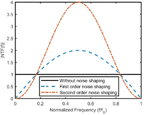
If the NTF has a zero located at DC to form a high-pass filter

To have first-order noise shaping, i.e. the quantization noise is shaped to a frequency far from the modulator bandwidth, the NTF should have a zero located at DC (z = 1) to form a high-pass filter. This requirement can be met using a first-order integrator, with the following transfer function:

𝐻(𝑧) = 1

𝑧 − 1, (2.16)

thus, leading to a 𝑆𝑇𝐹(𝑧) = 𝑧−1 and 𝑁𝑇𝐹(𝑧) = 1 − 𝑧−1. The STF introduces a delay, while NTF implements a first order difference correspondent to a high-pass filter. Considering 𝑧 = 𝑒𝑗2𝜋

𝑓

𝑓𝑆_{, the NTF frequency response is given by:} 𝑁𝑇𝐹(𝑓) = 1 − 𝑒−𝑗2𝜋 𝑓 𝑓𝑆 = sin (𝜋𝑓 𝑓_𝑆) × 2𝑗 × 𝑒 −𝑗2𝜋_𝑓𝑓 𝑆 (2.17)

Adding the noise shaping to (2.12) result in following quantization noise power: 𝑃_𝑄(𝑓) = ∫ 𝑆_𝑄(𝑓)|𝑁𝑇𝐹(𝑓)|2_𝑑𝑓 𝑓𝐵 −𝑓𝐵 = Δ 2_𝜋2 36 1 𝑂𝑆𝑅3 (2.18)

(33)

2.2 Basis of sigma-delta modulation (ΣΔM)

With noise shaping the noise power improves significantly. Now, doubling the OSR results in a 9dB reduction of the quantization noise power.

For higher order noise shaping, is required a higher order loop, and the generic expression of 𝑁𝑇𝐹(𝑧) and quantization noise power is given by:

𝑁𝑇𝐹(𝑧) = (1 − 𝑧−1)𝑁_, _(2.19) and, 𝑃_𝑄(𝑓) = Δ 2_𝜋2𝑁 12(2𝑁 + 1)× 1 𝑂𝑆𝑅2𝑁−1, (2.20)

in which the N is the order of the filter.

Figure 2.11 shows the noise transfer functions for different orders of noise shaping in ΔΣ modulator.

Figure 2.11: Noise transfer function of different orders of noise shaping in ΔΣM

2.2.3 Performance Metrics and Parameters

The noise generated by the circuit and by quantization can have a big impact on ΔΣ modulators performance. The ratio between the output signal power, 𝑃𝑠𝑖𝑔, and the in-band

(34)

noise power without the circuit contributions, 𝑃𝑄, assuming an ideal low-pass filter with

a cut-off frequency equal to the bandwidth of the modulator, and it is given by: 𝑆𝑄𝑁𝑅 = 𝑃𝑠𝑖𝑔

𝑃_𝑄 (2.21)

The maximum SQNR, in dB of a ΔΣ modulator with first order is

𝑆𝑄𝑁𝑅_𝑚𝑎𝑥 = 6.02 × 𝑁 + 1.76 − 5.17 + 30log (𝑂𝑆𝑅) (2.22) Unfortunately, SQNR is not enough for measuring the ADC performance, because it does not take into account the noise caused by the circuit. For that, exists the Signal-to-Noise Ratio, SNR, and Signal-to-Signal-to-Noise-and-Distortion Ratio, SNDR, that also includes the distortion of the circuit.

In Figure 2.12 is shown the relation between SNDR and SNR, and a new parameter, DR, the Dynamic Range. The dynamic is the ratio of the maximum and minimum amplitudes that the converter can process. Both SNDR and SNR increase linearly with amplitude of the input signal until it reached the maximum DR. When the input amplitude gets closer to the maximum, the SNR start increasing slower until it studently drops. The SNDR have a similar behavior but it happens sooner, because of the distortion which is also considered.

(35)

2.3 VCO-based Continuous Time Sigma-Delta ADCs

To evaluate the resolution of an ADC, the Effective Number Of Bits, also known as ENOB is used, and it is given by:

𝐸𝑁𝑂𝐵 ≈𝑆𝑁𝐷𝑅𝑚𝑎𝑥 − 1.76

6.02 (2.23)

FoMs (Figure of Merit) are the most common forms of comparing different circuits. For modulators the Walden FoM [8], that considers bandwidth, BW, power consumption, PC and ENOB and the Schreier FoM [9], that considers SNDR or DR, signal bandwidth

and power consumption are the most common and can be consulted in (2.18), (2.19) and (2.20). 𝐹𝑜𝑀𝑊 = 𝑃_𝐶 2𝐸𝑁𝑂𝐵_{× 2 × 𝐵𝑊}× 1015 [fJ/conv − step] (2.24) 𝐹𝑜𝑀_𝑆1 = 𝑆𝑁𝐷𝑅 + 10 log (𝐵𝑊 𝑃_𝐶 ) [dB] (2.25) 𝐹𝑜𝑀_𝑆2 = 𝐷𝑅 + 10 log (𝐵𝑊 𝑃_𝐶 ) [dB] (2.26)

In the first one, a smaller value is better, while the others a higher value is preferable.

2.3 VCO-based Continuous Time Sigma-Delta ADCs

The principle in this kind of modulators is to count the edges of the wave generated by the VCO, since it produces a signal with a certain frequency depending on the input voltage (Vctrl). Counting the edges within a sampling period will provide an estimation of

the frequency of the VCO’s signal and, consequently, and estimation of the Vctrl as well

[10].

To count the edges of the VCO signal, the phases of all inverters in the ring oscillator are stored in registers, so that, at the end of each sampling period a XOR operation is performed between the current phases of the oscillator and the previous ones, detecting the changes of phase and, consequentially, the edges occurred. Adding the changes detected results in a quantized Vctrl, which corresponds to the input signal.

Figure 2.13 shows the structure of a VCO-based quantizer and the process of counting edges.

(36)

Figure 2.13: VCO-based quantizer: (a) structure; (b) binary sequences (adapted from [10])

In this kind of structure is present a very important feature, the outputs of the XOR gates are barrel-shifted for consecutive phases. What provides an intrinsic Dynamic Element Matching (DEM) within the feedback loop, once each element is used multiple times across the sampling periods while the final output is shifted trough the multiple XOR gates. Therefore, the mismatch between DAC elements is first-order shaped improving the overall resolution of the DAC.

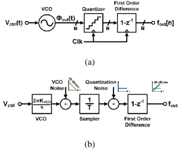
In Figure 2.14 is shown a block diagram and frequency-domain model of the VCO-based quantizer.

Figure 2.14: VCO-based quantizer using the VCO frequency as output: (a) block diagram;

(a) (b)

(a)

(37)

2.3 VCO-based Continuous Time Sigma-Delta ADCs

The quantizer in the block diagram Figure 2.14 a) has as inputs the multiple phases of the multiple ring VCO, so the quantizer block corresponds to the registers that store the sampled phases outputs and the first order difference represents the XOR gates which are responsible for detecting phase changes comparing both registers.

In the second model, frequency-domain, the VCO is simulated by an integrator block with a gain of 2𝜋 × 𝐾_𝑉𝐶𝑂 and the phase noise is added to the output of the integrator block. A sampler with quantization noise added represents the quantizer block. To convert the phase signal of the VCO to a VCO frequency signal, the first order difference is responsible for the operation of differentiation of the current and previous sample, with the transfer function of 1 − 𝑧−1.

So far, the many advantages of VCO-based quantizers have been exposed, although the central block of this kind of quantizer, the VCO, have an inherent problem. It’s voltage to frequency tuning curve is very non-linear and this can lead to harmonic distortion, thus, having a negative impact on the modulator performance, mentioned in [11].

There are some solutions for this problem. The first one is to substitute de VCO for CCO (Current-Controlled Oscillator), since they are much more linear than VCOs. This is due to the fact the current is directly related to the charge time of the inverters in a ring oscillator which is responsible for the oscillation. This solution is studied in [4], comparing both tuning curves of VCO and CCO. The other solution is to put the VCO quantizer in the feedback loop as shown in Figure 2.15, since the presence of high gain filtering reduces the effects of the VCO non-linear tuning curve and phase noise. However, both solutions have problems. The first does not solve the non-linear tuning curve completely and phase noise. The second on needs a high gain filter in the loop, with high power consumption and scaling unfriendly.

Figure 2.15: ΣΔ feedback to suppress VCO linearity and quantization errors (adapted from [10])

(38)

To avoid the non-linear tuning curve of the VCO, a solution, that as become very popular, suggested to use the VCO phase instead of the frequency for the quantized output [12], as shown in Figure 2.16. For that the quantizer compares the phase of the VCO with a phase reference generated by a clock signal. Is no longer required to convert the VCO phase to frequency, so a difference operation is avoided at the quantizer. For this reason, the error resultant of the comparison of phases must be fed back trough a DAC. This way, the quantizer behaves like an integrator with infinite DC gain from the VCO. There is no longer the first order noise shaping, since the first order difference is not present. This way the DAC elements mismatch will have a negative impact on the DAC mismatches, since the generated code no longer depends on counting of edges of the signal of the VCO, the barrel-shifted output is lost, and DEM is lost too. To solve this problem a Dynamic Weight Average (DWA) as to implemented before the DAC elements, increasing general complexity. On the other hand, the impact of non-linearities is very attenuated, since the tuning voltage is confined to a small interval due to the error as input of the VCO.

Figure 2.16: VCO-based CT Σ∆ ADC using the VCO phase as quantized output (adapted from [12])

2.4 Recent approaches to VCO-based CT ΔΣM ADC

In Figure 2.17 is represented an approach suggested in [13] that uses the VCO phase as quantized output. In this case the phase difference between two VCOs, placed in a differential form, is the output of the ADC. Doing this permits the VCOs frequency to be chosen with less restrictions, and, therefore a low frequency can be chosen improving the VCOs phase noise and power consumption. This structure as natural rotation of the DAC selection patterns at the speed of twice the central frequency of the VCOs, resulting in an intrinsic DEM capability of clocked averaging (CLA) [14]. This way the DAC mismatch

(39)

2.4 Recent approaches to VCO-based CT ΔΣM ADC

Figure 2.17: Differential CCO-based CT ΔΣ ADC (adapted from [13])

As the previous work, the ΔΣM present in Figure 2.18 also relies on VCO phase quantized and it also as the VCOs arranged in differential manner, operating very similar and once again suppressing the need for explicit DEM. It also has a extended phase quantizer (PEQ), which not only compares the phases of the two VCOs but also detects which of them is delayed in relation to the other, doubling the overall resolution of the quantizer [15]. The passive loop filters (green) are achieved with elements present in the circuit, namely, the loading effect from the DAC, the input resistor of the DAC (RDAC) and the parasitic effect of the CCO input. This effect is also used as passive integrator for second order noise shaping achievement.

Figure 2.18: CCO-based CT ΔΣM with passive integrator and capacitive feedback (adapted from [16])

Figure 2.19 shows a structure with a very different approach, using a residue cancelling quantizer. The flash ADC quantize the input signal while the VCO quantizer is fed with the difference between the input signal and the flash DAC output of the quantized input (residue). This way, the VCO is going to quantize only the quantization error of the flash ADC, which as voltage swing much smaller than the overall input,

(40)

therefore a smaller interval in the tuning curve of the VCO can be used, thus improving linearity. The overall output is the sum of the input quantized by the flash ADC and the quantization error of this, quantized by the VCO quantizer, resulting in an output free of the quantization noise of the flash ADC, but with the quantization noise of the VCO quantize which is first order shaped. The VCO quantizer uses frequency as quantized output providing intrinsic DEM capability.

Figure 2.19: VCO-based ΔΣM with residue cancelling (adapted from [17])

So far, the circuits presented purpose either VCO frequency or phase as quantized output. The following work, in Figure 2.20, purpose a hybrid idea, using both options.

Figure 2.20: VCO-based ADC with combined frequency and phase feedback (adapted from [18])

The VCO phase goes through a path (blue) and the VCO frequency through other (red) and they are summed for output of the ADC and fed back to the input. With this configuration is possible to achieve an improved linearity (VCO phase quantized characteristic) and intrinsic DEM capability (VCO frequency quantized characteristic), reducing the requirements of the ADC.

(41)

2.5 Comparison of recent works

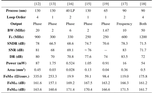
In the Table 2.1 a comparison of the state of the art VCO-based CT ΔΣ modulator ADCs is presented.

Table 2.1: Comparison of state of the art VCO-based CT ΔΣ modulator ADCs

[12] [13] [16] [15] [19] [17] [18]

Process (nm) 130 130 40 LP 130 65 90 90

Loop Order 4 1 2 1 1 2 4

Output Phase Phase Phase Phase Phase Frequency Both

BW (MHz) 20 2 6 2 1.67 10 50 FS (MHz) 900 300 330 250 250 600 1200 SNDR (dB) 78 66.5 68.6 74.7 70.6 78.3 71.5 SNR (dB) 81 68 69.1 ≈ 76 -- 83 71.7 DR (dB) 80 70 70.8 77.6 74 83.5 72 Power (mW) 87 1.75 0.524 1.05 0.91 16 54 Area (mm2₎ _0.45 _0.03 _0.028 _0.13 _0.04 _0.36 _0.5 FoMW (fJ/conv.) 335.0 253.3 19.9 59.1 98.4 119.0 175.8 FoMS1 (dB) 161.6 157.1 169.2 167.5 163.2 166.3 161.2 FoMS2 (dB) 163.6 160.6 171.4 170.4 166.6 171.5 161.7

Looking at Schreier FoM results, [15], [16] and [17], stand out from the other works. [17] is the older reference (2012) of the three and achieved the best result, being the other two much recent (2017). Even though, recent works tend to use phase as quantized output, [17], depicted in Figure 2.19, uses frequency as some older works, achieving great results.

(42)

(43)

3 Current-Controlled Oscillator and Phase

Generator

In this chapter the current-controlled oscillator (CCO) designed and the phase generator are described. The oscillator was developed in Cadence software in CMOS 65nm technology. The way it operates, and results are present in section 3.1. The phase generator was tested with a MATLAB/Simulink® model. The behavior and results achieved are present in section 3.2.

3.1 CCO

For the oscillator there were two important requirements: high linearity in the tuning curve and a large tuning range, in order to achieve the best possible results [20]. For the high linearity, a current-controlled oscillator was chosen since CCOs are known for having a much linear tuning curve than VCOs.

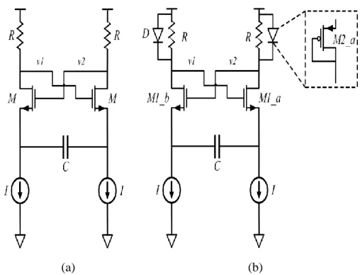
A multiphase oscillator is typically used in VCO-based ΣΔ ADCs. As the number of phases are equal to the number of quantization levels. However, in this architecture, a separated phase generator was used, explained in the next section (3.2). Due to this fact, just a single-phase oscillator was needed. This way was possible to achieve higher gains of frequency in the oscillator [3]. Nevertheless, to achieve high frequencies, a simple circuit must be used. For that reason, a simple relaxation oscillator was chosen, that have, also, the best phase noise performance, theoretically [21], in comparison to ring oscillators. In Figure 3.2(a) it is possible to observe a classic implementation of the circuit. The capacitor acts as an integrator where the capacitor voltage (vC) is the output

(44)

3 Current-Controlled Oscillator and Phase Generator

and the capacitor current (iC) is the input. The rest of the circuit implements the

Schmitt-trigger, shown in Figure 3.1(a), that have as the input the output of the integrator and as output the input of the integrator. The output of the oscillator is the difference between the voltages of the gates of the transistors, v2-v1, by convenience.

(a) (b)

Figure 3.1: Schmitt-trigger: (a) circuit implementation; (b) transfer characteristic (adapted from [3])

(a) (b)

(45)

3.1 CCO

The amplitude of the output signal is 4IR and the oscillator integration constant is I/C. Therefore, its oscillation frequency is:

𝑓₀ = 𝐼 2𝐶(4𝑅𝐼)=

1

8𝑅𝐶 (3.1)

In equation (3.1) it is possible to conclude that it is not possible to control the oscillation frequency with the current I. Therefore, it is a simple oscillator and not a current-controlled oscillator (CCO). In Figure 3.2(b) there is an alternative [22]. By simply adding a PMOS transistor in diode connected configuration in parallel with the resistor it is possible to assume control over the output frequency of the oscillator. This way, the voltage of the resistor is no longer dependent of the current but fixed by the diode that either is on or off. With this approach, the output frequency of the oscillator is given by:

𝑓₀ ≈ 𝐼

𝑉_{𝑠𝑔𝑂𝑁}𝐶 (3.2)

The voltage of the transistor is constant as well as for the capacitance C, and the oscillator frequency is directly proportional to the current I, by the equation (3.2).

The current sources can be implemented by current mirrors. It was extremely important that the linearity of the CCO was less affected as possible. And for that a cascode current mirror in Figure 3.3, was designed.

Figure 3.3: Cascode current mirror

3.1.1 CCO sizing and results

To achieve high frequencies, and to have a wide tuning range, smaller channel lengths in the transistors are preferred, especially in transistors M1_a and M1_b, responsible for the commutation of the Schmitt-trigger, that as to be quick to invert the phase of the wave. A wide channel is also preferred to lower the resistance of the transistors. To the devices

(46)

M2_a and M2_b that implements the diodes in the circuit, the same logic is applied. In the current mirror, the relation applied is 1-to-1, and that is why the dimensions of M3_a, M3_b and M5 are the same, as well as the dimensions of M4_a, M4_b and M6. The transistor M7 is responsible for the bias voltage of the devices M3_a, M3_b and M5. The sizing of all the transistors is shown in Table 3.1. The capacitor C has a capacitance of 200 fF, and the resistors R has a resistance of 5 kΩ. The current Iref is equal to Iin, this is the control current.

Table 3.1: CCO transistor sizing

Device W/L [μm]. Device W/L [μm]

M1_a, M1_b (NMOS) 10/0.06 M4_a, M4_b (NMOS) 1.5/0.18 M2_a, M2_b (PMOS) 20/0.06 M5, M6 (NMOS) 1.5/0.18 M3_a, M3_b (NMOS) 1.5/0.18 M7 (NMOS) 0.15/0.18

The CCO tuning range is shown in Figure 3.4(b). The dashed straight-line next to the tuning curve shows that the oscillator is very linear, especially between 35 μA and 115 μA, with frequencies of 415.6 MHz and 997.8 MHz, respectively. Within this interval, the maximum integral error of linearity is less than 2%, with an average error of 0.45%. The differential error is about 0.17% in average and as a maximum value of 1.1%. This last error is more important due to the small input swing of the oscillator. The central frequency of the CCO is 698.6 MHz at 75 μA of input current. The current-to-frequency gain (KCCO) is about 7.2 THz/A. These results are summarized in Table 3.3.

(47)

3.1 CCO

At high frequencies the output of the oscillator becomes “more sinusoidal” as shown in Figure 3.4(a), and extra circuitry is needed to make it square.

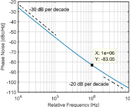
Figure 3.5 shows the phase noise of the implemented CCO and in Table 3.2 some numeric results. It is possible to observe a -30 dB slope correspondent to the flicker noise as well as -20 dB slope at further frequencies caused by the phase noise [23].

Figure 3.5: Phase Noise of the implemented CCO

Table 3.2: Phase Noise of the implemented CCO

Offset Frequency Phase Noise [dBc/Hz]

@100 kHz -55.41

@1 MHz -83.05

@10 MHz -105.90

Table 3.3: CCO results

KCCO [THz/A] f0 [MHz] Linear Range Max. Linearity

Error

Power Consumption [μW]

(48)

3.2 Phase Generator

The great difference in this work to the ones presented in section 2.4 is the way the phases are generated. While in all the approaches studied, a multiphase VCO or CCO where used, in the proposed architecture was decided to use an independent phase generator with a single-phase oscillator. This allows freedom when choosing the architecture of the oscillator.

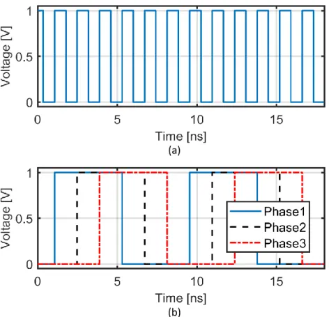
In Figure 3.6(a) it is possible to observe the phase generator architecture studied. The architecture was based on a work about shift-registers used for low jitter multiphase clock generation [24]. It consists in a chain of N D flip-flop (DFF) with the Q output connected to the D input of the next DFF. The oscillator output is fed to the clock input of the DFFs. The last DFF in the chain has its Q output inverted and connected to the D input of the first DFF. This way the first DFF is inverted every N cycles of the oscillator. With this scheme it is possible to have N phases with a delay of an oscillation period of the CCO of each other. Which corresponds to a delay phase of π/N. Each phase as duty cycle of 1/2 and a frequency that is given by:

𝐹𝑟𝑒𝑞𝑢𝑒𝑛𝑐𝑦 𝑝𝑒𝑟 𝑝ℎ𝑎𝑠𝑒 = 1

2𝑁× 𝑅𝑒𝑓. 𝐹𝑟𝑒𝑞𝑢𝑒𝑛𝑐𝑦 (3.3)

Figure 3.7 shows an example of a 3-phase generator results. In Figure 3.7(a) is the reference oscillator waveform and the three phases of the generator are pictured in Figure 3.7(b). Phase1 as its value inverted every 3 periods of the oscillator waveform. Furthermore, the total period of Phase1 is equal to six periods of the reference oscillator wave, what proves that the frequency was divided by 6 (2 × 3 phases). Phase 1, 2 and 3 are delay of one period of the oscillator of each other.

(a) (b)

(49)

3.2 Phase Generator

(a)

(b)

Figure 3.7: 3-phase generator example: (a) Reference oscillator wave; (b) Phases of the generator

Figure 3.6(b) shows the composition of a DFF cell. In each cell there are two latches connected that are enabled alternatively. When the enable signal is low, the first latch is refreshing its output with the input, while the second one is maintaining the output. When the enable signal is high, the first latch is disabled, and the output is maintained, while the second latch is enabled, and the output is refreshed with the output of the first latch. This way the DFF cell is only responsive to the low to high transition of the clock (oscillator wave), meaning that, only the value in this transition is stored in the DFF.

Generating phases with this architecture is also beneficial for the jitter. The jitter from oscillator is transferred to the DFF chain without improvement. However, the jitter added is due to noise jitter and mismatch jitter, and there is no accumulation from one cell to the next one. This happens because each DFF output only acts as an enabler for the next one, being the CCO responsible for the timing [24].

(50)

(51)

4 Single phase CCO-based ΣΔM with

separated phase generator

In this chapter a description of the proposed ΣΔ modulator architecture is presented. For the implementation of the structure, a MATLAB/Simulink® model was developed for all tests carried out. The data gathered from the CCO simulations in Spectre environment was used to model the oscillator in this architecture model. The main features of the proposed architecture are described in section 4.1 and the results of the simulations are present in section 4.2.

4.1 Proposed Architecture Characteristics

The proposed ΣΔ modulator architecture presented in Figure 4.1 was based on a K. Lee, Y. Yoon, and N. Sun work [4], with some variations. First, the multiple phases were not generated in the oscillator, but with a completely independent robust phase generator block [24]. This provided some freedom for the design of the oscillator with a single output phase. It was also opted for a second order loop with a low-pass filter and two different DAC blocks for a second order noise shaping.

The oscillators were still arranged in pseudo-differential manner as the original work [4]. This way, the output was the difference of phase between the two CCOs, and there was no need for the central frequency of the CCO being fixed to a fraction of the sampling frequency. However, the central frequency could not be set too low in this architecture as has been clarified in the Phase Generator (3.2) section. The pseudo-differential arrangement of the oscillators also reduced the even order distortions.

(52)

4 Single phase CCO-based ΣΔM with separated phase generator

Figure 4.1: Proposed Architecture

The second order loop (40dB per decade slope can be observed in Figure 4.2.) was achieved with the oscillators used as integrators and active low-pass filters implementing a moderate loop gain (20 dB). This way, it was possible to achieve a smaller input swing in the CCOs, thus reducing the linearity issues introduced by the oscillator.

As for the number of phases in the phase generator, there was a tradeoff. With a higher number of phases, it was possible to have more quantization levels. However, the current-to-frequency gain of the CCOs (KCCO) dropped drastically, as detailed in section

(53)

4.1 Proposed Architecture Characteristics

4.1.1 DAC selection pattern

In Figure 4.3(a) is visible a spectrum result of a simulation of the MATLAB®_{model in}

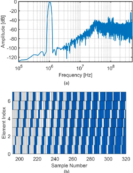
which a 3-bit quantizer (7-phase oscillator) was implemented. In this simulation, only the quantization noise is present because the feedback DAC components are ideal and have no mismatch problems or any kind of noise. However, considering process, voltage and temperature (PVT) variations that happen in the physical world and affects the components. Thus, leading to mismatches that degrade the linearity of the overall architecture. In Figure 4.3(b) are visible results of a classic 3-bit thermometer-coded DAC in a second-order ΣΔ ADC simulation. A lot of tones appear within the signal bandwidth, due to the data deterministic behavior of the DAC selection pattern. The tones generated by this selection pattern are added in the two summing nodes and have a negative impact on the SNDR. In this case the SNDR dropped about 13 dB from the ideal case.

(a)

(b)

Figure 4.3: Thermometer DAC with 1% mismatch: (a) Output spectrum; (b) DAC cell selection pattern

(54)

To overcome the thermometer-coded DAC deterministic selection pattern, explicit dynamic element matching (DEM) can be used. So that, the DAC selection pattern becomes more random and less deterministic. Nevertheless, the proposed structure generates a natural rotation of selection of the DAC elements, visible in Figure 4.4(b) with a speed of approximately twice of the CCO center frequency [4]. This feature implements DEM scheme of clock averaging (CLA), thus eliminating the need for explicit DEM blocks. The CLA moves the influence of the DACs mismatches away from signal bandwidth, reducing the effects on the SNDR. This effect can be observed in Figure 4.5, where a 25% mismatch was tested to really highlight the modulation. The simulation results of this case, in Figure 4.4(a), prove that with mismatches of 1% in DAC elements, SNDR drops only 3 dB from the ideal case, instead of 13 dB in the previous example.

(a)

(b)

Figure 4.4: Natural rotative DAC with 1% mismatch: (a) Output spectrum; (b) DAC cell selection pattern

(55)

4.2 Full architecture results

Figure 4.5: Natural rotative DAC with 25% mismatch: Output spectrum

4.2 Full architecture results

Three models of the proposed architecture were developed in MATLAB/Simulink®_.

Between them, the only visible difference was the number of phases (7, 15 and 25) and DAC elements besides different parametrizations. Implementing three different resolutions for the ADC. For each resolution several tests were carried out:

• With a linear approximation of the oscillator:

• Active low-pass filter (20 dB) and 0% DAC mismatch; • Active low-pass filter (20 dB) and 1% DAC mismatch; • Passive low-pass filter and 0% DAC mismatch;

• CCO tuning range seven times smaller than the implemented, active low-pass filter (20 dB) and 0% DAC mismatch;

• With a polynomial approximation of the oscillator;

• Active low-pass filter (20 dB) and 0% DAC mismatch; • Active low-pass filter (20 dB) and 1% DAC mismatch.

A sampling frequency of 1 GHz was considered in every test, as well as bandwidth of 5 MHz, which corresponds to an OSR of 100. The maximum input signal amplitude in the simulations was 160 μA peak-to-peak in differential mode, equivalent to 80 μA to each CCO input. The input signal frequency was about 1 MHz.

The CCO is modeled with an ideal VCO block from Simulink® and a Schmitt trigger to have square wave. The first order low-pass filter has time constant of 50 μs.

(56)

In Table 4.1 is present a description of the simulations made for each model implemented.

Table 4.1: Description of simulation tests

Test CCO approx. DAC Mismatch [%] Filter Gain [dB]

1 (Ideal) Linear 0 20

2 Linear 1 20

3 Linear 0 0

4 Linear (-tuning range) 0 20

5 Polynomial (6th_order) ₀ ₂₀

6 (C. Real) Polynomial (6th_order) ₁ ₂₀

The first test, Test 1, was considered the test with ideal conditions and where the best results were achieved. The last test, Test 6, was the test with the closest conditions to a real circuit implementation, performed in this study.

4.2.1 7-phase ADC (3-bit)

In Figure 4.6 it is possible to observe the output spectrum of what is considered an ideal simulation. There was no mismatch in DAC elements, the CCO was completely linear with a KCCO of 7.2 THz/A which corresponds to KCCO per phase of 514.29 GHz/A. The

low-pass filter had gain of 20 dB. These were the conditions, in which the best results were achieved. In the spectrum is clearly visible the peak in the input signal frequency (about 1 MHz). as well as 40 dB per decade slope. For this simulation, the SNR value was about 81.27 dB and the SNDR value of 80.79 dB.

The second simulation only a 1% mismatch in the DAC elements was introduced, maintaining a linear CCO, and 20 dB of gain in the low-pass filter. In these conditions, as expected, the SNR and SNDR values dropped to 77.75 dB and 76.92 dB, respectively. In order to observe the influence of the gain in the filter, the third simulation had no gain (0 dB), maintaining the other ideal conditions, linear CCO and 0% mismatch in DAC elements. The output spectrum of this simulation is present in Figure 4.7 and there are some noticeable differences from the ideal case. First, there is a much higher noise floor at around -110 dB as opposed to the -130 dB of the ideal case. Second, the 40 dB per decade slope is lost and is closer to 20 dB per decade. For these reasons, the SNR and SNDR values dropped drastically to 59.51 dB and 58.84 dB, respectively.

(57)

Figure 4.6: Output spectrum of ADC with 7-phase generator (ideal test)

(58)

A hypothetical CCO with a smaller but linear tuning range was also tested. With a reference KCCO (1 THz/A) about seven times smaller than the CCO implemented and

maintaining all the ideal conditions of the first test, the architecture achieved a SNR value of 64.67 dB and a SNDR value of 63.83 dB.

The effect of the non-linearities of the CCO tuning curve were also studied in the fifth simulation with results of 76.51 dB and 75.91 dB, respectively, SNR and SNDR.

At last, a simulation with filter gain of 20 dB, a DAC mismatch of 1% and non-linear KCCO was carried out. This was the simulation that was, theoretically, closer to a

real implementation. Aside from the filter gain, all the other negative effects in previous simulations were considered in this simulation. In Figure 4.9 it is possible to observe the output spectrum of this simulation. The main difference to the ideal one (Figure 4.6) is in the lower frequencies due to an offset in the output code caused by the effects of non-linearities in the CCO tuning curve. Figure 4.8 shows this offset, even though, all the scale of codes is used, the lower code values were less selected, causing a DC offset. The dynamic range is shown in Figure 4.10, with a top SNR of 74.19 dB and SNDR of 73.74 dB.

Figure 4.8: Output code of ADC with 7-phase generator (1% DAC mismatch, non-linear KCCO)

(59)

Figure 4.9: Output spectrum of ADC with 7-phase generator (1% DAC mismatch, non-linear KCCO)

Figure 4.10: Dynamic range of ADC with 7-phase generator (1% DAC mismatch, non-linear KCCO)

(60)

The parameters used in the simulations described above are listed in Table 4.2. The DAC1 element current in the table corresponds to the current of each cell of the DAC array listed as DAC1 in Figure 4.1. The DAC2 element current was three times bigger than the current of the DAC1 in every test. The reference KCCO is relative to the relaxation

oscillator. The gain per phase of the CCO is 14 times smaller (2×7 phases).

Table 4.2: 7-phase ADC parameters and SNR results

Test Reference KCCO

[THz/A].

Mismatch [%]

Filter Gain [dB]

DAC1 element current [μA] SNR [dB] 1 7.2 (linear) 0 20 4.25 81.27 2 7.2 (linear) 1 20 4.25 77.75 3 7.2 (linear) 0 0 3.75 59.51 4 1 (linear) 0 20 4.25 64.67 5 7.2 (non-linear) 0 20 4.75 76.51 6 7 .2 (non-linear) 1 20 4.75 74.19

4.2.2 15-phase ADC (4-bit)

The tests made for the 7-phase ADC were repeated for 15-phase and 25-phase ADCs. First, the ideal test with a CCO with a linear KCCO of 7.2 THz/A equivalent to KCCO per

phase of 240 GHz/A. A 20 dB gain in the low-pass filter and 0% mismatch in the DAC elements were also considered. Figure 4.11. shows the output spectrum of the ADC in this simulation. The result was similar to the 7-phase correspondent test, both visually and quantitively, with a SNR and SNDR values of 80.46 dB and 79 dB, respectively.

In the second test, with 1% mismatch in the DAC elements, a linear CCO, and a filter gain of 20 dB, the SNR value dropped to 78.62 dB, as the SNDR to 77.65 dB.

The third simulation, with a passive filter, linear CCO tuning curve and without mismatch in the DAC elements, achieved a SNR value of 59 dB and a SNDR value of 58.53 dB. In Figure 4.12. it is possible to understand the reasons of such a high drop. The 40 dB per decade slope characteristic of the second order noise shaping was lost, and the noise floor was also higher than in the ideal case.

With a CCO with a linear reference KCCO of 1 THz/A and the conditions of the first

test, the model achieved values of 62.13 dB for the SNR and 61.63 dB for the SNDR. Considering a non-linear CCO tuning curve and the rest of the ideal conditions the

(61)

Figure 4.11: Output spectrum of ADC with 15-phase generator (ideal test)

(62)

The final simulation was the closest to an actual circuit implementation, with all the effects considered, 1% mismatch in the DAC elements, non-linear CCO tuning curve and 20 dB of gain filter. Figure 4.14 shows the output spectrum of the ADC. As in the 7-phase example, the lower frequencies had a high power relative to the noise floor. This effect was caused by the non-linear response of the CCO tuning curve that dislocated the output, generating a DC offset. This offset is clearly observable in Figure 4.13. The output codes used were between 2 to 14 for a maximum amplitude input, in a 0 to 15 scale. This led to a maximum SNR value of 77.21 dB and a SNDR value of 76.35 dB, as shown in dynamic range plot (Figure 4.15).

The parameters used in the simulations described above are listed in Table 4.3. The DAC1 element current in the table corresponds to the current of each cell of the DAC array listed as DAC1 in Figure 4.1. The DAC2 element current is three times bigger than the current of the DAC1 in every test. The reference KCCO is relative to the relaxation

oscillator. The gain per phase of the CCO is 30 times smaller (2×15 phases).

Figure 4.13: Output code of ADC with 15-phase generator (1% DAC mismatch, non-linear KCCO)

(63)

Figure 4.14: Output spectrum of ADC with 15-phase generator (1% DAC mismatch, non-linear KCCO)

Figure 4.15: Dynamic range of ADC with 15-phase generator (1% DAC mismatch, non-linear KCCO)