Market neutral volatility: a different approach to the S&P 500 options market efficiency

(1)

MARKET NEUTRAL VOLATILITY: A DIFFERENT APPROACH TO

THE S&P 500 OPTIONS MARKET EFFICIENCY

João Pedro Bento Ruas

Thesis submitted as partial requirement for obtaining the degree of

Master in Finance

Supervisor:

Prof. Doutor José Dias Curto, Assistant Professor, ISCTE - IUL, Department of Quantitative Methods

(2)

Abstract

Under the efficient market hypothesis, an options price’s implied volatility should be the best possible forecast of the future realized volatility of the underlying asset. In spite of this theoretical proposition, a vast number of studies in the financial literature found that implied volatility is a biased estimator of the future realized volatility. These findings suggest that we are either in the presence of an inefficient market or that econometric models fail on that purpose.

In this thesis, by introducing the concept of Market Neutral Volatility and the derivation of a theoretical model, we show what in fact the implied volatility forecasts and we prove that the S&P 500 options market is efficient. This property of the S&P 500 options market assures that the implied volatility cannot be a biased forecast of its future realized volatility. Thus, we conclude that the bias of the implied volatility estimator is due to the inadequacy of the commonly used econometric approaches.

Abstract

Sob a hipótese de eficiência dos mercados, a volatilidade implícita de uma opção deve ser a melhor previsão possível da futura volatilidade realizada do activo subjacente. Apesar deste argumento teórico, um vasto número de estudos realizados na literatura financeira, concluem que a volatilidade implícita é um estimador enviesado da volatilidade realizada futura. Estes resultados sugerem que, ou estamos na presença de um mercado ineficiente, ou que a metodologia econométrica utilizada é inadequada. Através da introdução do conceito de Market Neutral Volatility e da derivação de um modelo teórico, é demonstrado, o que na realidade a volatilidade implícita estima, e provamos que o mercado de opções sobre o S&P 500 é eficiente. A eficiência do mercado de opções sobre o S&P 500, garante que a volatilidade implícita desse mercado não pode ser um estimador enviesado da volatilidade realizada futura. Estes resultados permitem concluir que o problema da obtenção de estimativas enviesadas, deverá resultar do uso de metodologias econométricas inadequadas.

JEL Classification Codes: G10; G14

(3)

Executive Summary

Under the efficient market hypothesis, an option price’s implied volatility should be the best possible forecast of the future realized volatility of the underlying asset. In spite of this theoretical proposition, a vast number of studies in the financial literature found that implied volatility is a biased estimator of the future realized volatility. These findings suggest that we are either in the presence of an inefficient market or that the econometric models fail on that purpose. In this thesis we address this problem and prove that the bias found in numerous studies comes from the use of an inadequate econometric approach.

To demonstrate this we introduce the concept of Market Neutral Volatility and derived a theoretical model to show the relationship between the Market Neutral Volatility, the VIX and the future realized volatility.

Based on that relation, we show that in the long run an agent cannot achieve abnormal returns trading the S&P 500 options market. This implies that the VIX is correctly forecasting the future realized volatility of the S&P 500 (measured by the Market Neutral Volatility and not by the commonly used indicator described by the equation 2.12) leading us to conclude that the S&P 500 options market is, in fact, efficient. This also shows that no other source to forecast the future realized volatility will outperform the forecast given directly by the market through the VIX.

(4)

Acknowledgments

I wish to thank to all of those who contributed either directly or indirectly to this work.

To my supervisor Professor José Dias Curto, for his monitoring, suggestions and for giving me total freedom of thought and action.

To Professor João Pedro Nunes for his critical reading of the thesis and suggestions.

To my family who always supported me in this challenge and in a very special way to my grandparents, mother and sister for their unconditional support.

To my friend Isabel Mendes for her help and support throughout this project.

(5)

Index

1. Introduction ...6

2. The Market Neutral Volatility ...8

2.1 Model Assumptions ...8

2.2 Market Neutral Volatility definition...10

2.3 Realized Volatility...10

2.4 The relationship between realized volatility and the MNV...11

2.5 The MNV and the VIX...13

3. Empirical Analyses ...13

3.1 Data ...13

3.2 The S&P 500 index ...14

3.3 The VIX...14

3.4 Descriptive statistics ...17

3.5 VIX Unit Root...18

3.6 The relationship between the VIX and the S&P 500...19

3.7 Testing the market efficiency in the S&P 500 options market...19

4. Conclusion...21

References...23

(6)

1. Introduction

The implied volatility (hereafter IV) in an option’s price can be seen as the market’s forecast of the future volatility for the underlying asset over the option remaining life. Under the rational expectations assumption that the market uses all the available information and the market’s efficiency hypothesis, the IV should be the best possible forecast of the future volatility given the currently available information. If this is not true, the option pricing theory tells us that if an option fails to embody optimal forecasts of the underlying asset’s future volatility, a profitable trading strategy would be available and its implementation would push the option price to the best possible forecast of future volatility.

Despite these theoretical arguments, a large number of empirical financial studies revealed several problems when the option prices’ IV is used as the estimator of the underlying asset’s future volatility. A common test to assess the forecasting ability of the option’s prices IV, consists in running the following regression:

τ τ τ τ τ =α +β t +γ t− +εt+ t IV HV RV_, _, _, (1.1)

where RVt,τ is the realized volatility of the underlying asset over the period t to t+τ, IVt,τ

is the implied volatility at time t with time to maturity τ, HVt-τ,τ is the historical

volatility over the preceding period t-τ to t, and εt+τ is a zero mean error uncorrelated

with the forecasting variables.

Three hypotheses are typically tested in the literature concerning this regression. First, IV is informative about future volatility only if the estimate for β is significantly greater than zero. Second, IV is an unbiased estimator if the joint hypothesis of α equal to zero and β equal to 1 is not rejected. Third, IV is informational efficient if no other variable (e.g. historical volatility) is statistically significant, that is, γ is equal to zero.

Most of the studies in the literature find evidence that IV forecasts of future volatility are informative1 but biased with β greater than zero but lower than one and α different from zero (Feinstein (1989) and Ederington and Guan (1999, 2002). The evidence on

1_{An exception to this evidence can be found in Canina and Figlewsky (1993) that find weak or no} correlation between IV and future realized volatility.

(7)

informational efficiency is mixed. Day and Lewis (1992), Ederington and Guan (1999, 2002) and Martens and Zein (2002) find evidence that ARCH models and average historical volatility add incremental information. On the other hand, Blair, Poon and Taylor (2001), Christensen and Prabhala (1998), Fleming (1998), Fleming, Ostdiek and Whaley (1995), Hol and Koopman (2001) and Szakmary, Ors and Davidson (2002) find that IV dominates volatility forecasts.

The bias of the IV estimator that is consistently found in the financial literature means that options might be over (this is the conclusion in a large number of studies) or under priced which can only be the result of an incorrect option price model2, an inefficient market under study or an inadequate econometric approach (this can be due to the proxy for the realized volatility, for example).

If the first two reasons mentioned above were to be true, this would have major implications on the foundations of modern finance. Thus, the third reason seems to be the more plausible one as we will see next.

As in general the VIX (see section 3.3 for VIX details) is used to quantify the IV in the S&P 500 options market, we can exclude that bias comes from an incorrect option pricing model, due to the fact that VIX calculation does not rely on any option price model; it is a model free variable. Moreover, the use of VIX allows us to use an estimate of future volatility that is directly traded in the options market, as in 2004 the Chicago Board Options Exchange introduced exchange-traded VIX future contracts which made the volatility a financial asset directly tradable.

Thus, the main purpose of this thesis is answer to the following question: which one of

the two remaining potential sources of bias, an inefficient S&P 500 options market or the inadequacy of econometric methods, is responsible for the results found on the majority of the empirical literature? To achieve this we introduce the concept of Market Neutral Volatility (hereafter MNV) and derive a theoretical model that shows the relationship between this concept and the realized volatility. By using this model we show that the VIX is directly forecasting the Market Neutral Volatility and not the realized volatility as it is computed in most of financial studies (see equation 2.12). Thus, we show that MNV is the correct proxy for the realized volatility.

2

(8)

Using the theoretical model presented in this thesis we find empirical evidence of the S&P 500 options market efficiency. This finding points out the misapplication of the econometric methods as the main source of bias in the IV forecasts of future volatility. The empirical findings of this thesis also allows us to conclude that given a correct estimation of future volatility (being this estimation given directly by the market, like in the VIX case) the Black-Scholes formula correctly prices an at the money S&P 500 option.

The remainder of this paper is organized as follows: Section 2 introduces the concept of Market Neutral Volatility and a theoretical model is derived to show the relationship of Market Neutral Volatility and realized volatility. Section 3 contains the data description and the empirical analyses related with the application of section 2 theoretical results. Section 4 summarizes our concluding remarks.

2. The Market Neutral Volatility

2.1 Model Assumptions

Let is assumed the following model assumptions for a tradable stock index:

• Pt is the market price of the stock index at the closure of day t.

• Vt+1 = Pt+1-Pt

• rt+1 =

(

Pt+1−Pt

)

/Pt .

• rt+1 ~ N(0; σt+1), being σt+1 the realized market volatility at t+1 not know in t.

• t+1 minus t equals one trading day.

• risk free rate (r) and dividend yield (q) equal to 0%.

• tradable european calls and puts with one day time to maturity available right after the close of the market at t.

• Straddle (gt) = callt ATM3 + putt ATM.

3

(9)

According to the Black-Scholes model (Black and Scholes, 1973) the value of a european call and put is given by the following formulas:

) ( ) ( 2 ) ( 1 ) ( d Ke d e S callt = t qT t Φ − rT t Φ − − − − (2.1) and ) ( ) ( 2 ) ( 1 ) ( d Ke d e S putt =− t qT t Φ − + rT t Φ − − − − − (2.2) with ) ( ) )( 2 / ( ) / ln( 2 1 t T t T q r K S d t − − + − + =

σ

(2.3) ) ( 1 2 d T t d = −σ − _(2.4) and

( )

x

∫

xe u du ∞ − − = Φ 2/2 2 1

π

. (2.5)

The stock price, strike, risk free rate, dividend yield, time to maturity and volatility are denoted by, S, K, r, q, (T-t),σ, respectively.

By put-call parity ) ( ) (T t rT t q t t t put S e Ke call − = − − − − − _(2.6)

which with q = 0%, r = 0% and S = K becomes

. t t put

call = _(2.7)

Assuming the rationality of the agents, the price at which an agent would be willing to sell a straddle at the end of t with the information of the closure of t+1 becomes

(10)

gt=[│Vt+1│;+∞[ (2.8)

and likewise the price at which an agent would be willing to buy a straddle in the same period

gt = [0;│Vt+1│] (2.9)

it follows as the only possible equilibrium price

gtE =│Vt+1│. (2.10)

2.2 Market Neutral Volatility definition

Let Market Neutral Volatility be defined as the IV in t such that

gtE(MNVt) =│Vt+1│. (2.11)

That is, MNV is defined as the IV at the end of t that, with the information of the closure of t+1, makes the value of a straddle at t equal to the absolute change in the price of the stock index from the end of t to the closure of t+1.

2.3 Realized Volatility

Let the annualized realized volatility be defined as:

) ( 1 1 1 t T Pt P P e_t t t − − = + +

σ

(2.12)

This method of calculating market volatility comes from the notion that the payout of a european option at expiration only depends on the difference between Pt+1 and Pt and

(11)

not on the prices observed in the market between that interval. This way of measuring volatility also takes inspiration on former works found in the literature.

Figlewski (1997) suggests that taking deviations around zero instead of the sample mean typically increases volatility forecast accuracy. Ding, Granger and Engle (1993) suggest measuring volatility directly from absolute returns. Andersen and Bollerslev (1998) refer to daily realized volatility as the sum of intraday squared returns.

2.4 The relationship between realized volatility and the MNV

If we have the market value of an european call ATM we can get the IV of that option using the Black-Scholes formula. Even though a directly close formula to calculate the IV cannot be derived from equation (2.1), a good approximation is given by Brenner and Subrahmanyam (1988) in the following way4:

t P callt t T i ) ( 2 − ≈

π

σ

(2.13)

Using equation (2.13) and replacing σi by the MNV defined in Section 2.2 we get

Pt call t T MNV E t t ) ( 2 − =

π

(2.14) Using equation (2.10) 1 + = + t E t E t put V call (2.15) and equation (2.7) E t E t put call = (2.16) we get 4

(12)

2 1 + = t E t V call . (2.17)

Replacing equation (2.17) in equation (2.14)

Pt V t T MNV_t t 2 ) ( 2 +1 − =

π

(2.18) Pt V t T MNV_t t 1 2 1 ) ( 2 + − =

π

(2.19)

After some algebra, equation (2.12) can be written as

) ( . 1 1 t T e P V t t t − = ₊ +

_σ

(2.20)

Replacing equation (2.20) in equation (2.19) we get

) ( . . 2 1 ) ( 2 1 T t e t T MNV_t _t − − =

π

σ

₊ (2.21)

and after some algebra5

1 2 2 1 + ⋅ = t t e MNV π σ . (2.22)

Based on this result we can conclude that the Market Neutral Volatility (MNV) in time t is approximately equal to 1.25 times the realized volatility of t+1.

5_{We are assuming that both options and the daily returns of the stock index are annualized with the same} number of days. If they are annualized using a different factor, then equation (2.22) becomes

c c r r t t t T t T e MNV − − ⋅ ⋅ ≈ 2 ₊1 2 1

σ

π

σ

, with r and c referring to the factor used on the daily returns and options respectively.

(13)

2.5 The MNV and the VIX

Since the VIX is an ex-ante observable measure of the IV in the S&P 500 options market and the MNV is an IV in an option price calculated ex-post, we can postulate the argument that the VIX is directly estimating the MNV. That is:

∑

= = = T t t T t t VIX T MNV T 1 1 1 1 (2.23)

which using equation (2.22) is equivalent to

∑

= + = ⋅ = T t t T t t e T VIX T 1 1 1 2 2 1 1 1 σ π . (2.24)

3. Empirical Analysis

3.1 Data

In this thesis we used the closing values of the VIX and S&P 500 from the period September 23, 2003 to August 28, 2009, totalling 1495 daily observations. Three reasons lead us to the choice of this period. First, the methodology and the availability of data as we have it today on VIX, were only introduced on September 2003. Second, only in 2004 the VIX futures were introduced which would have contributed to the elimination of any possible market inefficiencies prior to that date. Third, in this period we have very low volatility periods and also extremely high volatility periods (not seen since the 1987 stock market crash) which allow us to make robust assessments about the possibility of options market efficiency since the market was analysed in a large range of values.

(14)

3.2 The S&P 500 index

The S&P 500 index is a price index of stock prices of the 500 largest companies actively traded and quoted in the United States.

In Figure 1 we have the evolution of the daily closing prices of the S&P 500 from September 2003 to August 2009. We can clearly see the bull market rally that lasted from 2003 until the middle of 2007 and the sharp decline started then until the beginning of 2009 (the market lost more than 50% of its value in this period), originated by the global financial crisis.

Figure 1: Evolution of S&P 500 daily closing prices

600 700 800 900 1000 1100 1200 1300 1400 1500 1600 2004 2005 2006 2007 2008 2009 S P 5 0 0 3.3 The VIX

“VIX measures 30-day expected volatility of the S&P 500 Index.” (Chicago Board Options Exchange (2009)).

In 2003, the Chicago Board Options Exchange (CBOE) updated the VIX to reflect a new way to measure expected volatility. The new VIX is based on the S&P 500 Index

(15)

and estimates expected volatility by averaging the weighted prices of SPX puts and calls over a wide range of strike prices. By supplying a script for replicating volatility exposure with a portfolio of SPX options, this new methodology transformed VIX from an abstract concept into a practical standard for trading and hedging volatility.

The VIX is calculated from the transaction values of all calls and puts on the S&P 500 that have a bid price different from zero using the following formula6

, 1 1 ) ( 2 2 0 2 2       − − ∆ =

_∑

K F T K Q e K K T i RT i i i σ (3.1) where

• Pt is the market price of the stock index at the closure of day t.

• σ = VIX/100.

• T = Time to expiration in calendar days. The VIX uses 365 days in all its calculations.

• F = Forward index level derived from index option prices.

• K0 = First strike below the forward index level, F.

• Ki = Strike price of ith out-of-the-money option; a call if Ki>K0 and a put if Ki< K0; both put and call if Ki=K0.

• ∆Ki = Interval between strike prices – half the difference between the strike on

either side of Ki:

2 1 1 − + − = ∆ Ki Ki Ki (3.2)

• R = Risk-free interest rate to expiration.

• Q (Ki) = The midpoint of the bid-ask spread for each option with strike Ki.

6

(16)

The formula in equation (3.1) only uses out-of-the-money options. Thus, Q(Ki,T) represents the call option price when Ki > F and the put option price when Ki < F. When Ki = K0, CBOE uses the average of the call and put option prices at this strike as the input for Q(K0,T). Since K0 ≤ F, the average at K0 implies that the CBOE uses one unit of the in-the-money call at K0. The last term in equation (3.1) represents the adjustment term via the put-call parity to convert this in-the-money call into an out-of-money put.

The calculation involves all available call options at strikes greater than F and all put options at strikes lower than F. The bids of these options must be strictly positive to be included. When at the boundary of the available options, the definition for the interval

∆K modifies as follows: ∆K for the lowest strike is the difference between the lowest

strike and the next higher strike. Likewise, ∆K for the highest strike is the difference between the highest strike and the next lower strike.

To determine the forward index level F, CBOE chooses the pair of put and call options whose prices are the closest to each other. Then, the forward price is derived via the put-call parity relation.

The CBOE uses equation (3.1) to calculate σ2 at two of the shortest maturities of the available options, T1 and T2. Then, the CBOE linearly interpolates between the two σ2 to obtain a σ2 at 30-day maturity. The VIX represents the annualized percentage of this 30-day σ,         − − + − − = 1 2 1 1 2 2 30 30 30 365 100 2 22 2 1 1 T T T T T T N N N T N N N T VIX σ σ (3.3)

where NT1 and NT2 denote the number of actual days to expirations for the two

maturities. When the shortest maturity falls within eight days, the CBOE switches to another maturity to avoid microstructure effects at very short option maturities.

(17)

In Figure 2 we have the evolution of the VIX daily closing values from September 2003 to August 2009. From 2003 to the beginning of 2007 we see a steady decline in the VIX from values around 20 to values around 10. In the beginning of 2007 we start to see a rapid increase in the VIX until the middle of 2008 and then an explosive move up achieving values above 80 at the end of 2008. Since then, with the global response to the financial crisis, VIX values return to values in the middle 20’s.

Figure 2: Evolution of VIX daily closing values

0 10 20 30 40 50 60 70 80 90 2004 2005 2006 2007 2008 2009 V I X 3.4 Descriptive statistics

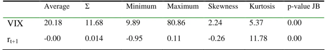
In Table 1 we present the descriptive statistics of the VIX and the daily returns of the S&P 500. The rt+1 variable is the daily return of the S&P 500 calculated as

(

t t

)

t

t P P P

(18)

It is evident from Table 1 the large amplitude in the VIX values (ranging from 9 to 80) with the average near the minimum value of the range. To assess if any of the variables follow a normal distribution we run the JB test on both of them. We reject normality on both with p-values of 0.00 with the distribution of the daily returns of the S&P 500 skewed to the left and leptokurtic which is consistent with the literature.

Table: 1 VIX and daily returns of the S&P 500 descriptive statistics

Average Σ Minimum Maximum Skewness Kurtosis p-value JB

VIX 20.18 11.68 9.89 80.86 2.24 5.37 0.00

rt+1 -0.00 0.014 -0.95 0.11 -0.26 11.78 0.00

3.5 VIX Unit Root

Although the VIX is not directly tradable in the market, the existence of VIX futures7 contracts and options on the VIX, should lead to E(VIXt+1) = VIXt. To verify this

hypothesis we tested the existence of a unit root in the VIX time series. For that we performed the ADF test on the VIX time series and the results are presented in Table 2.

Since we cannot reject the existence of a unit root (φ1= 1) at the 1% significance level in

all three models tested the results obtained confirm that E(VIXt+1) = VIXt,.

Table 2: ADF test on VIX time series

Model (φ1-1) ADF test Asymptotic p-value

(1-L)VIXt = (φ1-1)*VIXt-1+εt -0.00261745 -1.27053 0.1883 (1-L)VIXt =b0+(φ1-1)*VIXt-1+εt -0.0109104 -2.65105 0.08281 (1-L)VIXt =b0+b1*t(φ1-1)*VIXt-1+εt -0.0181447 -3.48271 0.04119

7_{Brenner, Shu e Zhang (2007) estimates that the correlation between the VIX and the 30-day VIX} Futures to be 0.8140.

(19)

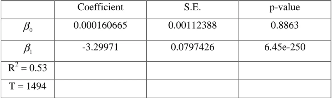
3.6 The relationship between the VIX and the S&P 500

To analyze the relationship between the VIX and S&P 500 at time t we run a regression of the daily rate of change of the VIX (rVIXt) over the daily returns of the S&P 500

(rSP500t) in the following form:

t t

t rSP

rVIX =β₀ +β₁ 500 +ε (3.4) The results obtained are presented in Table 3. Only β1 is significantly different from 0

and takes a negative value pointing to an inverse relationship between the VIX and the S&P 500.

Table 3: The relationship between the VIX and the S&P 500

Coefficient S.E. p-value

0 β 0.000160665 0.00112388 0.8863 1

β

-3.29971 0.0797426 6.45e-250 R2 = 0.53 T = 1494

3.7 Testing the market efficiency in the S&P 500 options market

In sections 3.5 and 3.6 we showed two important results. First, for the same period t we have a direct relationship between the change in VIX values and the change in S&P 500 prices. Second, the best estimate for the value of the VIX at t+1 is its value at t. These findings assure us that the VIX market is efficient. These findings also allow us to conclude that: if E(VIXt+1) ≠ VIXt (in opposition to what was shown in section 3.5) and

having VIX value changes at t directly related with S&P price changes at t, some part of the biased forecasts of the future realized volatility given by the IV found in the literature, could be explained by the fact that the VIX in period t was already a biased forecast estimator of VIX for t+1. As we showed that E(VIXt+1) ≠ VIXt we can discard

(20)

Given the definition introduced in section 2.2, the MNV is the ex-post IV that assures the efficiency in an options market. By using the definition of the realized volatility given by equation (2.12) and the model derived in section 2, we showed that the relationship between MNV and future realized volatility is illustrated by the equation (2.22). Since MNV is an ex-post IV and being the VIX an ex-ante IV we postulate that VIX is in fact the market forecast for the MNV. Thus, to prove empirically that the S&P 500 option’s market is efficient we need to show that equation (2.24) holds.

We then have to test the following hypothesis:

0 :

0 VIX − MNV =

H µ µ

based on the sample means difference:

0 ˆ 2 2 1 1 1 1 1 1 = ⋅ −

∑

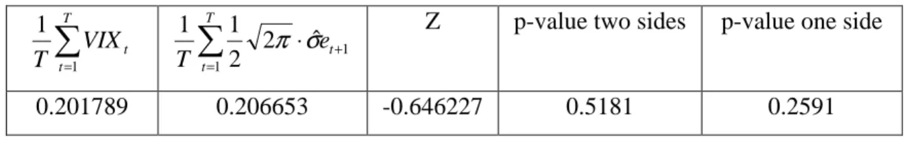
= + = T t t T t t e T VIX T π σ . (3.5)

To assess the validity of this hypothesis, we performed a two independent samples t test which allows to compare the means of two variables8. The results are shown in Table 4.

As the results presented in Table 4 suggest, we cannot reject the null hypotheses that both means are equal with high confidence level, allowing us to confirm that equation (2.24) holds not only theoretical but also empirically.

By proving empirically equation (2.24) we can state that the S&P 500 options market is in fact efficient. If this is true, the IV of its options market cannot be a biased estimator of the future realized volatility. The direct implication of this statement is that the source of the findings, in a large number of financial studies that implied volatility is a biased estimator of the future realized volatility, must be the inadequate econometric approach that is commonly used. This inadequacy comes probably from a poor selection of the proxy for the realized volatility, because as we demonstrate before, implied

8

To directly make this comparison the S&P 500 daily volatility was annualized using 365 since the VIX uses 365 days in all its calculations.

(21)

volatility (through the VIX) is directly forecasting the MNV which is not the same as the future realized volatility computed by the equation (2.12).

Table 4: Test for the different in averages

∑

= T t t VIX T 1 1

_∑

= + ⋅ T t t e T 1 1 ˆ 2 2 1

1 _π _σ Z p-value two sides p-value one side

0.201789 0.206653 -0.646227 0.5181 0.2591

4. Conclusion

From a theoretical point of view, if one market is efficient the implied volatility on that market options prices is the best possible forecast of the future realized volatility given the currently available information. The existence of market efficiency would imply that the implied volatility on options prices is an unbiased estimator of the future realized volatility of the underlying asset.

In spite of these theoretical arguments, a vast number of studies in the financial literature found that implied volatility is a biased estimator of the future realized volatility. This bias can only be the result of an incorrect option price model, an inefficient market under study or an inadequate econometric estimation approach. If the first two reasons were to be true, this would have major implications on the foundations of modern finance. Thus, the third reason seems to be the more plausible one as we will see next.

The use of VIX as the implied volatility in the S&P 500 options market allow us to discard that the source of bias comes from an incorrect option price model, since VIX calculations results from a free model approach. This led us for two possible sources of bias: an inefficient market or the use of an inadequate econometric approach.

By introducing the concept of Market Neutral Volatility (MNV), its relation with the future realized volatility and by using the VIX as the forecasting estimator of the MNV, this thesis firstly demonstrates that the S&P 500 options market is efficient. By this, we

(22)

can conclude that the implied volatility cannot be a biased estimator of the realized volatility, leaving the source of bias for the inadequacy of the econometric approach. This econometric issue is probably due to the selection of the realized volatility proxy, because as this thesis demonstrates, implied volatility (through the VIX) is directly forecasting the MNV which is not the same as the realized volatility estimated by the traditional method given by the equation (2.12).

The proof that the S&P 500 options market is efficient and considering the VIX as the MNV estimator, allow us to point another important conclusion: since the VIX is available at any time during the New York Stock Exchange trading hours, the best forecast of the future S&P 500 realized volatility during that period, is the VIX value. Any other applied estimator to forecast the future realized volatility is set to be outperformed, at least in the long run, by the estimates given directly by the market, i.e. the VIX.

The introduction in recent years of the VIX methodology in several other markets like European stock indices, gold, oil and Forex reveals the increased demand for this kind of information from the market agents. As the VIX methodology expands to other markets and to individual stocks, the use of forecasting volatility models based on historical volatility information, will probably be completely replaced by IV models.

For the next steps, following the results obtained in this thesis, it would be interesting to assess if the empirical findings on this thesis are also observed in other markets, where model free implied volatility data, following VIX methodology, is already available.

(23)

References

Andersen T., and Bollerslev T. (1998) Answering the skeptics: yes, standard volatility models do provide accurate forecasts, International Economic Review, 39, 4, 885-905.

Becker R. and Clements A. (2007) Are combination forecasts of S&P 500 volatility statistically superior? NCER Working Paper Series 17, National Centre for Econometric Research.

Becker R., Clements A. and McClelland A. (2008) The jump component of S&P 500 volatility and the VIX index, Journal of Banking and Finance, 33, 6, 1033-1038.

Black F. and M. Scholes (1973) The pricing of options and corporate liabilities, Journal of Political Economy, 81, 637-654, May/June.

Blair B., S-H Poon and S.J. Taylor (2001) Forecasting S&P 100 volatility: The incremental information content of implied volatilities and high frequency index returns, Journal of Econometrics, 105, 5-26.

Brenner M., Shu J. and Zhang E. (2007) The Market for Volatility Trading; VIX Futures, Finance Working Papers, FIN-07-003, New York University.

Brenner M. and Subrahmanyam M. (1988) A Simple Formula to Compute the Implied Standard Deviation, Financial Analysts Journal, Sept/Oct, 80-82.

Canina L. and S. Figlewski (1993) The informational content of implied volatility, Review of Financial Studies, 6, 3, 659-681.

Carr P. and Wu L. (2004) A Tale of Two Indices, NYU Working Paper

CBOE (2009) VIX White Paper, Chicago Board Options Exchange.

Christensen B.J. and N.R. Prabhala (1998) The relation between implied and realized volatility, Journal of Financial Economics, 50, 2, 125-150.

Cohen G. (2006) The Bible of Option Strategies: The definite guide for practical trading strategies, Prentice Hall.

Corrado C. and Miller T. (1996) A note on a simple, accurate formula to compute implied standard deviations, Journal of Banking & Finance, Elsevier, 20(3), 595-603.

(24)

Day T.E. and C.M. Lewis (1992) Stock market volatility and the information content of stock index options, Journal of Econometrics, 52, 267-287.

Ding Z., C.W.J. Granger and R.F. Engle (1993) A long memory property of stock market returns and a new model, Journal of Empirical Finance, 1, 83-106.

Ederington L.H. and W. Guan (1999) The information frown in option prices, Working paper, University of Oklahoma.

Ederington L.H. and W. Guan (2002) Is implied volatility an informationally efficient and effective predictor of future volatility?, Journal of Risk, 4, 3.

Engle R. & Gallo G. (2003)A Multiple Indicators Model For Volatility Using Intra-Daily Data, Econometrics Working Papers Archive wp2003_07, Universita' degli Studi di Firenze, Dipartimento di Statistica "G. Parenti".

Figlewski S. (1997) Forecasting volatility, Financial Markets, Institutions and Instruments, New York University Salomon Center, 6, 1, 1-88.

Feinstein S. (1989) Forecasting stock market volatility using options on index futures, Economic Review, Federal Reserve Bank of Atlanta, 74, 3, 12-30.

Fleming J. (1998) The quality of market volatility forecasts implied by S&P 100 index option prices, Journal of Empirical Finance, 5, 4, 317-345.

Fleming J., B. Ostdiek and R.E. Whaley (1995) Predicting stock market volatility: A new measure, Journal of Futures Market, 15, 3, 265-302.

Hallerbach W. (2004) An Improved Estimator For Black-Scholes-Merton Implied Volatility, Research Paper, ERS-2004-054-F&A Revision, Erasmus Research Institute of Management (ERIM)

Hol E. and S.J. Koopman (2001) Forecasting the variability of stock index returns with stochastic volatility models and implied volatility, working paper, Free University Amsterdam.

Javaheri A. (2005) Inside Volatility Arbitrage: The secrets of skewness, John Wiley & Sons.

Latane H. and Rendleman R. (1976) Standard deviations of stock price ratios implied in option prices, Journal of Finance, 31, 2, 369-381.

Li S. (2005) A new formula for computing implied volatility, Applied Mathematics and Computation, 170, 1, 611-625.

(25)

Martens M. and J. Zein (2002) Predicting financial volatility: high-frequency time series forecasts vis-à-vis implied volatility, Working paper, Erasmus University.

Natenberg S. (1994) Option Volatility & Pricing: Advanced trading Strategies and Techniques, McGraw-Hill.

Poon S. and Granger C. (2003) Forecasting Volatility in Financial Markets: A Review, Journal of Economic Literature, American Economic Association, 41(2), 478-539, June.

Szakmary A., E. Ors, J.K. Kim and W.D. Davidson III (2002) The predictive power of implied volatility: Evidence from 35 futures markets, Working Paper, Southern Illinois University.

Whaley R. (2009) Understanding the VIX, The Journal of Portfolio Management, 35, 3, 98-105.

Wooldridge J. (2002) Introductory Econometrics: A Modern Approach, 2nd Edition, South-Western College Pub.

(26)