WORLDWIDE PATTERNS IN SPECIES RICHNESS
OF FALCONIFORMES: ANALYTICAL NULL
MODELS, GEOMETRIC CONSTRAINTS, AND
THE MID-DOMAIN EFFECT
RANGEL, T. F. L.V. B. and DINIZ-FILHO, J. A. F.
Laboratório de Ecologia Teórica e Síntese, Departamento de Biologia Geral, Instituto de Ciências Biológicas, Universidade Federal de Goiás, CEP 74001-970, Goiânia, GO, Brazil
Correspondece to: José Alexandre F. Diniz-Filho, Laboratório de Ecologia Teórica e Síntese, Departamento de Biologia Geral, Instituto de Ciências Biológicas, Universidade Federal de Goiás, CEP 74001-970,
Goiânia, GO, Brazil, e-mail: [email protected]
Received September 23, 2002 – Accepted April 9, 2003 – Distributed May 31, 2004 (With 5 figures)
ABSTRACT
Recently, the hypothesis that the geographic distribution of species could be influenced by the shape of the domain edges, the so-called Mid-Domain Effect (MDE), has been included as one of the five credible hypotheses for explaining spatial gradients in species richness, despite all the unsuccessful current attempts to prove empirically the validity of MDE. We used data on spatial worldwide dis-tributions of Falconiformes to evaluate the validity of MDE assumptions, incorporated into two different sorts of null models at a global level and separately across five domains/landmasses. Species rich-ness values predicted by the null models of the MDE and those values predicted by Net Primary Productivity, a surrogate variable expressing the effect of available energy, were compared in order to evaluate which hypothesis better predicts the observed values. Our tests showed that MDE con-tinues to lack empirical support, regardless of its current acceptability, and so, does not deserve to be classified as one possible explanation of species richness gradients.
Key words: species richness, spatial patterns, richness gradients, net primary productivity, mid-do-main effect, null models, Falconiformes.
RESUMO
Padrões mundiais de riqueza de espécies de Falconiformes: modelos nulos analíticos, restrições geométricas e o efeito do domínio médio
Recentemente, a hipótese de que a distribuição geográfica das espécies poderia ser influenciada pela forma das bordas continentais, conhecida como Efeito do Domínio Médio (EDM), foi incluída como uma das cinco hipóteses prováveis para explicar os gradientes espaciais de riqueza de espécies, apesar das últimas tentativas infrutíferas de prová-la empiricamente. Usamos os dados globais de distribuição espacial dos Falconiformes para avaliar os pressupostos do EDM, por meio de dois tipos de modelos nulos, em uma análise global e, também, separadamente por cinco domínios/continentes. Os valores de riqueza de espécies preditos pelos modelos nulos do EDM e pela produtividade primária líquida, uma variável substitutiva para expressar o efeito da energia disponível, foram comparados para avaliar qual hipótese prediz melhor os valores observados. Nossos testes mostraram que o EDM permanece sem suporte empírico, apesar da corrente notoriedade, não merecendo, portanto, ser classificado como uma das explicações possíveis para os gradientes de riqueza de espécies.
INTRODUCTION
The causes of the gradients in species richness were always controversial, and ecologists and biogeographers are still looking for strong and concise explanations for this long known and very well documented biological phenomenon (Rohde, 1992; Whittaker et al., 2001). Attempts to identify potential mechanisms that operate in macro-scale patterns in geographic distributions of species richness date back almost two centuries (von Humboldt, 1807), and within just the past two decades, more then 100 explanatory hypotheses have been considered.
Currently, there are about 30 considered hypo-theses, with five groups of them have recently been classified as the "most credible": energy availability, evolutionary time, habitat heterogeneity, area, and geometric constraints (Rahbek & Graves, 2001). Although it is still necessary to define the best hypothesis among them, a useful reduction has already been made in relation to various hypotheses previously proposed.
One of these hypotheses is the mid-domain effect (MDE), which argues that, at macro-scales, the gradient in spatial patterns of richness is geome-trically constrained by how and where ranges can be placed within the hard of domain boundaries to which the species is confined. Independently of all evolutionary and environmental features, higher richness would be in the middle of the domain, as expected by chance alone, as a consequence of "the increasing of the overlap of species ranges towards the center of a shared geographic domain, due to geometric boundary constraints in relation to the distribution of species' range sizes and midpoints" (Colwell & Lees, 2000).
Some mathematical models were created to test the fit of real data to this hypothesis, which initially focused only on latitudinal gradients (Willig & Lyons, 1998; Colwell & Lees, 2000; Koleff & Gaston, 2001). However, since these models ignore the fact that ranges are bi-dimensionally spread over a space, new models were created taking into account not only latitudinal dimension, but also the longi-tudinal dimension (Bokma & Mönkkönen, 2000). To date, Bokma et al. (2001), Jetz & Rahbek (2001), Diniz-Filho et al. (2002), and Hawkins & Diniz-Filho (2002) have carried out unsuccessful attempts to prove empirically the validity of the mid-domain
effect. In all cases, the coefficients of determination were very low, revealing a weak relationship between the predicted and observed richness. The first attempt, in analyzing the New World mammals an r2 was found of 8.5% (Bokma et al., 2001); in the second, with Afrotropical birds, the r2 found was about 26% (Jetz & Rahbek, 2001); the third, with South American birds of prey, showed an r2 of less than 5% (Diniz-Filho et al., 2002); and the last found an r2 of less than 24% with Neartic bird richness (Hawkins & Diniz-Filho, 2002).
Alternatively, environment is usually a much better explanation for gradients in species richness. In general, there are many environmental factors driving richness patterns, such as climate (e.g. preci-pitation and temperature; Schall & Pianka, 1977, 1978), energy (e.g. sunlight incidence; Turner et al., 1987, 1988), topography (Rahbek & Graves, 2001; Blackburn & Ruggiero, 2001), water availability (Currie, 1991), and area (Ruggiero, 1999; for an opposite position, see Hawkins & Porter, 2001). Probably the most successful environmental expla-nation for biotic richness is the "energy hypothesis" which, in summary, predicts that energy is converted by the physiological metabolism of plants to energy available to the food web, perhaps causing the observed richness, abundance, and biodiversity patterns at wide scales (habitat heterogeneity and biomass types) (Wright, 1983; Turner et al., 1987, 1988; Brown & Lomolino, 1998; Rahbek & Gra-ves, 2001; for habitat heterogeneity, see Rosenzweig, 1995; Ruggiero, 1999).
One of the best predictors of available biotic energy is net primary productivity (NPP), which is an important environmental measurement of the rate of production of biomass per unit of surface area, which is directly dependent on the rate that solar energy is converted to plant tissues, in addition to nutrient and water availability (Brown & Lomolino, 1998; Guégan, 1998).
MATERIALS AND METHODS
Empirical data
We generated the observed richness patterns overlaying the geographic distribution maps of 307 of each species of Falconiformes (Del Hoyo et al., 1994), over a world map covered with a regular standardized grid system. We used a map with Lambert equal area projection, with a total of 1430 grid points, distant approximately 350 km from each other, based on the grid of the WORLDMAP computer program (Williams, 2000). In one single point, the species richness (i.e., diversity) is simply the sum of the number of species occurrences at that point. Fifty-three species, present only on islands (such as Madagascar and the Oceanic islands) were excluded from the analysis since those islands were not used to define the domain.
The MDE works better for endemic species only, because their ranges are entirely confined and constrained by the same shared hard boundaries (Colwell & Hurt, 1994; Jetz & Rahbek, 2001; but see Diniz-Filho et al., 2002). Therefore, we arbi-trarily divided the global map into five macro-regions or domains (Africa, Eurasia, Australia, Neotropic, and Neartic). The species with breeding range restricted to within only one of these domains/ landmass were considered as endemic. Analyses were therefore based on overall species as well as endemic species only.
Null models
Willig & Lyons (1998) proposed a computa-tionally simple null model to isolate and test the influence of the continental shapes over spatial patterns of species richness. In this model extended to bi-dimensional space (Bokma & Mönkkönen, 2000), the final species richness prediction at a point (P) is given by 4pqstS, where p, q, s, and t are the relative distances from each point to the northern, southern, eastern, and western continental boun-daries, respectively, and S is the number of species in the overall species pool to be assumed in this case, relative to each domain, in such a way that S is the total number of species taken into account (whole pool and endemics only). The prediction of the model is directly dependent on continent shape, and the maximum number of species (a quarter of the total pool), as MDE assumes, is found at the center of each land area. Henceforward, this model, created
by Willig & Lyons (1998), will be called "WL2D null model".
As noted by Hawkins & Diniz-Filho (2002), due to the relative distances used by the previous model, high species richness could be predicted in the center of small peninsular areas, small islands, and narrows. Therefore, they proposed a second version of the model, which takes into account the maximum distance in each direction, rather than the relative distance of the originally proposed. From this new point of view, the expected richness in a point is given by the northern, southern, eastern, and western distances from this point to the nearest continent all boundary, divided by the maximum distance of the considered area of each direction, giving the values p, q, s, t, of the standard formulae. We used the maximum distance of each domain to calculate the values of the variables. According to Hawkins & Diniz-Filho (2002), this model, here labeled as the AC-WL2D model (area correct version of Willig & Lyons' (1998) original null model).
Coefficients of determination (r2) of linear regressions were used to evaluate the relationship between observed richness (all species and endemics only) and the prediction obtained by the null models. Regressions were performed globally, using all points of the grid system, and also for each domain, which identifies where and which MDE's null model yields the best prediction.
Spatial analysis
As is well known, geographic data (i.e., species richness) measured in a grid system is usually strongly autocorrelated (Bini et al., 2000; Rahbek & Graves, 2001; Diniz-Filho et al., 2002), in such a way that significance levels of regression coefficients are biased. In this paper, we initially used spatial correlograms, defined by Moran's I coefficients at distinct distance classes, to describe and examine spatial autocorrelation in the patterns of species richness in each domain. Moran's I coefficient is given by the following formula:
(
)
(
)
(
)
2
−
−
=
−
∑ ∑
∑
i j ij
i j
i i
y
y
y
y w
n
I
where n is the number of points in the grid, yi and yj are the values of the variable (i.e., species richness) in the points i and j, _y is the average of y, wij is an element of the matrix W, which assumes a value of 1 if the pair i, j of points is within the geographic distance class interval. K is given by the count of these connections among points in W for each class interval. The value expected under the null hy-pothesis of no autocorrelation is given as –1/(n–1) (see Legendre & Legendre, 1998, for further details).
Also, we used the correlograms to reduce the number of degrees of freedom to test regression coefficients, as suggested by Dutilleul (1993). The basic idea is that, under strongly positive auto-correlation at short distances (as expected for richness data), the number of degrees of freedom is overestimated, making the statistical tests too liberal, therefore, spatial autocorrelation is used to provide a conservative number of degrees of freedom for statistical testing. For the worldwide analyses, the number of degrees of freedom was set as the sum of reduced degrees of freedom for each domain, since there is no sense in performing autocorrelation analyses among different landmasses. This approach used the program MODTTEST of the R-Package, written by Legendre (2000) and freely available at
http://www.fas.umontreal.ca/biol/casgrain/en/labo/ mod_t_test.html.
Environmental data
For purposes of comparison and in order to discuss how well the MDE explains the observed species richness data set, we also included in the analyses one environmental variable, net primary productivity (NPP) per area, defined by four classes (< 100, 100-400, 400-800, > 800) of grams of carbon per m–2yr–1, taken from Brown & Lomolino (1998). Although a crude measure, NPP can be useful in comparing the relative explanatory power of these two alternative hypotheses (NPP as a surrogate for energy versus MDE) explaining richness.
RESULTS
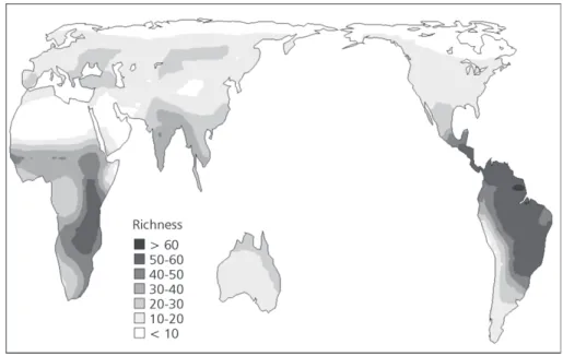
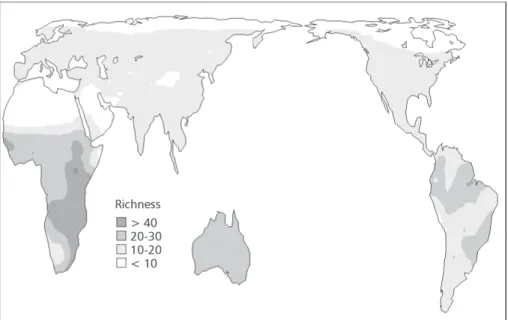
The species richness of Falconiformes around the world does not follow a simple latitudinal gradient in two dimensions, with complex variations within each continent, both for all species (Fig. 1) and species endemic to each domain (Fig. 2). In ge-neral, the higher diversities are at lower latitudes near the Equator; at higher latitudes, species richness tends to be lower.
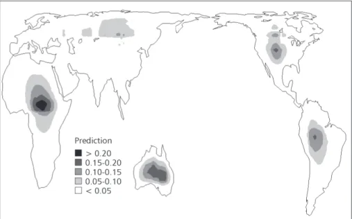
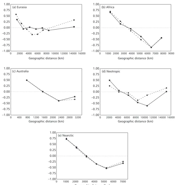
High diversities of all species of Falconiformes are in the northeastern Neotropics and in central-eastern sub-Saharan Africa, while the lower ones are in the higher latitudes of the northern hemisphere, and in Saharan Africa (Fig. 1). A high richness of endemic Falconiformes is also found in central-eastern sub-Saharan Africa (Fig. 2). Spatial patterns of species richness for all species and endemics are only slightly similar around the world (r2 = 0.5140), with highest similarities in Africa and Australia (r2 = 0.9254) and lowest in the Neotropics (r2 = 0.3136). Analyzing the predictions of the different null models used (Figs. 3 and 4), we can easily note their underlying differences. The WL2D always predicts high richness in the middle of domains, regardless of their range, and the estimated values decrease in a regular gradient toward the borders (Fig. 3). On the other hand, in the AC-WL2D there are only isolated peaks in the center of the domains (Fig. 4). The coefficients of determination of the linear regressions between observed and expected richness under the null models were always very low (Tables 1 and 2). However, the spatial correlograms usually indicated a significant autocorrelation for species richness in the different regions. There are usually strong positive autocorrelations at small spatial scales (first distance classes), followed by a monotonic decay of autocorrelation with distance, with a
reversal of the gradient in the last distance classes (Fig. 5).
When considering all species, coefficients of determination were usually low, and except for the whole world (WL2D: r2 = 0.0729; p = 0.0001 and AC-WL2D: r2 = 0.0605; p = 0.0114), none was significant at 5% level (Table 1). However, it is important to note that the degrees of freedom for the entire world were defined by summing the degrees of freedom for the different regions, since a world-scale autocorrelation analysis is meanin-gless. This while this number of degrees of freedom may still be overestimated, the most important fact is the very low r2 for both models (less than 10%) Using only endemic species, the coefficients are slight larger, and only coefficients for the whole world (WL2D: r2 = 0.1089; p = 0.0001 and AC-WL2D: r2 = 0.1030; p = 0.0027), Eurasia (WL2D: r2 = 0.1127; p = 0.0161), and Nearctic (WL2D: r2 = 0.1050; p = 0.0307) were significant at the 5% level (Table 2).
The NPP is usually higher at lower latitudes, in a conspicuous latitudinal gradient, with the maxi-mums close to the Equator, in tropical climates (see Brown & Lomolino, 1998). The highest production of biomass per surface area is in the Amazon, western and central sub-Saharan Africa, and south-western India, while the lowest values is in the
deserts, northern Africa, the center of Asia and Australia, and also in cold zones, such as northern North America and northern Asia. The NPP was a much better predictor of richness of Falconiformes around the world (r2 = 0.5027; p = 0.0001 for all species and r2 = 0.3352; p = 0.0001 for endemics only), with most coefficients being significant at the 5% level. The higher r2 were obtained in Australia, when analyzing all species (r2 = 0.5640; p = 0.0167),
and also with endemics only (r2 = 0.5595; p = 0.0160). The weakest and non-significant coefficients were for endemic species in the Neotropics (r2 = 0.1239; p = 0.1310) and in Eurasia (r2 = 0.1529; p = 0.0726) (Table 3). Since NPP is independent of the two MDE measures, partial correlations between richness and WL2D and WL2D-AC (keeping NPP constant) remain qualitatively unchanged.
WL2D null model AC-WL2D null model
Domain n spp n pts
r2 D. F. p r2 D. F. p
Worldwide 254 1430 0.0729 211.7 0.0001 0.0605 103.1 0.0114
Eurasia 82 576 0.0097 103.1 0.3160 0.0017 45.9 0.7775
Africa 91 340 0.0363 23.0 0.3607 0.0150 16.1 0.6260
Australia 25 88 0.1887 15.3 0.0785 0.1644 12.5 0.1420
Neotropic 91 227 0.0924 24.0 0.1314 0.0560 15.2 0.3573
Nearctic 39 199 0.0977 46.3 0.0510 0.1502 13.4 0.1466
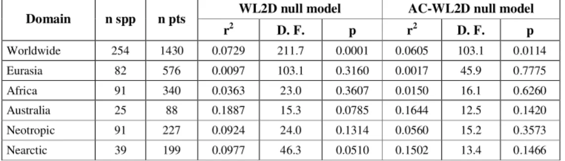
TABLE 1
Coefficients of determination (r2) of species richness regressed against predicted diversity by each null model, for all
species of Falconiformes worldwide and for each domain separately. The number of points in the grid is “n pts”, while the number of species in each domain is “n spp”. The degrees of freedom (D.F.) were given by taking into account the spatial autocorrelation in data, as suggested by Dutilleul (1993), giving a more appropriate estimate of
Type I error of regression coefficient (p).
WL2D null model AC-WL2D null model
Domain n spp n pts
r2 D. F. p r2 D. F. p
Worldwide 189 1430 0.1089 169.6 0.0001 0.1030 82.6 0.0027
Eurasia 41 576 0.1127 48.8 0.0161 0.0559 16.8 0.3311
Africa 56 340 0.0541 22.7 0.2707 0.0123 14.8 0.6731
Australia 19 88 0.1174 16.6 0.1556 0.1077 13.5 0.2215
Neotropic 65 227 0.0298 39.0 0.2799 0.0712 24.8 0.2163
Nearctic 8 199 0.1050 42.5 0.0307 0.2150 12.7 0.0849
TABLE 2
Coefficients of determination (r2) of species richness regressed against predicted diversity by each null model, for
worldwide endemic species of Falconiformes and for each domain separately. The number of points in the grid is “n
pts”, while the number of species in each domain is “n spp”. The degrees of freedom (D.F.) were given by taking into account the spatial autocorrelation in the data, as suggested by Dutilleul (1993), giving a more appropriate estimate
of Type I error of regression coefficient (p).
All species Endemic species
Domain n pts
n spp r2 D. F. p n spp r2 D. F. p
Worldwide 1430 254 0.5027 76.8 0.0001 189 0.3352 64.8 0.0001
Eurasia 576 82 0.4276 39.3 0.0001 41 0.1529 19.8 0.0726
Africa 340 91 0.4419 8.3 0.0315 56 0.5446 6.9 0.0238
Australia 88 25 0.5640 7.3 0.0167 19 0.5595 7.5 0.0160
Neotropic 227 91 0.5041 9.4 0.0122 65 0.1239 17.7 0.1310
Nearctic 199 39 0.4489 12.5 0.0073 8 0.3528 12.9 0.0199
TABLE 3
Coefficients of determination (r2), between the net primary productivity (NPP) against diversities of Falconiformes.
–1.00 –0.75 –0.50 –0.25 0.00 0.25 0.50 0.75 1.00
(a) Eurasia
–1.00 –0.75 –0.50 –0.25 0.00 0.25 0.50 0.75 1.00
(b) Africa
–1.00 –0.75 –0.50 –0.25 0.00 0.25 0.50 0.75 1.00
(c) Australia
–1.00 –0.75 –0.50 –0.25 0.00 0.25 0.50 0.75 1.00
0 2000 4000 6000 8000 10000 12000 14000 16000 0 1000 2000 3000 4000 5000 6000 7000 8000 9000
0 400 800 1200 1600 2000 2400 2800 3200 0 2000 4000 6000 8000 10000 12000 14000 16000 (d) Neotropic
–1.00 –0.75 –0.50 –0.25 0.00 0.25 0.50 0.75 1.00
0 1000 2000 3000 4000 5000 6000 7000 (e) Nearctic
Geographic distance (km) Geographic distance (km)
Geographic distance (km) Geographic distance (km)
Geographic distance (km)
Fig. 5 — Correlograms of species diversity of Falconiformes for (a) Eurasia, (b) Africa, (c) Australia, (d) Neotropic, and (e) Nearctic. The continuous line with squares is the Moran’s I estimated for the whole pool of species, while the dashed line with dots is for the endemic species only.
DISCUSSION
The species richness of Falconiformes is strongly spatially patterned over the world, although these patterns cannot be expressed as simple bi-dimensional gradients within domains. Since the correspondence between observed and expected richness under bi-dimensional null models is very weak, richness patterns cannot be interpreted only as a function of continental edges, as predicted by
the mid-domain effect. Therefore, richness is not simply caused by a random overlap of constrained geographical ranges, and, thus, other environmental factors should be invoked to explain it. This result is congruent with all other bi-dimensional analyses of the mid-domain effect (Bokma et al., 2001; Jetz & Rahbek, 2001; Diniz-Filho et al., 2002; Hawkins & Diniz-Filho, 2002).
distribution patterns, based on chance alone, which allows testing isolated biological mechanisms (Gotteli, 2001). Thus, to test the MDE using a null model is to ask whether a randomized pattern can reproduce one based on real data, and excluding from the test any other important features (i.e., environment and specific characteristics).
Probably the most improper assumption of the MDE is about the underlying factors entailed by the definition of range per se. As pointed out by Brown et al. (1996), range is a "complex of spatial and temporal patterns in which individual organisms are dispersed over the earth" and includes various features, such as size, shape, boundaries, and internal structure. Each of these features is influenced by many variables (such as ecologically limiting factors, environmental sustainability), which restrict the variation in distribution over a given space and, consequently, the richness of species.
Actually, each species has a unique ecological niche resulting from a complex of interactions between environmental variables that determine the distribution of the specie over the domain. Only within a specific set of parameter values, survival and reproduction can occur. The niche variables, independently or not of any other set of variables, determine a local range boundary, and limit local or regional distribution at different locations around the periphery (Brown et al., 1996). Hence, domains cannot be understood as homogeneous surfaces, without any internal boundaries or possible interac-tive features allowing species to easily spread over a space independently, and randomly across direc-tions. There are actually many boundaries (so-called soft boundaries), e.g., environmental and ecological ones (Hawkins & Diniz-Filho, 2002).
In sum, the complex interactions between abiotic and biotic features cannot be isolated from geographic ranges, as MDE does, since geographic occurrence is not the primary cause of observed richness, but rather the result of various interactions between species and environment. Therefore, MDE, due to all of its spanned assumptions, does not reasonably fit the final richness in observed data. Even a crude measure of an environmental factor (i.e., NPP), as used here, explains much more of variance of richness across bi-dimensional space than does the mid-domain null model. Also, MDE does not explain even the resi-dual variation in richness after taking into account the environment. Of course, a future step is to test
the response of the richness to NPP using better-quality data, at finer spatial scales.
Although the hypothesis that boundaries could constrain the spatial distribution of the ranges over a domain has recently reached generalized accep-tance, it is based on mistaken assumptions about the definition of ranges and domains (Hawkins & Diniz-Filho, 2002).
Acknowledgments — We thank Luis Mauricio Bini and Bradford A. Hawkins for previous discussions on the mid-domain effect. Our research program on biogeography, macroecology, biodiversity, and quantitative ecology has received supported from the Conselho Nacional de Desenvolvimento Científico e Tecnológico (CNPq, procs.: 101379/02-1 and 300762/94-1) and by FUNAPE/UFG.
REFERENCES
BINI, L. M., DINIZ-FILHO, J. A. F., BONFIM, F. S. & BASTOS, R. P., 2000, Local and regional species richness relationships in Viperid snake assemblages from South America: unsaturated patterns three different spatial scales. Copeia,
2000: 799-805.
BOKMA, F. & MÖNKKÖNEN, M., 2000, The mid-domain effect and the longitudinal dimension of continents. Trends Ecol. Evol., 15: 288-289.
BOKMA, F., BOKMA, J. & MÖNKKÖNEN, M., 2001, Random processes and geographic species richness patterns: why so few species in the north? Ecography, 24: 43-49.
BLACKBURN, T. M. & RUGGIERO, A., 2001, Latitude, elevation and body mass variation in Andean passerine birds.
Global Ecology & Biogeography, 10: 245-259. BROWN, J. H., STEVENS, G. C. & KAUFMAN, D. M., 1996,
The geographic range: size, shape, boundaries, and internal structure. Annu. Rev. Ecol. Syst., 27: 597-623.
BROWN, J. H. & LOMOLINO, M. V., 1998, Biogeography, 2nd Ed., Sinauer Associates, USA.
COLWELL, R. K. & LEES, D. C., 2000, The mid-domain effect: geometric constraints on the geography of species richness.
Trends Ecol. Evol., 15: 70-76.
COLWELL, R. K. & HURT, G. C., 1994, Nonbiological gradients in species richness and a spurious Rapoport effect. American Naturalist, 144: 570-595.
CURRIE, D. J., 1991, Energy and large-scale patterns of animal-and plant-species richness. American Naturalist, 137: 27-49. DEL HOYO, J., ELLIOT, A. & SARGATAL, J., 1994, Handbook of the birds of the world. Vol 2. New world vultures to Guineafowl, Lynx ediciones, Barcelona.
DINIZ-FILHO, J. A. F., DE SANT'ANA, C. E. R., DE SOUZA, M. C. & RANGEL, T. F. L. V. B., 2002, Null models and spatial patterns of species richness in South American birds of prey. Ecology Letters, 5: 47-55.
GOTTELI, N. J., 2001, Research frontiers in null model analysis.
Global Ecology & Biogeography, 10: 337-343. GUÉGAN, J-F., LEK, S. & OBERDORFF, T., 1998, Energy
availability and habitat heterogeneity predict global riverine fish diversity. Nature, 391: 382-384.
HAWKINS, B. A. & DINIZ-FILHO, J. A. F., 2002. The mid-domain effect and the species richness of Neartic birds.
Global Ecology & Biogeography, 11: In Press.
HAWKINS, B. A. & PORTER, E., 2001, Area and the latitudinal diversity gradient for terrestrial birds. Ecology Letters, 4:
595-601.
JETZ, W. & RAHBEK, C., 2001, Geometric constraints explain much of the species richness pattern in African birds. Proc. Natl. Acad. Sci., USA, 98: 5661-5666.
KOLEFF, P. & GASTON, K. J., 2001, Latitudinal gradients in diversity: real patterns and random models. Ecography, 24:
341-351.
LEGENDRE, P. & LEGENDRE, L., 1998, Numerical Ecology. 2nd English edn. Elsevier, Amsterdan.
LEGENDRE, P., 2000, T-test for a Pearson correlation coefficient corrected for spatial autocorrelation following Dutilleul (1993). R-Package. Freely downloadable at http://www.fas.
umontreal.ca/biol/casgrain/en/labo/mod_t_test.html. RAHBEK, C. & GRAVES, G. R., 2001, Multiscale assessment
of patterns of avian species richness. Proc. Natl. Acad. Sci.
USA, 98: 4534-4539.
RODHE, K., 1992, Latitudinal gradients in species diversity: the search for the primary cause. Oikos, 65: 514-527. ROSENZWEIG, M. L., 1995, Species diversity in space and
time. Cambridge University Press, Cambridge, USA.
RUGGIERO, A., 1999, Spatial patterns in the diversity of mammal species: A test of geographic area hypothesis in South America. Ecoscience, 6: 338-354.
SCHALL, J. J. & PIANKA, E. R., 1977, Species densities of reptiles and amphibians on the Iberian Peninsuls. Acta Vetebrata, 4: 27-34.
SCHALL, J. J. & PIANKA, E. R., 1978, Geographical trends in numbers of species. Science, 201: 679-686.
TURNER, J. R. G., GATEHOUSE, C. M. & COREY, C. A., 1987, Does solar energy control organic diversity? Butterflies, moths and the British climate. Oikos, 48: 195-205. TURNER, J. R. G., LENNON, J. J. & LAWRENSON, J. A.,
1988, British bird species distributions and the energy theory.
Nature, 335: 539-541.
VON HUMBOLDT, A., 1807, Ansichten der Natur mit wissenschaftlichen Erlauterungen. J. G. Cotta, Tübingen,
Germany.
WHITTAKER, R. J., WILLIS, K. J. & FIELD, R., 2001, Scale and species richness: towards a general, hierarchical theory of species diversity. Journal of Biogeography, 28: 453-470.
WILLIAMS, P. H., 2000, Worldmap iv Windows: Software version 4.20.05 (29.IV.2000). Public Demo, London.
WILLIG, M. R. & LYONS, S. K., 1998, An analytical model of latitudinal gradients of species richness with an empirical test for marsupials and bats in the New World. Oikos, 81:
93-98.