Digital quadrature demodulation of Doppler signals

(1)

UNIVERSIDADE DO ALGARVE

Faculdade de Ciˆencias e Tecnologia

Digital Quadrature Demodulation

of Doppler Signals

Manuel Mateus e Silva Rocha

Mestrado em Engenharia Electr´onica e Telecomunica¸c˜oes

especialidade de Processamento de Sinal

(2)

Faculdade de Ciˆencias e Tecnologia

Digital Quadrature Demodulation

of Doppler Signals

Manuel Mateus e Silva Rocha

Disserta¸c˜

ao orientada por:

Maria da Gra¸ca Cristo dos Santos Lopes Ruano

Mestrado em Engenharia Electr´onica e Telecomunica¸c˜oes

especialidade de Processamento de Sinal

(3)

Resumo

A descobertas dos ultrassons deu-se em 1880 [39]. A utiliza¸cão de ultrassons como ferramenta de diagnóstico existe há pelo menos 4 décadas [28]. O uso de ultrassons tem abrangido diversas áreas deste a deteçcão e quantifica¸cão de obstru¸cões no sistema cardiovascular [79], à deteçcão de gravidez e avalia¸cão de vários aspectos na saúde do feto, bem como à localiza¸cão e medi¸cão dos cálculos renais. A utiliza¸cão dos ultrassons no diagnóstico tem sofrido uma evolu¸cão crescente permitindo actualmente a identifica¸cão de micro-êmbolos bem como a sua caracteriza¸cão em termos da constitui¸cão e dimensão [79]. As técnicas de ultrassom têm igualmente evolu´ıdo de forma a possibilitar a apresenta¸cão dos resultados em imagens 2D coloridas [1], bem como imagens 3D [86] como as aplicadas para visualizar o feto num espa¸co tridimensional.

Se considerarmos o caso espec´ıfico do diagnóstico aplicado à deteçcão e quantifica¸cão ao n´ıvel do sistema cardiovascular os ultrassons podem ser aplicados de diferentes formas, permitindo a obten¸cão qualitativa e quantitativa de várias informa¸cões. Actualmente e inserido no projecto Desarrollo de Sistemas Ultrasónicos y Computacionales para Diagnóstico Cardiovascular (SUCoDiC) [85] a informa¸cão recolhida com recurso aos ultrassons é proveniente de três técnicas: Avalia¸cão do fluxo sangu´ıneo através do efeito de Doppler [40][41][42], medi¸cão do volume de fluxo sangu´ıneo através das técnicas de Transit-Time Flow Measurements (TTFM) [36] e o estudo das propriedades mecânicas das paredes dos vasos sangu´ıneos através da técnica de elastografia [37] [38].

No contexto do projecto mencionado, estas três técnicas são aplicadas para avaliar a qualidade de conjuntos de bypasses realizados durante cirurgias card´ıacas. Com recurso a estas técnicas o cirurgião determina, durante a cirurgia, se cada bypass criado conduz uma quantidade de fluxo sangu´ıneo adequada e, recorrendo à tecnica de elastografia avalia se as propriedades mecânicas da veia a utilizar no bypass por forma a evitar que futuramente o paciente tenha de sujeitar-se a nova opera¸cão. A combina¸cão das três técnicas durante a interven¸cão cirúrgica possibilitam a diminui¸cão de problemas pós-operatórios, na medida em que auxiliam os cirurgiões através de imagens e da quantifica¸cão de parâmetros cruciais no momento de avaliar a qualidade de cada bypass aplicado.

Convém igualmente referir que os ultrassons são uma ferramenta muito eficaz em diversas áreas, não estando estas limitadas à medicina. Podemos encontrar exemplos de aplica¸cões dos ultrassons noutras áreas como na indústria (para limpeza de materiais, processos qu´ımicos, desgaseifica¸cão de solventes, obten¸cão de informa¸cões sobre defeitos [39]) , em sistemas de localiza¸cão em interiores (indoor location) (reportando-se serem mais precisos do que sistemas baseados em infravermelhos,

(4)

radio-frequência ou sensores no chão [84]), entre outras áreas.

O trabalho realizado nesta tese enquadra-se no processamento de sinais biomédicos obtidos por ultrassom de Doppler. No projecto SUCoDiC, um sistema analógico [40] é responsável pelo proces-samento dos sinais de ultrassom resultantes do retro-espalhamento das part´ıculas contidas no fluxo sangu´ıneo. Neste sistema, os sinais de ultrassons recebidos são desmodulados analogicamente por forma a obterem-se as componentes em fase (I) e em quadratura (Q) do respectivo sinal. Estas duas componentes são posteriormente utilizadas para a obten¸cão de informa¸cão sobre a direçcão do fluxo sangu´ıneo através do seu processamento digital. Foi, no entanto, verificado que a existência de um desiquil´ıbrio nos ganhos nos canais do desmodulador (um canal para a componente em fase e outro para a componente em quadratura) provoca problemas na separa¸cão do fluxo directo e reverso.

Através das pesquisas realizadas, verificou-se que os desmoduladores digitais em quadratura são sugeridos como alternativas ao desmodulador analógico actualmente utilizado no referido projecto. De facto, o recurso aos desmoduladores em fase e em quadratura digitais permite solucionar problemas associados a ganhos desiguais, diferen¸cas de fase diferentes de 90o _{e ainda varia¸cões do valor das}

componentes DC entre os canais relativos `as componentes em fase e em quadratura.

O resurso a técnicas digitais para realizar o processamento dos sinais e consequente obten¸cão das componentes em fase e em quadratura, apresenta igualmente vantagens associadas à flexibilidade destas técnicas, no que respeita à altera¸cão de parâmetros de uma determinada técnica, bem como à flexibilidade de substitui¸cão de uma técnica por outra. Associado a esta flexibilidade surge igualmente a rapidez com que as altera¸cões podem ser feitas.

Devido às caracter´ısticas inerentes ao ultrassom utilizado foram encontradas, na prática, limita¸cões impostas pelo conversor analógico-para-digital em rela¸cão à frequência de amostragem poss´ıvel de ser utilizada. Como forma de contornar este obstáculo duas estratégias foram implementadas. Numa, recorrendo à fun¸cão heteródina, os sinais de ultrassons, no dom´ınio da rádio-frequência, são deslo-cados para portadoras de frequência inferior, permitindo desta forma a amostragem dos sinais sem que ocorra aliase. Outra estratégia, recorre a uma amostragem passabanda uniforme, e realiza a amostragem directa dos sinais de ultrassons no dom´ınio da rádio-frequência, onde a frequência de amostragem é seleccionada por forma a criar uma aliase deliberada nos sinais de rádio-frequência. Ao criarem-se aliases do sinal desejado faz-se a sua transla¸cão espectral para uma frequência conhecida sem, no entanto, causar aliase no conteúdo do sinal.

A pesquisa realizada sobre técnicas digitais de quadratura foi concentrada no estudo de cinco abordagens digitais para a obten¸cão das componentes em fase e em quadratura. Três técnicas digitais de quadratura são sugeridas como alternativas viáveis ao desmodulador analógico e consequentemente deverão ser implementadas e testadas em processamento em tempo real.

Associado ao trabalho de processamento digital de sinal, foram igualmente desenvolvidas nesta tese aplica¸cões em software e firmware com vista ao controlo de dispositivos, quer comerciais, quer desenvolvidos no decorrer deste trabalho. Para além da componente de software, vários módulos de hardware foram criados, como sendo, um circuito controlador de uma bomba de fluxo, um módulo

(5)

iii regulador de tensão, um módulo contendo um sintetizador de frequências baseado numa Phase Locked

Loop (PLL) e ainda um m´odulo contendo um multiplicador anal´ogico, filtros e um amplificador

sintonizado.

A avalia¸cão das técnicas digitais de quadratura é realizada recorrendo a um sinal de teste, simula-do, que permitiu uma boa caracteriza¸cão de inúmeros aspectos relativos à performance de cada uma das técnicas. No campo experimental, sinais cujo conteúdo espectral é conhecido e bem caracterizado foram produzidos por geradores de fun¸cões e, amostrados recorrendo às duas estratégias referidas (utiliza¸cão da fun¸cão heteródina e amostragem passabanda uniforme).

Os resultados obtidos pelas diferentes metodologias propostas são apresentados, criticados e, apontam-se as solu¸cões que se consideram mais relevantes para integra¸cão no projecto de investiga¸cão no qual este trabalho se insere.

Palavras-Chave: Amostragem Passabanda, Doppler, Fluxo Sangu´ıneo, Quadratura Digital, Fun¸c˜ao Heter´odina

(6)

Ultrasound has for many years been an important tool in the detection and quantification of various health problems. In vascular diseases, for example, the ultrasound can be applied with different techniques such as Transit-Time Flow Measurements (TTFM) [36], Doppler [28][40][41][42] and elas-tography [37] [38].

Research has been developed focusing the signal processing of Doppler ultrasound signals. In an ongoing project, named Desarrollo de Sistemas Ultras´onicos y Computacionales para Diagn´ostico Cardiovascular (SUCoDiC), Doppler ultrasound signals are processed by an analog signal processing unit, in order to obtain the inphase (I) and quadrature (Q) components of the Doppler ultrasound signals, to allow directional blood flow separation.

Problems associated with unbalanced channels’ gain of the employed analog system have been detected, resulting in an inapropriate directional blood flow separation.

This thesis reports the research performed to eliminate such problems by substituting the analog system’s demodulator by digital signal processing approaches aiming at the achievement of the same goals, i.e., obtaining the Doppler ultrasound signal’s inphase (I) and quadrature (Q) components, for efficient directional blood flow separation.

Five digital quadrature techniques have been studied to achieve such goal. Also, given technical constraints imposed by the nature of the Doppler ultrasound signals to be used, and limitations of the sampling rate of the Analog-to-Digital Converter (ADC) used, two strategies to acquire the Doppler ultrasound signals were studied. Such strategies involved the sampling of a downconversion version of the Doppler ultrasound signals (by application of the heterodyne function) and direct sampling of the Doppler ultrasound signals using uniform bandpass sampling.

From the results obtained, three approaches are selected and proposed for real time implementa-tion. Comparison between both signal sampling strategies employed are also presented.

Keywords: Bandpass Sampling, Doppler, Blood Flow, Digital Quadrature, Heterodyne Func-tion

(7)

Agradecimentos

Primeiramente quero agradecer à minha orientadora Professora Doutora Maria da Gra¸ca Cristo dos Santos Lopes Ruano, pelo convite inicial, pelo apoio e amizade ao longo deste mestrado e pelas condi¸cões de trabalho proporcionadas para que nada faltasse em termos materiais. Gra¸cas aos seus conselhos e orienta¸cão foi poss´ıvel, nos momentos dif´ıceis, reflectir e encontrar caminhos para seguir sempre em frente.

Quero igualmente agradecer aos restantes membros do Grupo de Processamento de Sinal Biomédico, nomeadamente à Professora Doutora Maria Margarida Madeira e Moura e à Professora Doutora Ana Isabel Leiria pelas sugestões apresentadas por elas no in´ıcio do trabalho, ao Engenheiro Sérgio Silva pela sua ajuda nalgumas aplica¸cões criadas em linguagem Python, e um agradecimento especial ao Doutor César Teixeira pelas suas sugestões e pela troca de ideias ao longo de todo o trabalho realizado.

Quero agradecer `a Let´ıcia Costa, minha namorada, pelo carinho, pela imensa paciˆencia e pelo apoio demonstrado ao longo deste mestrado.

Um agradecimento muito especial aos meus pais que sempre me apoiaram, ajudaram e pela muita paciˆencia que tˆem tido.

Por fim quero fazer um agradecimento aos meus amigos e colegas de curso que me ajudaram durante o curso, em especial ao Eduardo Domingues Gon¸calves, grande amigo e colega de curso, que ao longo de v´arios anos neste curso, sempre apresentou o seu apoio e ajuda.

(8)

1 Introduction 1

1.1 Motivation . . . 1

1.2 Proposed goals . . . 3

1.3 Thesis outline . . . 3

2 General Concepts on Doppler Ultrasound Systems 6 2.1 Introduction . . . 6

2.2 Doppler Shift . . . 6

2.3 Ultrasound backscattered from blood . . . 7

2.4 Basic Doppler Systems . . . 9

2.4.1 The Demodulator . . . 11

3 Doppler Ultrasound System’s Demodulators 13 3.1 Heterodyning Function . . . 13

3.1.1 Introduction . . . 13

3.1.2 Phase Locked Loop . . . 16

3.2 Bandpass Sampling . . . 21

3.2.2 Bandpass Sampling (BPS) Frequency Selection . . . 23

3.2.3 Uniform Sampling . . . 23

3.2.4 Spectral Inversion . . . 26

3.2.5 BPS Disadvantages . . . 26

3.3 Digital Quadrature Techniques . . . 27

3.3.2 Bandpass Signal Representation . . . 28

3.3.3 Complex Sampling . . . 29

4 Experimental Setup Developed 38 4.1 Introduction . . . 38

4.2 Experimental Setup Implemented . . . 39

4.2.1 Equipment used . . . 39 vi

(9)

CONTENTS vii

4.2.2 Flow Pump Control . . . 40

4.2.3 Signal Acquisition . . . 42

4.2.4 NI DAQ USB 6251 Control Software Application . . . 47

4.3 Digital Techniques Parametrization . . . 49

4.3.1 Testing and Experimental Signal’s Characterization . . . 49

4.3.2 BPS Frequency Determination . . . 53

4.3.3 Separation between Forward and Reverse Flow . . . 54

4.3.4 Filters to be Used . . . 55

5 Results Obtained with the 5 Approaches Implemented 59 5.1 Results of the Different Demodulator Circuitry Approaches Using the Developed Testing Signals . . . 59

5.1.2 Approach 1: signal without noise . . . 60

5.1.3 Approach 1: signal with noise . . . 62

5.1.12 Bandpass Sampling . . . 78

5.1.13 Comments on the Testing Signal Results . . . 79

5.2 Results of Bandpass Sampling when Experimental Signals are Used . . . 81

5.2.1 Introduction . . . 81 5.2.2 Approach 1 . . . 84 5.2.3 Approach 2 . . . 85 5.2.4 Approach 3 . . . 86 5.2.5 Approach 4 . . . 87 5.2.6 Approach 5 . . . 88

5.2.7 Comments on the Experimental Signal Results Obtained by BPS Technique . 89 5.3 Results Obtained after Heterodyne Application on Experimental Signals . . . 90

5.3.2 Approach 1 . . . 92

(10)

5.3.4 Approach 3 . . . 94

5.3.5 Approach 4 . . . 95

5.3.6 Approach 5 . . . 96

5.3.7 Comments on the Experimental Signal Results Obtained After Heterodyne Technique . . . 97

6 Discussion of the Results and Concluding Remarks 98 6.1 Introduction . . . 98

6.2 Generic Considerations . . . 99

6.3 General Conclusions . . . 101

6.4 Future research lines . . . 102

7 Appendixes 103 A Acronyms 104 B Relationship between allowed sampling frequencies in [6] and [50] 106 C PLL-based Frequency Syntesizer Characterization Plots 109 C.1 Results for ξ=0.65 . . . 110

C.2 Results for ξ=0.707 . . . 113

C.3 Results for ξ=0.80 . . . 116

C.4 Results for ξ=0.90 . . . 119

D Predicted Spectra for signals I′′_{(t) and Q}′′_(t) ₁₂₂ E I′′_{(n) and Q}′′_{(n) Magnitude Spectra Behaviour} ₁₂₈ F Characteristics of the Filters Employed 131 F.1 Lowpass Filters Used in Approach 1 . . . 132

F.1.1 For Results Using the Testing Signals . . . 132

F.1.2 For Results of BPS when Experimental Signals are used . . . 135

F.1.3 For Results after Heterodyne Function Application on Experimental Signals . 135 F.2 Lowpass Filters Used in Approaches 2 to 4 . . . 136

F.2.2 For Results of BPS when Experimental Signals are used . . . 139

F.2.3 For Results after Heterodyne Function Application on Experimental Signals . 140 F.3 Lowpass Filters Used in Approach 5 . . . 141

F.3.2 For Results of BPS when Experimental Signals are used . . . 150 F.3.3 For Results after Heterodyne Function Application on Experimental Signals . 151

(11)

CONTENTS ix F.4 Allpass Filters Used in Approach4 . . . 153

G PCB and Perfboard Images 158

(12)

2.1 Block diagram of a continuous wave Doppler system (Adapted from figure 6.1 in [28] and from figure 1 in [45] . . . 9 2.2 Block diagram of a pulsed wave Doppler system (Adapted from figure 6.11 in [28]) . . 10 2.3 Block diagram of a Single Sideband Detection (SSB) demodulator (Adapted from

figure 6.6 in [28]), where ωc stands for the filter cutoff frequency, ω0 stands for the

carrier frequency of the radiofrequency (RF) signal, and ωF and ωR are, respectively,

the frequencies associated with the forward and reverse flow . . . 11 2.4 Block diagram of a heterodyne demodulator (Adapted from figure 6.7 in [28]), where

ωH stands for the heterodyne frequency and ω0 stands for the carrier frequency of the

RF signal. . . 12 2.5 Block diagram of a quadrature phase detection demodulator(figure 6.8 in [28]), where

ω0 stands for the carrier frequency of the RF signal . . . 12

3.1 Block diagram of a continuous wave Doppler system, where the RF signal contain-ing the Doppler frequency shift information is downconverted to an Intermediate Frequency (IF) signal and sampled . . . 14 3.2 Block diagram of a pulsed wave Doppler system, where the RF signal containing the

Doppler frequency shift information is downconverted to an IF signal and sampled . . 14 3.3 Block diagram of the heterodyne technique used to obtain the IF signal. The local

oscillator is a frequency synthesizer block, implemented using a PLL, where ω0 stands

for the master oscillator frequency (which is also the carrier frequency of the ultrasound wave) and ωLO stands for the local oscillator frequency. The frequency ωc = 2πfIF is

the value of the carrier frequency that the IF signal will have . . . 15 3.4 Spectral representation of the signals indicated in figure 3.3, where ω0, ωLO and ωc

have the same meaning as the ones presented in figure 3.3 . . . 16

(13)

LIST OF FIGURES xi 3.5 Mathematical model of a PLL in the locked state [17], where kd stands for the phase

comparator conversion gain, ko stands for the Voltage Controlled Oscillator (VCO)

conversion gain, F (s) is the loop filter transfer function, kn = _N1 with N being the

value by which the VCO output frequency is divided, θo and θi are, respectively, the

phase of the input (reference) signal of the PLL and the phase of the output signal (generated by the VCO) and θe if the phase error . . . 16

3.6 PLL locked state mathematical model with the Phase Detector (PD) block expanded [22], where kd stands for the phase comparator conversion gain, ko stands for the

Voltage Controlled Oscillator (VCO) conversion gain, F (s) is the loop filter transfer function, kn= _N1 is the feedback loop divider ratio, with N being the value by which

the VCO output frequency is divided, θo and θi are, respectively, the phase of the

input (reference) signal of the PLL and the phase of the output signal (generated by the VCO) and θe if the phase error . . . 17

3.7 Typical passive filter used in a PLL [17], where vi stands for the input signal and vo

stands for the output signal of the filter . . . 17 3.8 Block diagram of a continuous wave Doppler system, where the RF signal

contain-ing the Doppler frequency shift information is sampled by and ADC with a proper sampling rate . . . 22 3.9 Block diagram of a pulsed wave Doppler system, where the RF signal containing the

Doppler frequency shift information is sampled by and ADC with a proper sampling rate . . . 22 3.10 Spectrum of a bandpass continuous signal centered at a frequency f0 and total

band-width of B. The sampling frequency value is denoted by fs. Only positive frequencies

are presented (obtained from figure 1 in [50]) . . . 23 3.11 Spectrum of a bandpass continuous signal centered at a frequency f0and bandwidth of

B. To prevent aliasing an upper guard-band (BGU) and a lower guard-band (BGL) are

considered. The sampling frequency value is denoted by fs. Only positive frequencies

are presented (obtained from figure 5 in [50]) . . . 24 3.12 The allowed (white areas) and disallowed (shaded areas) for uniform sampling

fre-quencies versus band position. BGT = fs− 2B represents the total guard-band, fs the

sampling frequency and B is the bandwidth. (obtained from figure 4 in [50]) . . . 25 3.13 Typical complex sampling strategy using two analog channels and two ADC (Adapted

from [63]), where ω0 stands for the carrier frequency of the RF signal . . . 27

3.14 Magnitude spectrum of the IF signal sIF(t). SIF(jω) has a total bandwidth B,

cen-tered at a known carrier frequency ωc. . . 30

3.15 Magnitude spectrum of the digitized IF signal sIF(n), SIF(ejωT), where ωs stands for

(14)

3.16 Digital quadrature phase selection strategy used in approach 1, where ωs stands for

the used sampling frequency, ωc stands for the center frequency of the signal and B is

the signal’s total bandwidth. . . 31 3.17 Digital quadrature phase selection strategy used in approach 2 (Adapted from [6]),

where ωsstands for the used sampling frequency and ωc stands for the center frequency

of the signal. . . 32 3.18 Digital quadrature phase selection strategy used in approach 3 (Adapted from [8]),

of the signal. . . 36 4.1 Block diagram of the experimental apparatus main blocks . . . 38 4.2 Block diagram of path A shown in figure 4.1, where ωs stands for the sampling

fre-quency and B the total bandwith of the signal. In this path the BPS principles are used. . . 39 4.3 Block diagram of path B shown in figure 4.1, where ω1 stands for the local oscillator

frequency, ω0is the RF signal carrier frequency and ωcis the IF signal carrier frequency.

In this path the RF signal is down converted after applying the heterodyne technique. 39 4.4 Schematic diagram of the circuit built to control the flow pump motion through the

computer’s parallel port . . . 40 4.5 Graphical User Interface (GUI) interface for user input of the desired duty cycle and

period of the pulses to be generated. . . 41 4.6 Parallel port pins and associated memory registers [89] . . . 42 4.7 Tuned amplifier with central frequency of 8 MHz and an expected bandwidth of BW =

1

2π(10 kΩ)(390 pF ) = 40.8 kHz [93]. The practical −3 dB bandwidth ranges from 6.6 MHz

to 8.9 MHz. The capacitor in the BC337-16 transistor’s collector was later added (not soldered on the perfboard) to remove the signal’s DC component . . . 43 4.8 Schematic circuit of the PLL based frequency sinthesizer . . . 44 4.9 Block diagram of the PLL-based frequency synthesizer, indicating the values on each

frequency divider, the PLL reference oscillator and the output frequency synthesized by the circuit . . . 44 4.10 Schematic circuit of the RF signal mixer with the signal output (V COOU T) of the

(15)

LIST OF FIGURES xiii 4.11 Sallen-Key 6th order Lowpass Linear Phase with Equiripple Error of 0.05o _{filter, used}

to filter the output of the mixer (in figure 4.10) . . . 45 4.12 Passive filter used in a PLL [17], where vi stands for the input signal and vo stands

for the output signal of the filter . . . 46 4.13 GUI of the software used to setup the acquisition conditions of the NI DAQ USB 6251

device . . . 48 4.14 Magnitude spectrum of signal used to test the various strategies presented in

subsec-tion 3.3.3. The bottom figure is a zoom of the top figure, showing only frequency components from 45 kHz to 55 kHz. . . 53 4.15 Expected carrier and sideband components distribution for a sinusoidal carrier

mod-ulated by a sinusoidal signal, with β = 2 [14]. In the figure fc is the carrier frequency 53

4.16 Quadrature to Directional format using digital approaches {1, 3, 4} (Adapted from [48]), where F F (n) denotes forward flow signal and Rev F (n) denotes reverse flow signal . . . 55 4.17 Quadrature to Directional format using digital approaches {2, 5} (Adapted from [48]),

where F F (n) denotes forward flow signal and Rev F (n) denotes reverse flow signal . 55 4.18 Infinite Impulse Response (IIR) allpass notch filter used, defined by (4.3) with α = 0.995 56 4.19 Comb Finite Impulse Response (FIR) filter used for comparison with the allpass IIR

filter . . . 56 4.20 Magnitude spectra of an original signal with DC component and the filtered version

by the IIR allpass notch filter . . . 57 4.21 Magnitude spectra of an original signal with DC component and the filtered version

by the Comb FIR filter . . . 57 5.1 Magnitude spectra of the quadrature signals I”(n) and Q”(n) obtained when the

IF signal is multiplied by a cosine and a sine wave with frequency equal to the IF signal’s carrier frequency. The bottom figure is a zoom of the top figure, showing only frequency components from DC to 55 kHz. . . 60 5.2 Magnitude spectra of the quadrature signals I′_{(n) and Q}′_{(n), which result on the}

filtering of the signals whose spectrum is presented in figure 5.1 by the lowpass FIR filter in figure F.1. The bottom figure is a zoom of the top figure, showing only frequency components from DC to 45 kHz. . . 60 5.3 After the application of the DC notch filter of figure 4.18, the DC component is

attenuated. The bottom figure is a zoom of the top figure, showing only frequency components from -15 kHz to 15 kHz. . . 60 5.4 Comparison between the obtained and expected magnitude spectra for the forward

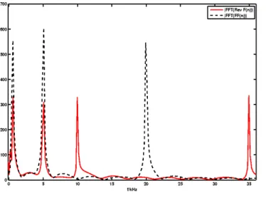
(top figure) and reverse (bottom figure) flow signals. As desired the 45 kHz component has been removed by the filtering. . . 60 5.5 Comparison between the obtained forward and reverse flow signals magnitude spectra. 61

(16)

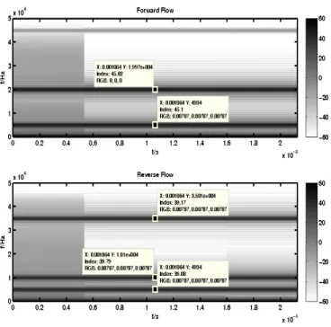
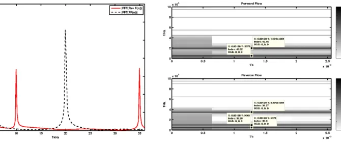
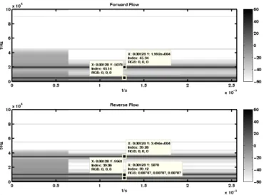
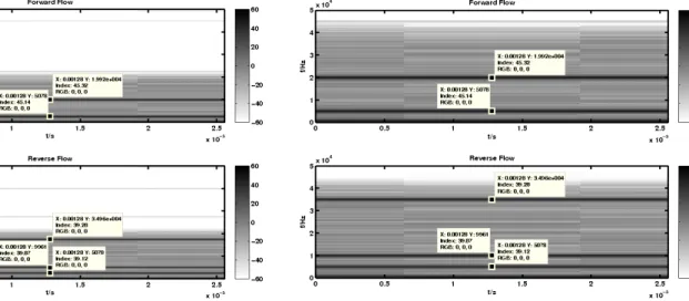
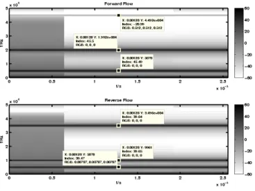
5.6 Spectrogram of the obtained forward and reverse flow signals . . . 61 5.7 Zoom of figure 5.6 on the important frequency range . . . 61 5.8 Spectrogram of the obtained forward and reverse flow signals, if the lowpass FIR filter

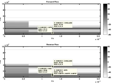
used has 80 dB stopband attenuation (figure F.2) . . . 62 5.9 Spectrogram of the obtained forward and reverse flow signals, if the lowpass FIR filter

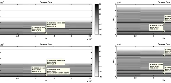
used has 120 dB stopband attenuation (figure F.3) . . . 62 5.10 Comparison between expected (without noise) and the obtained (with noise)

mag-nitude spectra for the forward (top figure) and reverse (bottom figure) flow sig-nals.(Lowpass FIR filter of figure F.2 was used). . . 62 5.11 Comparison between the obtained forward F F (n) and reverse Rev F (n) flow signals

magnitude . . . 62 5.12 Spectrogram of the obtained forward and reverse flow signals . . . 63 5.13 Zoom of figure 5.12 on the important frequency range . . . 63 5.14 Magnitude spectra of the quadrature signals I”(n) and Q”(n) obtained when the IF

signal is multiplied, respectively, by sequences +1, 0, −1, 0 and 0, 1, 0, −1 [6]. The bottom figure is a zoom of the top figure, showing only frequency components from DC to 50 kHz. . . 63 5.15 Magnitude spectra of the quadrature signals I′_{(n) and Q}′_{(n), which result on the}

filtering of the signals whose spectra are presented in figure 5.14 by the lowpass FIR filter in figure F.5. The bottom figure is a zoom of the top figure, showing only frequency components from DC to 45 kHz. . . 63 5.16 After the application of the DC notch filter of figure 4.18, the DC component is

(top figure) and reverse (bottom figure) flow signals. As desired the 45 kHz component has been removed by the filtering. . . 64 5.18 Comparison between the obtained forward F F (n) and reverse Rev F (n) flow signals

magnitude spectra. . . 64 5.19 Spectrogram of the obtained forward and reverse flow signals. . . 64 5.20 Zoom of figure 5.19 on the important frequency range . . . 65 5.21 Spectrogram of the obtained forward and reverse flow signals, if the lowpass FIR filter

used has 120 dB stopband attenuation (figure F.7) . . . 65 5.23 Comparison between expected (without noise) and the obtained ( with noise)

mag-nitude spectra for the forward (top figure) and reverse (bottom figure) flow signals. (Lowpass FIR filter of figure F.6 was used). . . 66

(17)

LIST OF FIGURES xv 5.24 Comparison between the obtained forward F F (n) and reverse Rev F (n) flow signals

magnitude spectra. . . 66 5.25 Spectrogram of the obtained forward and reverse flow signals . . . 66 5.26 Zoom of figure 5.25 on the important frequency range . . . 66 5.27 Magnitude spectra of the quadrature signals I”(n) and Q”(n). Q”(n) is obtained by

applying the Hilbert Transform to the IF signal.The bottom figure is a zoom of the top figure, showing only frequency components from DC to 50 kHz. . . 67 5.28 Magnitude spectra of the quadrature signals I′_{(n) and Q}′_{(n), which result on the}

magnitude spectra. . . 68 5.32 Spectrogram of the obtained forward and reverse flow signals . . . 68 5.33 Zoom of figure 5.32 on the important frequency range . . . 68 5.34 Spectrogram of the obtained forward and reverse flow signals, if the lowpass FIR filter

used has 120 dB stopband attenuation (figure F.7) . . . 69 5.36 Comparison between expected (without noise) and the obtained (with noise)

mag-nitude spectra for the forward (top figure) and reverse (bottom figure) flow signals. (Lowpass FIR filter of figure F.6 was used). . . 69 5.37 Comparison between the obtained forward F F (n) and reverse Rev F (n) flow signals

magnitude spectra. . . 69 5.38 Spectrogram of the obtained forward and reverse flow signals . . . 70 5.39 Zoom of figure 5.38 on the important frequency range . . . 70 5.40 Magnitude spectra of the quadrature signals I”(n) and Q”(n). These are obtained

by applying the 30th order allpass filters (figures F.39 and F.41, respectively). The bottom figure is a zoom of the top figure, showing only frequency components from DC to 50 kHz. . . 70

(18)

5.41 Magnitude spectra of the quadrature signals I′_{(n) and Q}′_{(n), which result on the}

(top figure) and reverse (bottom figure) flow signals (when used the 30th order allpass filters (figures F.39 and F.41). As desired the 45 kHz component has been removed by the filtering. . . 71 5.44 Comparison between the obtained forward F F (n) and reverse Rev F (n) flow signals

magnitude spectra (when used the 30th order allpass filters (figures F.39 and F.41). . 71 5.45 Spectrogram of the obtained forward and reverse flow signals (when used the 30th

order allpass filters (figures F.39 and F.41) . . . 71 5.46 Zoom of figure 5.45 on the important frequency range . . . 72 5.47 Spectrogram of the obtained forward and reverse flow signals, if the lowpass FIR filter

used has 81 dB stopband attenuation (figure F.6), when used the 30th order allpass filters (figures F.39 and F.41) . . . 72 5.48 Spectrogram of the obtained forward and reverse flow signals, if the lowpass FIR filter

used has 120 dB stopband attenuation (figure F.7), when used the 30th order allpass filters (figures F.39 and F.41) . . . 72 5.49 Comparison between the obtained forward F F (n) and reverse Rev F (n) flow signals

magnitude spectra, if the lowpass FIR filter used has 81 dB stopband attenuation (figure F.6) and 5th order allpass IIR filters are used (figures F.31 and F.33) . . . 73 5.50 Spectrogram of the obtained forward and reverse flow signals, if the lowpass FIR filter

used has 81 dB stopband attenuation (figure F.6) and 5th order allpass IIR filters are used (figures F.31 and F.33) . . . 73 5.51 Comparison between the obtained forward F F (n) and reverse Rev F (n) flow signals

magnitude spectra, if the lowpass FIR filter used has 81 dB stopband attenuation (figure F.6) and 15th order allpass IIR filters are used (figures F.35 and F.37) . . . 73 5.52 Spectrogram of the obtained forward and reverse flow signals, if the lowpass FIR filter

used has 81 dB stopband attenuation (figure F.6) and 15th order allpass IIR filters are used (figures F.35 and F.37) . . . 73 5.53 Comparison between expected (without noise) and the obtained (with noise)

mag-nitude spectra for the forward (top figure) and reverse (bottom figure) flow sig-nals.(Lowpass FIR filter of figure F.6 was used). . . 74

(19)

LIST OF FIGURES xvii 5.54 Comparison between the obtained forward F F (n) and reverse Rev F (n) flow signals

magnitude . . . 74 5.55 Spectrogram of the obtained forward and reverse flow signals . . . 74 5.56 Zoom of figure 5.55 on the important frequency range . . . 74 5.57 Magnitude spectra of the A(n) and B(n) signals. The bottom figure is a zoom of the

top figure, showing only frequency components from DC to 45 kHz. . . 75 5.58 Magnitude spectra of the I′_{(n) and Q}′_{(n) signals, obtained after application of filters}

in figures F.11 and F.12 respectively. The bottom figure is a zoom of the top figure, showing only frequency components from DC to 45 kHz. . . 75 5.59 After the application of the DC notch filter of figure 4.18, the DC component is

magnitude spectra, when filters in figures F.11 and F.12 are used. . . 76 5.62 Spectrogram of the obtained forward and reverse flow signals , when filters in figures

F.11 and F.12 are used . . . 76 5.63 Spectrogram of the obtained forward and reverse flow signals, when filters in figures

F.23 and F.24 are used . . . 77 5.67 Comparison between expected (without noise) and the obtained (with noise)

mag-nitude spectra for the forward (top figure) and reverse (bottom figure) flow signals. (filters in figures F.14 and F.15 are used). . . 77 5.68 Comparison between the obtained forward F F (n) and reverse Rev F (n) flow signals

magnitude . . . 77 5.69 Spectrogram of the obtained forward and reverse flow signals . . . 78 5.70 RF signal centered at a 8 MHz frequency carrier (see subsection 4.3.1). The bottom

figure is a zoom of the top figure, showing only frequency components from 7900 kHz to 8100 kHz. . . 78

(20)

5.71 Sampled signal using the allowed 240.604 kHz sampling rate. The signal is shifted to the expected frequency of 60.1 kHz (see subsection 4.3.2). The bottom figure is a zoom of the top figure, showing only frequency components from 50 kHz to 70 kHz. . 78 5.72 Spectrum of the FM signal, created by modulating a 8 MHz carrier with a 13 kHz sine

wave, with β = 2. The FM signal was sampled with a sampling rate of 240.604 kHz. The bottom figure is a zoom of the top figure, showing only frequency components from DC to 120 kHz. . . 81 5.73 Magnitude spectrum of signals I”(n) and Q”(n) in approach 2, when the sampling

frequency is not equal to four times the signal’s carrier frequency. It can be seen that the alignment of the spectra is not obtained. The bottom figure is a zoom of the top figure, showing only frequency components from DC to 50 kHz. . . 82 5.74 Magnitude spectrum of the acquired signal using BPS allowed frequency subjected

to resampling so that the new sampling frequency is equal to four times the signal’s carrier frequency. . . 83 5.75 Magnitude spectra of the obtained I(n) and Q(n) signals. The bottom figure is a

zoom of the top figure, showing only frequency components from DC to 40 kHz. . . . 84 5.76 Magnitude spectra of the obtained F F (n) and Rev F (n) signals. . . 84 5.77 Spectrogram of the obtained F F (n) and Rev F (n) signals. . . 84 5.78 Magnitude spectra of the obtained I(n) and Q(n) signals. The bottom figure is a

zoom of the top figure, showing only frequency components from DC to 40 kHz. . . . 88 5.88 Magnitude spectra of the obtained F F (n) and Rev F (n) signals. . . 88 5.89 Spectrogram of the obtained F F (n) and Rev F (n) signals. . . 88 5.90 Magnitude spectrum of the signal centered at 50 kHz, sampled at a frequency of 260

kHz . . . 91 5.91 Magnitude spectrum of the signal centered at 52.2 kHz, sampled at a frequency of

(21)

LIST OF FIGURES xix 5.92 Magnitude spectra of the obtained I(n) and Q(n) signals. The bottom figure is a

zoom of the top figure, showing only frequency components from DC to 40 kHz. . . . 94 5.99 Magnitude spectra of the obtained F F (n) and Rev F (n) signals. . . 94 5.100Spectrogram of the obtained F F (n) and Rev F (n) signals. . . 94 5.101Magnitude spectra of the obtained I(n) and Q(n) signals. The bottom figure is a

zoom of the top figure, showing only frequency components from DC to 40 kHz. . . . 95 5.102Magnitude spectra of the obtained F F (n) and Rev F (n) signals. . . 95 5.103Spectrogram of the obtained F F (n) and Rev F (n) signals. . . 95 5.104Magnitude spectra of the obtained I(n) and Q(n) signals. The bottom figure is a

zoom of the top figure, showing only frequency components from DC to 40 kHz. . . . 96 5.105Magnitude spectra of the obtained F F (n) and Rev F (n) signals. . . 96 5.106Spectrogram of the obtained F F (n) and Rev F (n) signals. . . 96 6.1 Figure presenting the block diagrams of all the five digital quadrature techniques on

section 3.3.3 . . . 99 6.2 Approaches to be considered for real-time implementation, as digital alternatives to

the currently used analog system’s demodulator in the SUCoDiC project . . . 102 B.1 Spectral replications of the bandpass continuous signal whose spectrum is presented

in (a), as the sampling frequency changes: (b) fs = 35MHz; (c) fs = 22.5MHz; (d)

fs = 17.5MHz; (e) fs = 15MHz; (f) fs = 11.25MHz;(g) fs = 7.5MHz;(Adapted

from figure 2-9 in [6]) . . . 108 C.1 Bode plot of the loop filter transfer function when ξ=0.65 and ωn= 615.38 rad/s . . 110

C.2 Bode plot of the feedforward transfer function when ξ=0.65 and ωn = 615.38 rad/s . 110

C.3 Bode plot of the closed loop transfer function (equation (3.4)) (top plot) and the root locus (bottom plot) when ξ=0.65 and ωn = 615.38 rad/s . . . 111

C.4 Step response (top plot) and Bode plot (bottom plot) of the error transfer function (equation (3.8) ) when ξ=0.65 and ωn = 615.38 rad/s . . . 112

C.5 Bode plot of the loop filter transfer function when ξ=0.707 and ωn = 565.77 rad/s . 113

(22)

C.7 Bode plot of the closed loop transfer function (equation (3.4)) (top plot) and the root locus (bottom plot) when ξ=0.707 and ωn= 565.77 rad/s . . . 114

C.8 Step response (top plot) and Bode plot (bottom plot) of the error transfer function (equation (3.8) ) when ξ=0.707 and ωn= 565.77 rad/s . . . 115

C.9 Bode plot of the loop filter transfer function when ξ=0.80 and ωn= 500.00 rad/s . . 116

C.13 Bode plot of the loop filter transfer function when ξ=0.90 and ωn= 444.44 rad/s . . 119

E.1 I′′_{(n) and Q}′′_{(n) magnitude spectra, for A}

F = 1.5 and AR= 1.5 . . . 129

F = 1.5 and AR= 1.25 . . . 129

F = 1.5 and AR= 1.00 . . . 129

F = 1.5 and AR= 0.75 . . . 129

F = 1.5 and AR= 0.50 . . . 130

F = 1.5 and AR= 0.25 . . . 130

F = 1.5 and AR= 0.00 . . . 130

F.1 Lowpass equiripple FIR filter of order 51, with 60 dB stopband attenuation and pass-band ripple of 1.00562 dB; sampling frequency 240.604 kHz . . . 132 F.2 Lowpass equiripple FIR filter of order 67, with 81 dB stopband attenuation and

pass-band ripple of 0.84211 dB; sampling frequency 240.604 kHz . . . 133 F.3 Lowpass equiripple FIR filter of order 97, with 120 dB stopband attenuation and

passband ripple of 0.49852 dB; sampling frequency 240.604 kHz . . . 134 F.4 Lowpass equiripple FIR filter of order 77, with 80 dB stopband attenuation and

pass-band ripple of 0.58237 dB; sampling frequency 260 kHz . . . 135 F.5 Lowpass equiripple FIR filter of order 45, with 62 dB stopband attenuation and

pass-band ripple of 0.70745 dB ; sampling frequency 200 kHz . . . 136 F.6 Lowpass equiripple FIR filter of order 57, with 81 dB stopband attenuation and

pass-band ripple of 0.71508 dB; sampling frequency 200 kHz . . . 137 F.7 Lowpass equiripple FIR filter of order 83, with 120 dB stopband attenuation and

(23)

LIST OF FIGURES xxi F.8 Lowpass equiripple FIR filter of order 55, with 81 dB stopband attenuation and

pass-band ripple of 0.69153 dB; sampling frequency 192.68 kHz . . . 139 F.9 Lowpass equiripple FIR filter of order 61, with 82 dB stopband attenuation and

pass-band ripple of 0.57907 dB; sampling frequency 208.8 kHz . . . 140 F.10 Lowpass FIR filter of order 91, designed from Kaiser window with parameter equal to

9.5 ; sampling frequency 200 kHz . . . 141 F.11 Lowpass filter (LP I) of order 46, created from the filter in figure F.10, such that

LP I(n) = LP (2n), n = 0, 1, 2, . . . 142 F.12 Lowpass filter (LP Q) of order 45, created from the filter in figure F.10, such that

LP Q(n) = LP (2n + 1), n = 0, 1, 2, . . . 142 F.13 Lowpass FIR filter of order 115, designed from Kaiser window with parameter equal

to 9.5 ; sampling frequency 200 kHz . . . 142 F.14 Lowpass filter (LP I) of order 58, created from the filter in figure F.13, such that

LP Q(n) = LP (2n + 1), n = 0, 1, 2, . . . 143 F.16 Lowpass FIR filter of order 167, designed from Kaiser window with parameter equal

to 9.5 ; sampling frequency 200 kHz . . . 144 F.17 Lowpass filter (LP I) of order 84, created from the filter in figure F.16, such that

LP Q(n) = LP (2n + 1), n = 0, 1, 2, . . . 146 F.19 Lowpass FIR filter of order 115, designed from Blackman window with parameter

equal to 9.5 ; sampling frequency 200 kHz . . . 146 F.20 Lowpass filter (LP I) of order 58, created from the filter in figure F.19, such that

LP Q(n) = LP (2n + 1), n = 0, 1, 2, . . . 147 F.22 Lowpass FIR filter of order 167, designed from Blackman window with parameter

equal to 9.5 ; sampling frequency 200 kHz . . . 148 F.23 Lowpass filter (LP I) of order 84, created from the filter in figure F.22, such that

LP Q(n) = LP (2n + 1), n = 0, 1, 2, . . . 150 F.25 Lowpass FIR filter of order 91, designed from Kaiser window with parameter equal to

9.5 ; sampling frequency 192.68 kHz . . . 150 F.26 Lowpass filter (LP I) of order 46, created from the filter in figure F.25, such that

(24)

F.27 Lowpass filter (LP Q) of order 45, created from the filter in figure F.25, such that LP Q(n) = LP (2n + 1), n = 0, 1, 2, . . . 151 F.28 Lowpass FIR filter of order 91, designed from Kaiser window with parameter equal to

9.5 ; sampling frequency 280.8 kHz . . . 152 F.29 Lowpass filter (LP I) of order 46, created from the filter in figure F.28, such that

LP Q(n) = LP (2n + 1), n = 0, 1, 2, . . . 153 F.31 Allpass 1 filter with order of 5. The desired phase response (θ(ω) = −Nω) is defined

for the ω = [0.03π, 0.94π] . . . 154 F.32 Phase error for allpass 1 filter in figure F.31 . . . 154 F.33 Allpass 2 filter with order of 5. The desired phase response (θ(ω) = −Nω − π₂) is

defined for the ω = [0.03π, 0.94π] . . . 154 F.34 Phase error for allpass 2 filter in figure F.33 . . . 154 F.35 Allpass 1 filter with order of 15. The desired phase response (θ(ω) = −Nω) is defined

for the ω = [0.03π, 0.94π] . . . 155 F.36 Phase error for allpass 1 filter in figure F.35 . . . 155 F.37 Allpass 2 filter with order of 15. The desired phase response (θ(ω) = −Nω − π

2) is

defined for the ω = [0.03π, 0.94π] . . . 155 F.38 Phase error for allpass 2 filter in figure F.37 . . . 155 F.39 Allpass 1 filter with order of 30. The desired phase response (θ(ω) = −Nω) is defined

for the ω = [0.03π, 0.94π] . . . 156 F.40 Phase error for allpass 1 filter in figure F.39 . . . 156 F.41 Allpass 2 filter with order of 30. The desired phase response (θ(ω) = −Nω − π

2) is

defined for the ω = [0.03π, 0.94π] . . . 156 F.42 Phase error for allpass 2 filter in figure F.41 . . . 156 G.1 PCB implementation of the schematics shown in figure 4.4 . . . 158 G.2 Perfboard implementation of the schematics shown in figure 4.8. One of the 54HC393J

is referred to be not used because the expected initial oscillator frequency was in the 8 MHz order, but the available frequency generator (GW function generator Model GFG-8015G) could only produce to a maximum of 2 MHz wave . . . 159 G.3 In this perfboard the circuits in figure 4.7, 4.10 and 4.11 were implemented . . . 159 G.4 This perfboard was built to allow a variety of choices of voltages ( positive and negative

(25)

List of Tables

4.1 Table showing for each of the considered values of ξ, for a settling time of 10 ms, the values of the natural undamped frequency of the PLL-based frequency synthesizer ωn,

the −3 dB cutoff frequency (w_−3dB) and the gain and phase margins, as well as the loop filter’s transfer functions associated to each ξ value. . . 46 4.2 Table with a few usual parameters and correspondent values characterizing the

devel-oped PLL system . . . 47 4.3 Doppler frequency shifts for some selected values of blood flow velocity, and some

angles between the direction of the ultrasound waves and the flow direction, computed using equation (2.1) . . . 50 B.1 Table comparing the allowed sampling frequencies using (B.3) in (A) and (B.1) in (B).

(*) with this value of m the obtained sampling frequencies do not fulfil the relation

fs ≥ 2B . . . 107

F.1 Table with the impulse response coefficients of the filter presented in figure F.1 . . . . 132 F.2 Table with the impulse response coefficients of the filter presented in figure F.2 . . . . 133 F.3 Table with the impulse response coefficients of the filter presented in figure F.3 . . . . 134 F.4 Table with the impulse response coefficients of the filter presented in figure F.4 . . . . 135 F.5 Table with the impulse response coefficients of the filter presented in figure F.5 . . . . 136 F.6 Table with the impulse response coefficients of the filter presented in figure F.6 . . . . 137 F.7 Table with the impulse response coefficients of the filter presented in figure F.7 . . . . 138 F.8 Table with the impulse response coefficients of the filter presented in figure F.8 . . . . 139 F.9 Table with the impulse response coefficients of the filter presented in figure F.9 . . . . 140 F.10 Table with the impulse response coefficients of the filter presented in figure F.10 . . . 141 F.11 Table with the impulse response coefficients of the filter presented in figure F.13 . . . 143 F.12 Table with the impulse response coefficients of the filter presented in figure F.16 . . . 145 F.13 Table with the impulse response coefficients of the filter presented in figure F.19 . . . 147 F.14 Table with the impulse response coefficients of the filter presented in figure F.22 . . . 149 F.15 Table with the impulse response coefficients of the filter presented in figure F.25 . . . 151 F.16 Table with the impulse response coefficients of the filter presented in figure F.28 . . . 152

(26)

F.17 Coefficients of the transfer function of the allpass filters presented in figures F.31 and F.33 . . . 157 F.18 Coefficients of the transfer function of the allpass filters presented in figures F.35 and

F.37 . . . 157 F.19 Coefficients of the transfer function of the allpass filters presented in figures F.39 and

(27)

Chapter 1 Introduction

1.1 Motivation

Arterial disease is one of the major causes of mortality in the developed world. It is known that there are many health risk factors associated with the development of arterial disease. Arterial obstruction or embolization is a consequence of atherosclerotic plaque development over time [1].

Ultrasound has presented itself as an important tool on the investigation and diagnosis of venous disorders, some of which can be fatal such as deep vein thrombosis [1].

With the use of ultrasound equipment early diagnosis of cardiovascular diseases can be made [46]. Several works have been published aiming at the development of equipment and signal processing strategies that allow better diagnosis of cardiovascular diseases as refered in [46], [49], [28], [40], [41] just to mention some examples.

Blood flow in the arteries, as the result of the contraction of the heart which forces the blood to circulate in the body, depends on two factors: (1) the energy available to drive the blood flow and (2) the resistance to flow presented by the vascular system [1]. It is known from physics that for an ideal fluid flowing through a pipe of nonuniform size, the product of the area and the fluid speed at all points along a pipe is constant if the fluid is considered incompressible [3] . This means that if a fluid encounters narrower sections in a tube, the fluid velocity will increase as it passes through the narrowed section [1], in order for the volume flux to be constant [3].

The presence of arterial disease in the arteries, such as stenoses or occlusions, can cause the vessel reduction. As the vessel diameter is reduced, the blood velocity will increase. Measurements of velocity can be made using Doppler ultrasound and it is often the change in velocity of blood within a diseased artery that is used to quantify the degree of narrowing [1].

When cardiovascular disease cause the obstruction of the blood vessels connected to the heart, one of the more efficient medical solutions is a heart surgery, where bypasses are made. The presence of the bypasses will increase the life time of the persons with high risc of suffering a stroke [36].

One of the major difficulties related to this type of surgery is the measurement of the volumetric blood flow that passes through the bypass, while the patient still have the chest open. By knowing

(28)

the volumetric blood flow, the doctor can better evaluate the success of the surgery. Also, the probabilities of post surgery complications tend to decrease [36].

Today, there are two fundamental techniques based in the ultrasound application used to evaluate the quality of the bypass. In one of these techniques Doppler frequency shift is used and the other one is the Transit-Time Flow Measurements (TTFM) technique. The application of Doppler technique allow the identification of unreachable blood vessels, identification of the blood flow direction, to determine if it is arterial or venous blood and finally to detect the position and the dimension of the stenosys. The TTFM technique allow a more precise quantification of the volume of flow that passes through the blood vessel [36].

In the case of vascular ultrasound, the Doppler effect is used since an emitted ultrasound beam is backscattered by the moving blood cells and the returning echo is received. The observed Doppler shift depends on the frequency of the ultrasound originally transmitted by the transducer, the velocity of the blood cells from which the ultrasound is backscattered and on the angle from which the movement of the blood is observed (i.e., the angle between the ultrasound beam and the direction of the blood flow) [1].

The TTFM principle is based on the difference between the propagation times of the ultrasonic signals that travel in the direction of the blood flow and against it. With this time difference, one can obtain an electric signal in real-time, whose amplitude is proportional to the volumetric blood flow that crosses a given vein or artery, and its sign reflects the direction of movement [36].

Because of the transducer characteristics, theoretically the measurements of the volumetric blood flow do not depend on the blood flow profile, the blood vessels geometry nor regarding the alignment of the transducer in relation to the blood vessels [36].

The TTFM is a technique that is currently used as an important complement to the verification of the coronary implants during the surgery [36].

Another technique increasingly being used in cardiovascular surgery is the elastrography. It is employed to characterize mechanical properties of tissues. Elastography involves the visual display of tissue mechanical properties’ data, allow the detection of pathological tissue alterations in real-time [37].

Elastography evaluates the elasticity by extrapolating tissue characteristics from ultrasound wave reflections [37].

Noninvasive measurements of the mechanical properties of a blood vessel, such as elasticity, is useful for the diagnose of atherosclerosis, since there are significant differences between the elasticity of a normal blood vessel and those that are affected [38].

There is a project being developed with the intend of developing and manufacturing low-cost ultrasound-based instruments (Doppler, Transit-Time and Elastography) to measure vessel elastic properties and blood flow in coronary implants and bypasses. This project is denominated SUCoDiC

1 _[85].

1

(29)

1.2. PROPOSED GOALS 3 In this project, the electronic component devoted to the development of the Doppler system consists in a device that generates and transmits a pulsed ultrasound beam. After receiving the backscattered echoes from the moving blood cells, it demodulates the RF received signal in order to obtain this signal’s inphase and quadrature baseband components. These components are then acquired through the computer’s line-in port (which will digitize the analog signal) to be processed in the computer [40] [41]. The generation of the I and Q components of the RF signal are made with analog circuitry. Later experiments allowed the detection that an imbalance between the gains of the demodulaters was responsible for inapropriate blood flow separation.

The aim of the work developed in this thesis is to provide better and more flexible solutions to the analog system used in the SUCoDiC project. Consequently, by using digital quadrature techniques which process the RF signal (or a downconversion of it) the referred problems (frequently found in analog systems) are easier to avoid.

It is known [68] that it can be difficult to create two circuits chains in which the produced I and Q components have matched gains, phases and frequency responses. As stated in [67], digital approaches for obtaining quadrature demodulation on digitized signals eliminate problems associated with matching of analog components. So, to overcome the problems generated by signal processing circuits chains which introduce I and Q amplitude and phase mismatch, some digital I/Q demodu-lation techniques have been developed over the years [63]-[72].

1.2 Proposed goals

The main goal of this thesis is to select one or more digital I/Q demodulation techniques to be applied (in the frame of the SUCoDiC project) to blood flow signals. The following tasks were envisaged:

• the identification of the hardware sections in an analog I/Q demodulation system that could be implemented in software;

• the implementation and testing of some digital I/Q demodulation techniques;

• the comparison between the obtained I and Q components, for each technique, based on the blood flow separation;

• the acquisition of experimental signals using BPS theory and heterodyning technique, and compare the performance with the one produced by the studied techniques;

• and finally, if possible, the real-time implementation of the selected approaches.

1.3 Thesis outline

This chapter describes the motivation of the work based on main background readings and the proposed goals.

(30)

In Chapter 2 general concepts on Doppler ultrasound systems are made, presenting some descrip-tion on the Doppler frequency shift, the usage of ultrasound in the detecdescrip-tion and quantificadescrip-tion of vascular disease and simple Doppler Continuous Wave (CW) and Pulsed Wave (PW) systems. Since the demodulator is responsible for extracting the Doppler spectrum from all the signals received from the transducer, it will be further explored in Chapter 3, by presenting digital quadrature approaches capable of replacing the usually employed analog quadrature demodulators, avoiding consequently tipical problems verified on analog quadrature demodulators.

Section 3.1, from Chapter 3 reports the fundamental aspects associated to the heterodyne function used to downconvert the RF signal to an Intermediate Frequency (IF) signal. It is also characterized in this section a PLL system which will be the central block to create a frequency synthesizer (see Chapter 4). With the synthesized frequency, this mixture with the RF signal will provide the downconvertion of such signal, for further acquisition, digitalization and digital signal processing by the studied digital quadrature approaches.

In section 3.2, from Chapter 3, another strategy for acquiring the RF signal is presented. The theory behind it is called Bandpass Sampling (BPS), and this section presents some theory related to BPS, contextualizing its principles.

Having the acquired signal, after using one of the techniques presented in section 3.1 or presented in section 3.2, in section 3.3 the description of the studied digital quadrature techniques is made. A total of five approaches are described on section 3.3.3.

The experimental setup developed is mentioned in Chapter 4, where the software applications and hardware circuits developed in this thesis are described. In this Chapter, a flow pump controller (circuitry and associated applications) is presented. Also shown are the circuits associated with the heterodyning technique (frequency synthesizer, the mixer, and filters). The circuitry used for BPS techniques is also presented. There was also the need to create an application responsible for controlling the used NI DAQ USB 6251 , for acquiring signals to be processed.

Important considerations associated with the parametrization of the digital quadrature techniques are made in section 4.3. In this Chapter, results related to the setup of the external components of the PLL-based frequency synthesizer are shown. It is presented and characterized the testing signal which, after being processed by the studied digital quadrature techniques, will produce the results shown in section 5.1. The spectrum characterization of the experimental signals to be acquired, and then after being processed by such techniques is also presented, results being presented in sections 5.2 and 5.3.

The sampling frequency to be used in BPS is determinated in section 4.3. Since the evaluation of the efficiency of each digital quadrature technique is made through the observation of the directional components separation, the strategy used for such separation is indicated. Consideration about the types of filters used, Matlab routines used for filter design and other related aspects are presented.

Chapter 5 presents both testing signal results (section 5.1) and experimental signals results (sec-tions 5.2 and 5.3). On section 5.2 are presented experimental signals results from to the processing

(31)

1.3. THESIS OUTLINE 5 of the acquired signal using the BPS technique and on section 5.3 are presented experimental signals results after the RF signal downconversion by heterodyning. Also, at the end of each of the sections 5.1, 5.2 and 5.3 comments are made on the presented results.

In Chapter 6 general considerations are presented and concluding remarks are presented in order to stand out the selected digital quadrature approaches, proposed for real-time implementation. Finally, future research lines are established.

Complementary information required during the development of this thesis to achieve the pro-posed goals is shown in the various appendixes.

(32)

General Concepts on Doppler Ultrasound

Systems

2.1 Introduction

Ultrasonic waves are sound waves which present frequencies above the audible range. Sound is a mechanical energy transmitted by pressure waves through a medium [2]. Sound waves travel through any material medium with a speed that depends on the compressibility, density and temperature of that medium. During the sound traveling through air, elements of the air vibrate producing changes in density and pressure along the direction of the motion of the wave [3]. The propagation of sound from one position to another is made by alternations of compressions, continuously compressing the region just in front of itself, and rarefactions which are low pressure regions, following the compressions [2] [3].

2.2 Doppler Shift

The Doppler effect is the change in the observed frequency of a wave due to the relative motion of the source and the observer [1]. Lets consider a stationary observer (where stationary means at rest with respect to the medium). The observer is receiving an ultrasonic wave from an ultrasonic source. If we consider that the source is also stationary and sending a wave with frequency f , the observer will receive an ultrasonic wave with the same frequency f [1] [3]. Assuming now that the observer remains stationary but the source moves towards the observer, with a velocity ~v, continuously sending a wave with frequency f , the observer will ”see” the wavefronts of the emitted wave more quickly then when the source was stationary. This way the observer will detect a higher frequency wave than that emitted by the source. However, if the source is moving away from the observer, with a velocity ~v, continuously sending a wave with frequency f the observer will ”see” the wavefronts of the emitted wave less often and consequently the observer will detect a lower frequency wave than that emitted by the source. The resulting change in the observed frequency is known as the Doppler

(33)

2.3. ULTRASOUND BACKSCATTERED FROM BLOOD 7 shift. The magnitude of the Doppler shift frequency if proportional to the relative velocities of the source and the observer. The magnitude of the Doppler shift frequency is also affected by the angle between the direction of the propagation of the wave and the direction of the velocity between the source and the observer[1] [3].

Combining the motion of the source toward and away from the observer, taking into consideration the angle between the direction of propagation of the wave and the observer, the resultant observed Doppler shift frequency [28] (difference between the transmitted and the received wave) is given by

fD = 2f cos(θ)

v

c (2.1)

where f is the transmitted frequency, θ is the angle between the direction of the propagation of the wave and the direction of the velocity between the source and the observer, v is the magnitude of velocity of the source (in m/s), and c is the magnitude of the speed of the ultrasonic wave in the medium (in m/s). In equation (2.1) it is assumed that c >> v. The factor of 2 shown in the equation indicates that the Doppler shift has occurred on both directions (emission and reception) [1], as explained next.

2.3 Ultrasound backscattered from blood

Blood is composed of platelets, erythrocytes (red blood cells, with biconcave disc shape and a diam-eter of 7µm [1].) and the leukocytes (white blood cells) suspended in a liquid called plasma. In the plasma there are a large number of proteins, metabolic wastes, nutrients, and other molecules being transported. Erythrocytes account for more than 99 percent of blood cells. The constant motion of the blood, in the cardiovascular system, keeps the cells well dispersed [34].

In medical ultrasonic applications applied to the detection and quantification of vascular disease, an ultrasonic beam is mainly backscattered from moving blood cells [28].

Recent studies [76] mention that backscattering properties of blood are dependent on factors such as hematocrit (proportion of blood volume that is occupied by red blood cells [34]), plasma protein concentrations, the nature of blood flow and shear rate (rate of change of velocity at which one layer of fluid passes over an adjacent layer [35]).

Scattering happens when an ultrasonic wave travels through a medium and strikes a discontinuity (which can be changes in density and/or compressibility) similar or less than a wavelength, resulting on some energy of the wave being scattered in many directions.

The increase of scatterer size greatly increases the ultrasonic scattering. Studies based on the evaluation of ultrasonic backscattering of blood showed that the backscattering tends to increase with factors that favor the formation of red cell aggregation [76].

Also, as stated in [78], red cells may form a larger structure called rouleau, as the result of the aggregation of several individual red cells, if some conditions are encountered. These conditions are