Regionalização do fator de caracterização no Brasil: categoria de eutrofização da água doce

Received: 08 November 2018 Accepted: 01 May 2020 Published: 11 August 2020 Copyright: © 2020 Ugaya &

Oliveira. This is an open access article distributed under a Creative Commons Attribution License (CC BY), which allows for unrestricted use,

distribution, and reproduction, as long as the original source is credited.

Funding: Conselho Nacional de

Desenvolvimento Científico e Tecnológico (CNPq).

Publisher:

..RESEARCH ARTICLE..

Regionalization of characterization factor in

Brazil: freshwater eutrophication category

Regionalização do fator de caracterização no Brasil: categoria

de eutrofização da água doce

Regionalización del factor de caracterización en Brasil:

categoría de eutrofización de agua dulce

Jéssyca Mariana de Oliveira1

Cássia Maria Lie Ugaya2*

1 _{Universidade Tecnológica Federal do Paraná, Curitiba, PR, Brasil}

2 _{Departamento Acadêmico de Mecânica, Universidade Tecnológica Federal do Paraná,}

Curitiba, PR, Brasil

* _{cassiaugaya@utfpr.edu.br}

Abstract

Brazil is privileged to have the most important natural resource in its territory, the water. But currently, the increased concentration of phosphorus (P) affects the water quality. It has two main routes to get into aquatic environmental: through the dump of untreated sewage and fertilizers runoff. The P excess may promote eutrophication, a process characterized by microalgae uncontrolled growth, affecting several parameters of freshwater. Due to the great differences at the Brazilian regions, the current Life Cycle Impact Assessment methodologies are not capable to evaluate properly the eutrophication impact in Brazil. The most viable method to obtain a more suitable model is regionalizing it by estimating the characterization factor (CF). Therefore this is the first study that presents a regionalized model to estimate Brazilian CF for freshwater eutrophication. The regionalization was based on the models proposed by Helmes et al. (2012) and Azevedo et al. (2013), which are considered the most complete and suitable models. Due to the lack of data it was possible to calculate the CF for Alto Iguaçu micro watershed and four more subwatersheds: Paraíba do Sul, Parnaíba, Litorânea do Ceará and Litorânea Pernambuco Alagoas. The processes assessment of advection, retention and water use provides valuable information of each region and also results in more realistic Fate Facto (FF), since Brazilian sanitation is completely uneven, and the sewage treatment must be modelled to not overestimated or sub estimated the FF. At Alto Iguaçu is the advection rate is the most relevant and its CF is 7.43 103. m3 .KgP-1 day. For that reason, the same amount of emitted phosphorus promotes a bigger eutrophication potential at Paraíba do Sul and Parnaíba than other basins. Phosphorus income rates estimate is possible to know the origin of its most significant input. Based on this information, financial resources can be better used. This was the first attempt to develop a Brazilian CF and some improvements need to be done. Firstly, new studies ought to concentrate to promote good quality of data, because the unavailability of data was one of the greatest difficulties of this study. Then the regionalized model should be improved modeling treatment of industrial sewage and, finally, CF needs to be calculated for all subwatershed. Keywords: Eutrophication. Characterization factor. Freshwater. Brazil. Life Cycle Impact Assessment.

Resumo

O Brasil tem o privilégio de ter o recurso natural mais importante em seu território, à água. Porém, atualmente o aumento da concentração de fósforo (P) tem afetado a qualidade da água doce. O P entra no meio aquático por duas rotas principais: através do despejo de esgoto não tratado e do escoamento de fertilizantes. O excesso de P pode promover a eutrofização, um processo caracterizado por crescimento descontrolado de microalgas, que afeta vários parâmetros da água doce. Devido às grandes diferenças das regiões brasileiras, as atuais metodologias de Avaliação de Impacto do Ciclo de Vida não são capazes de avaliar adequadamente o impacto da eutrofização no Brasil. O método mais viável para obter um modelo mais adequado é regionalização, estimando o fator de caracterização (CF). Portanto, este é o primeiro estudo que apresenta um modelo regionalizado para estimar o CF de eutrofização de água doce para o Brasil. A regionalização foi baseada nos modelos propostos por Helmes et al. (2012) e Azevedo et al. (2013), considerados os modelos mais completos e adequados. Devido à falta de dados, foi possível calcular a CF para a microbacia do Alto Iguaçu e mais quatro bacias hidrográficas: Paraíba do Sul, Parnaíba, Litorânea do Ceará e Litorânea Pernambuco Alagoas. A avaliação dos processos de advecção, retenção e uso da água forneceram informações valiosas de cada região e também resultaram em um Fator de destino (FF) mais realista, uma vez que o saneamento brasileiro é completamente desigual e o tratamento de esgoto deve ser modelado para não superestimar ou subestimar o FF. No Alto Iguaçu é a taxa de advecção e seu CF é 7,43 103. m3 .KgP-1 dia. Por esse motivo, a mesma quantidade de fósforo emitido promove um maior potencial de eutrofização na Paraíba do Sul e Parnaíba do que em outras bacias. Calculando as taxas de entrada de fósforo nas bacias é possível determinar quais são as a fonte de entrada de fósforo mais significativas. Com base nessas informações, os recursos financeiros podem ser melhores utilizados. Esta foi a primeira tentativa de desenvolver CF brasileiro e algumas melhorias precisam ser feitas. Em primeiro lugar, novos estudos devem se concentrar na obtenção de dados de boa qualidade, pois à indisponibilidade de dados foi uma das maiores dificuldades desse estudo. O modelo regionalizado deve ser aprimorado para modelar o tratamento de esgoto industrial e, finalmente, o CF precisa ser calculado para todas as sub-bacias hidrográficas.

Palavras-chave: Eutrofização. Fator de caracterização. Água doce. Brasil. Avaliação de Impacto do Ciclo de Vida.

Resumen

Brasil tiene el privilegio de tener el recurso natural más importante en su territorio, el agua. Sin embargo, actualmente el aumento en la concentración de fósforo ha afectado la calidad del agua dulce. El fósforo ingresa al medio acuático a través de dos rutas principales: a través de la descarga de aguas residuales no tratadas y por la eliminación de fertilizantes. El exceso de fósforo puede promover la eutrofización, un proceso caracterizado por el crecimiento incontrolado de microalgas, que afecta varios parámetros del agua dulce. Debido a las grandes diferencias de las regiones brasileñas, las metodologías actuales de Evaluación del Impacto del Ciclo de Vida no pueden evaluar adecuadamente el impacto de la eutrofización en Brasil. El método más factible para obtener un modelo más adecuado es la regionalización, estimando el factor de caracterización (CF). Por lo tanto, este es el primer estudio que presenta un modelo regionalizado para estimar el CF de la eutrofización de agua dulce para Brasil. La regionalización se basó en los modelos propuestos por Helmes et al. (2012) y Azevedo et al. (2013), considerados los modelos más completos y apropiados. Debido a la falta de datos, fue posible calcular el FC para la microcuenca Alto Iguaçu y otras cuatro cuencas hidrográficas: Paraíba do Sul, Parnaíba, Litorânea do Ceará y Litorânea Pernambuco Alagoas. La evaluación de los procesos de advección, retención y uso de agua proporcionó información valiosa para cada región y también resultó en un Factor de Destino (FF) más realista, ya que el saneamiento brasileño es completamente desigual y el tratamiento de aguas residuales debe ser modelado para no sobreestimes ni subestimes el FF. En Alto Iguaçu es la tasa de advección y su CF es 7.43 103. m3 .KgP-1 día. Por esta razón, la misma cantidad de fósforo emitida promueve un mayor potencial de eutrofización en Paraíba do Sul y Parnaíba que en otras cuencas. Al calcular las tasas de entrada de fósforo en las cuencas, es posible determinar cuáles son la fuente más

importante de entrada de fósforo. Con base en esta información, los recursos financieros pueden ser mejor utilizados. Este fue el primer intento de desarrollar CF brasileño y se deben hacer algunas mejoras. En primer lugar, los nuevos estudios deberían centrarse en obtener datos de buena calidad, ya que la falta de disponibilidad de datos fue una de las mayores dificultades de este estudio. El modelo regionalizado debe mejorarse para modelar el tratamiento de las aguas residuales industriales y, finalmente, el FC debe calcularse para todas las subcuencas.

Palabras clave: Eutrofización. Factor de caracterización. Agua dulce. Brasil. Evaluación del Impacto del Ciclo de Vida.

1. INTRODUCTION

The increase of phosphorus (P) emission compounds in water bodies is responsible for poor water

quality. Although P is a nutrient, in excess it may cause eutrophication (Esteves 1998).

The domestic and industrial effluents and agricultural activities are the main sources of

anthropogenic phosphorus. A big amount of sewage is released to water bodies without any

treatment and part of the fertilizers percolate through the soil reaching aquifers, and another

portion is carried out by irrigation and rain water to rivers and lakes (Esteves 1998).

To evaluate freshwater eutrophication’s potential impact supports to prevent the environmental

impact management, giving information for decision makers (private or public).

The eutrophication potential of products can already be obtained using Life Cycle Impact

Assessment (LCIA) methods, however it is important to regionalize the characterization factors

(CF), as the same amount of emission does not affect the regions equally due to the fact that,

among others, it depends on the phosphorus transport and some water body characteristics

(Tundisi, Tundisi, Siagis Galli 2006).

Therefore, the goal of the current study is to calculate the eutrophication freshwater CF for

Brazilian subwatersheds with different sanitations and climate conditions.

2. METHOD

Equation (1) shows the generic model to obtain CF.

(1)

𝐶

= 𝐹𝐹 . 𝐸𝐹

Where 𝐶𝐹

: substance characterization factor, at the compartment m, that is transferred to

the receiving environment; 𝐹𝐹: Fate factor; and 𝐸𝐹: Effect factor

The FF characterizes phosphorus persistence in the environment and the EF shows the

connection between the ecological damage and the mass change of phosphorus in the freshwater

CF depends on FF and EF; therefore, the CF is influenced by the nutrients mass change in the

waterbody. It other words, nutrients increment, transport and removal are a significant factor to

obtain a representative CF (Civit et al. 2012; Gallego et al. 2010; Helmes et al. 2012; Seppälä

et al. 2006).

2.1. Selection of the characterization model

JRC (European Commission, Joint Research Centre, Institute for Environment and

Sustainability 2011a; 2011b) and UN Environment recommended indicators for

euthrophication. Since the former was published, two methods were developed by Gallego et al.

(2010) and by Helmes et al. (2012), the last further studied by Azevedo et al. (2013).

Oliveira and Ugaya (2016) performed an evaluation of the models considering the scope, the

geographical coverage, the elementary flows included, definition of covered compartments,

position in the environmental mechanism, scientific robustness, the availability of CFs for Brazil,

possibility of regionalization and the adaptation feasibility.

As for FF, the model presented by Gallego et al. (2010) and Helmes et al. (2012) obtained the

same score, but the former presented a simpler model than the latter, as the wastewater

treatment included only phosphorus output about local sewage treatment, and constant EF was

adopted.

Helmes et al. (2012) proposed FF calculation estimating three factors: input rate of P by

advection (𝑘

); output rate of P by retention (𝑘

) and output rate of P by water use (k

).

The FF model proposed by Helmes et al. (2012) indicated phosphorus persistence in the water

body. It is calculated on a worldwide scale, at 0.5°x 0.5 grid and it also adopts a constant EF.

All in all, according to Ugaya et al. (2019), the model of Azevedo et al. (2013) was considered

the most complete, because it fulfilled almost all established criteria, scoring 4.25 (5 is the

maximum score). Actually, it used the model developed by Helmes et al. (2012) to calculate FF,

however, it included three models to estimate EF for the European context.

To calculate the CF of the Brazilians subwatersheds in the current study, the FF is estimated by

Helmes et al. (2012) and EF by Azevedo et al. (2013). These recommendations were similar of

UN Environment (2019) for the mid and endpoint freshwater eutrophication.

2.2. FF regionalization

Helmes et al. (2012) proposed the calculation of three processes to estimate the FF, advection,

retention and water use. In the appendix I the variables are explained in more detail.

The Brazilian data was available at subwatershed level. Moreover, the sewage treatment was

included, which was not modeled in Helmes et al. (2012), due to the massive difference at

Brazilian sanitation. This model adaptation is based on the model proposed by Gallego et al.

(2010).

Income rate of P by advection from upstream subwatershed (𝑘

) is calculated using equation

2. To estimate it some assumptions were made:

a) Only stream water contributes to the advection process and, in a watershed,

secondary rivers flow to the main stem, so the water flowing of the river base level

represents the advection from upstream subwatersheds and;

b) 𝑉

was calculated adding the volume of rivers, lakes and reservoirs of upstream

subwatershed.

Originally, the model estimated P transference from upstream grid (𝑖) to downstream grid (𝑗)

through the water flow using equation 2.

(2)

𝑘

=

𝑄

𝑉

Where:

𝑄

: The flow rate of the main stem base level of upstream subwatershed and;

𝑉

: was calculated adding the volume of the mean rivers, lakes and reservoirs of subwatershed

which is connected with the analyzed subwatershed

Outcome rate of P by retention (𝑘

) was estimated using equation 3. The assumptions were:

a) There was no information of affluent rivers, therefore the river volume at analyzed

subwatershed was considered equal to the main river volume;

b) Removal rate of phosphorus depended of the mean river water flow and;

c) Phosphorus uptake velocity was 3.80 10

_{at all subwatersheds (Alexander, Smith,}

Schwarz 2004).

𝑘

=

1

𝑉

(𝑉

. 𝑘

+ 𝑣

. (𝐴

+ 𝐴

))

Where:

𝑘

:Removal rate of phosphorus at main river of downstream subwatershed (ALEXANDER

et al., 2004)

𝑉

: Total water volume at analyzed subwatershed (ALEXANDER et al., 2004)

𝑣

: Phosphorus uptake velocity

𝐴

: Lake surface area at analyzed subwatershed

𝐴

: Reservoir surface area at analyzed subwatershed

The outcome rate of P by water use had a positive value and income, negative. Then the rates of

P by water used for irrigation (equation 4) and domestic needs (equation 5) were modeled, as the

industry sector was not considered in the original model.

(4)

𝑘

= 𝑓

. 𝑓

. 𝑘

. (1 − 𝑓

)

(5)

𝑘

= 𝑓

. 𝑓

. 𝑘

. (𝑓

− (1 − 𝑓

))

Where:

𝑘

: rate of P by water used for domestic purposes by subwatershed.

𝑓

: Fraction of water returned to the subwatershed after being used by the domestic sector

at subwatershed level.

𝑓

: Share of the total water use that is used for domestic purposes at subwatershed.

𝑓

: Share of the total water use that is used for irrigation at subwatershed.

𝑘

: Outcome rate by advection subwatershed.

𝑓

: Fraction of P transferred from the soil to the water body

𝑓

: Fraction of P removed by sewage treatment (equation 6)

𝑓

: Fraction of P transferred to the water body by dumping waste not treated sewage

(equation7)

(6)

𝑓

= 𝑡. 𝑟

(7)

𝑓

= (1 − 𝑡). 𝑑

Where:

𝑡: Percentage of treated sewage at analyzed subwatershed

𝑟: Percentage of phosphorus removed at effluent treatment

𝑑: Fraction of P at the not treated sewage

The regionalized equations of income and outcome rates were used to estimate the phosphorus

persistence at freshwater (𝜏

) and transported phosphorus (𝑇

). The persistence was obtained

by the inverse of the sum of outcomes rates, as in equation 8.

(8)

τ

=

1 sum of outcame rates

The transported phosphorus was calculated according to equation 9.

(9)

𝑇

=

𝑠𝑢𝑚 𝑜𝑓 𝑖𝑛𝑐𝑎𝑚𝑒 𝑟𝑎𝑡𝑒𝑠

𝑠𝑢𝑚 𝑜𝑓 𝑜𝑢𝑡𝑐𝑎𝑚𝑒 𝑟𝑎𝑡𝑒𝑠

FF was obtained multiplying τ

by 𝑇

as shown in equation 10.

(10)

𝐹𝐹

= 𝑇

. 𝜏

The regionalized model was tested at Alto Iguaçu micro watershed, because this region has been

extensively studied lately, so there is good data availability. Then it was applied at four other

subwatersheds: Paraíba do Sul; Litorânea do Ceará; Litorânea Pernambuco e Alagoas and

Parnaíba.

Paraíba do Sul is selected because it is located at a populous region, as is Alto Iguaçu, but has a

lower rainfall index. Litorânea do Ceará and Litorânea Pernambuco and Alagoas are on the coast

and suffer with water shortage. At Parnaíba subwatershed just 21% of sewage is treatment

(Agência nacional de Águas [no date]).

2.3. EF regionalization

Azevedo et al. (2013) developed three effect models for European context to estimate the EF

based on log−logistic relationships between potentially not occurring fraction

_{(PNOF) of}

heterotrophic species and total phosphorus concentration (TP), equation 11. As before, some

assumptions were made to estimated PNOF.

As there was no information regarding affluent rivers, TP concentration at downstream

subwatershed was considered equal to the main stem volume. This estimate decreases the quality

of the calculated data.

(11)

𝑃𝑁𝑂𝐹 =

1

1 + 𝑒

(𝑙𝑜𝑔𝐶_𝑗,𝑤+0.54) 0.63

Where: 𝑪

is the average of TP concentration at the main stem

Marginal Effect Factor model (MEF) estimates a small change on the impact of an emission due

to a small change in the environmental concentration of TP (equation 12). Table 1 shows how

MEF was regionalized.

(12)

𝑀𝐸𝐹

=

𝜕𝑃𝑁𝑂𝐹

𝜕𝐶

= 𝑃𝑁𝑂𝐹

. (1 − 𝑃𝑁𝑂𝐹

).

1

𝐶

. 𝛽

. ln (10)

Table 1. MEF regionalization.

Variables Units Original model Assumption Regionalized _model

Regionalized model geographic differentiation 𝑀𝐸𝐹𝑤,𝑗: kg P-1·m3 MEF model in freshwater at downstream grid Regionalized at subwatersheds geographic differentiation Marginal Effect Factor model in freshwater at downstream subwatershed subwatershed 𝛽𝑤: dimensionless Species sensitivity distributions Slope of the PNOF TP function in steam water Literature data Azevedo et al. (2013b) Species sensitivity distributions Slope of the PNOF TP function in steam water subwatershed

The Linear Effect Factor model (LEF) is used if the pollutant concentration at the ambient is

unknown and describes the change from ideal stage (zero concentration of the pollutant) to the

1

_{Eutrophication causes the decrease in species richness in other words increase of PNOF of species due to}

increase of TP concentration.

concentration affecting 50% of the organisms. LEF was calculated using equation 13, and the

assumptions to regionalize are shown at Table 2.

(13)

𝐿𝐸𝐹

=

0.5

10

Table 2. LEFregionalization.

Variables Units Original model Assumption Regionalized _model Regionalized model geographic differentiation 𝐿𝐸𝐹𝑤 _{kg P}-1_·m3 Linear Effect Factor model in fresh water at downstream grid Regionalized at subwatersheds geographic differentiation Linear Effect Factor model in freshwater at downstream subwatershed subwatershed αw _{dimensionless} Species sensitivity distributions Slope of the PNOF TP function at lake

Literature data Azevedo et al. (2013b). Coefficient for stream water was used because river volume is more representative than lake volume in a reservoir

Coefficient for

stream water subwatershed

The Average Effect Factor model (AEF) was recently proposed as an alternative to MEF,

because it reflects the average distance between the current state and the preferred state of the

environment. AEF is calculated using equation 14, which is detailed at the Table 3.

(14)

𝐴𝐸𝐹

=

𝑃𝑁𝑂𝐹

𝐶

Variables Units Original model Assumption Regionalized model Regionalized model geographic differentiation 𝐴𝐸𝐹𝑤,𝑗 kg P-1·m3 Average Effect Factor model in freshwater at downstream grid Regionalized at subwatersheds geographic differentiation Average Effect Factor model in freshwater at downstream subwatershed subwatershed 𝑃𝑁𝑂𝐹𝑤,𝑗 dimensionless Potentially not occurring fraction in freshwater downstream the grid Regionalized at subwatersheds geographic differentiation Potentially not occurring fraction in freshwater at downstream subwatershed subwatershed 𝐶𝑤,𝑗 kg P·m−3 TP concentration fraction in freshwater at downstream grid There is no information only of affluent rivers, so TP concentration at downstream subwatershed is considered equal to the main stem volume

The average of TP concentration at the

3. RESULTS

3.1 FF results

The figure 1 presents FF results, figure 2 income rates and the figure 3 the outcome rates.

Figure 1. Subwatershed’s FF (days).

Helmes et al. (2012) estimated the FF of Alto Iguaçu between 30-300 days while this study

obtained a much smaller value of 15.01 days. The dominant input process was 𝑘

therefore

the water from Ribeira River contributed substantially to the eutrophication at Alto Iguaçu. This

region had a good sanitation that was reflected at 𝑘

, which was very low. The 𝑘

was relevant, in spite of the fact that this basin is in an urban area, which imply a lower amount

of water used for irrigation when compared to the amount used to domestic supply.

The advection was also the most important variable. 𝑘

was significant, because water flow

from Iguaçu River to Alto Iguaçu was low (around 86 m

_{/s) and this increased the P retention}

time increasing its assimilation and precipitation. Therefore, investing at sewage treatment at

Ribeira do Iguapé subwatershed seems to be the most efficient way to improve the eutrophication

condition at Alto Iguaçu.

The results of FF for Parnaíba do Sul using the original model was also between 30-300 days,

and using the regionalized data and the model adaptation, it was 80.05 days.

The original FF results of Parnaíba, Litorânea do Ceará and Litorânea Pernambuco and Alagoas

ranged from 3 to 10 days, whereas using the regionalized model the FF were respectively 31.78,

5.0, 13.37 days, none of them within the previous range.

Paraiba do Sul is located at the border of São Paulo, Rio de Janeiro and Minas Gerais States,

with almost 2 million inhabitants (HÍDRICO, 2016). It is located at tropical altitude zone, the

average temperature is 17°C to 22°C (Agência nacional de Águas [no date]).

The high temperature contributes to accelerate the eutrophication (Tundisi, Tundisi, Siagis Galli

2006).

Paraiba River is the main river and it is connected to Bacia Grande and Bacia Doce watersheds.

Although Paraiba do Sul has 37% of its sewage treated and Parnaiba only 21%, in the former,

the situation is worse than the latter, because it is located at a populous region, so the 𝑘

and 𝑘

are extremely high. Besides, Paraíba’s River water flow is high, approximately

1120 m

_{/s, consequently, 𝑘}

𝑟𝑒𝑡,𝑗

is under most and 𝑘

is the highest of all watersheds studied.

The 𝑘

from Bacia Grande and Bacia Doce (1.13 10

and 4.51 10

days

respectively) is

quite relevant, therefore, to improve the eutrophication at Paraiba do Sul it is not enough to

expand the sewage treatment, it is also necessary to invest at the wastewater treatment of Bacia

Grande and Bacia Doce. Industrial activity is very intense in this region, but the regionalized

model does not model it, therefore the FF should be even worse than the estimated.

Parnaiba, Litorânea Pernambuco Alagoas and Litorânea do Ceará are located at northeast of

Brazil and in a megathermal rainy zone, which has an average temperature of 16 C to 32° C.

They are not connected with any subwatersheds. Litorânea do Ceará is divided in five regions:

Acaraú, Coreaú, Curú, Litoral and Metropolitana.

For those three watersheds, 𝑘

is zero because the spring rivers are located inside the basin,

therefore there is no income rate from upstream watershed. At Parnaiba, Litorânea Pernambuco

Alagoas, the dominant input rate was 𝑘

and at Litorânea do Ceará it was 𝑘

. At

the coast, very low results of 𝑘

can be explained due to the fact that a large amount of

sewage is dumped at the sea and the current regionalized model is for freshwater eutrophication.

Nevertheless, this information is relevant for marine eutrophication.

These three basins are located at a region with optimal temperature conditions for microalgae

development so 𝑘

is the dominant output process. As Litorânea Pernambuco Alagoas and

Figure 2. Subwatershed’s input rates (day-1_).

Figure 3. Subwatershed’s output rates (day-1_).

3.2. EF results

At Alto Iguaçu micro watershed TP concentration data of affluent rivers is not available, so the

average of the four values collected at Iguaçu River was used. The coefficients α and β were used

for water stream, because the rivers’ water volume is much bigger than in lakes and reservoirs.

The Table 4 presents the data for Alto Iguaçu micro watershed, and Table 5 the result of

Average, Marginal and Linear effect factor.

Table 4. Alto Iguaçu data to calculated EF.

Variables 𝑷𝑵𝑶𝑭𝑨𝑰: 𝑪𝑨𝑰: α β

Meaning Potentially not occurring _fraction TP concentration at Alto Iguaçu subwatershed Species sensitivity distributions Slope of the PNOF TP function at lake Species sensitivity distributions Slope of the PNOF TP function in steam water

Units Dimensionless kg .m-3 _{Dimensionless Dimensionless}

Value 0,99 2 10-3 _{-3,13 0,426}

Source

Calculated using the equation

𝑃𝑁𝑂𝐹𝐴𝐼

= 1

1 + 𝑒𝑥𝑝−(𝑙𝑜𝑔𝐶0.63𝐴𝐼+0.54)

(Kramer 2012) (Azevedo et al. ₂₀₁₃₎ (Azevedo et al. 2013)

Qualitative analysis

Year/Period - 2012 2013 2013

Especial

differentiation - River 0.5°x0.5° 0.5°x0.5°

Representativeness - Medium Low Low

Method - Average Average Average

Available region - Alto Iguaçu Europe Europe

Table 5. EF results.

Variables 𝐴𝐸𝐹𝐴𝐼: 𝑀𝐸𝐹𝐴𝐼: 𝐿𝐸𝐹𝐴𝐼:

Meaning Average effect factor Marginal effect factor Linear effect factor

Units m3 _{. kg P}1− _m3 _{. kg P}1− _m3 _{. kg P}1−

Value 495.25 4.79 674.48

Source

Calculated using the equation

𝐴𝐸𝐹𝐴𝐼=

𝑃𝑁𝑂𝐹𝐴𝐼

𝐶𝐴𝐼

Calculated using the equation

𝑀𝐸𝐹𝐴𝐼

= 𝑃𝑁𝑂𝐹𝐴𝐼 . (1

− 𝑃𝑁𝑂𝐹𝐴𝐼).

1 𝐶𝐴𝐼. 𝛽. ln (10)

Calculated using the equation

𝐿𝐸𝐹𝐴𝐼=

0.5 10𝛼

The figure 4 shows the results of EF obtained using the three models. LEF was used to estimated

the effect if the concentration of P is unknown. As LEF does not depend of TP concentration,

and since there is not Brazilian data to estimate the water stream coefficient, the same α

from

literature was used for all subwatersheds. As a result, LEF causes the same value for

subwatershed, making it impossible to evaluate the effect using it.

Figure 4.

results of EF obtained using the three models.

MEF measures small changes on TP concentration at water bodies, so it is not adequate for

regions with low rate of effluent treatment presenting negative results for Paraíba do Sul,

Parnaíba and Litorânea Pernambuco Alagoas.

For this reason, the AEF allows a better evaluation of the Brazilian subwatersheds than LEF

and MEF. According to AEF model, the same amount of dropped P affects more species richness

at Alto Iguaçu, Parnaíba and Paraíba do Sul, hence preventive measures should be a priority at

these regions.

3.3. Characterization Factor results

The results of the Alto Iguaçu CF using three different EF models are shown at Table 6.

Table 6. CF results.

Variables 𝑨𝑪𝑭𝑨𝑰 𝑴𝑪𝑭𝑨𝑰 𝑳𝑪𝑭𝑨𝑰

Meaning CF calculated using AEF model CF calculated using MEF model CF calculated using LEF model

Units day day day

Value 6.18 103 _{5.97 10}1 _{8.41 10}3

Source 𝐶𝐹 = 𝐹𝐹 . 𝐸𝐹 𝐶𝐹 = 𝐹𝐹 . 𝐸𝐹 𝐶𝐹 = 𝐹𝐹 . 𝐸𝐹

The calculation of the other basins is detailed at the Appendix I and CF calculated using AEF

model of all subwatersheds are shown in figure 5.

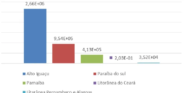
Figure 5. CF results – ACV (day.m3_.kgP-1_).

Alto Iguaçu and Paraíba do Sul presented the highest CF of all subwatersheds, consequently the

same amount of emitted phosphorus results in values of eutrophication potential higher at these

regions than in others.

Because of this high eutrophication potential there is concentration of hypereutrophy water

bodies at these watersheds.

4 CONCLUSIONS

The proposed goal was achieved through the LCIA method of freshwater eutrophication that

was regionalized promoting the first CF to estimate the eutrophication impact at Brazilian

subwatersheds.

This is the first study that presents a regionalized model to estimate Brazilian CF for freshwater

eutrophication. The regionalization was based on the models proposed by Helmes et al. (2012)

and Azevedo et al. (2013), which are considered the most complete and suitable models.

Due to the lack of data it was possible to calculate the CF for Alto Iguaçu micro watershed and

four subwatersheds: Paraíba do Sul, Parnaíba, Litorânea do Ceará and Litorânea Pernambuco

Alagoas. Among these watersheds, Alto Iguaçu has the highest CF.

The processes assessment of advection, retention and water use provides valuable information of

each region and also results in more realistic FF, since Brazilian sanitation is completely uneven,

and the sewage treatment must be modelled to not overestimated or sub estimated the FF.

to promote higher quality information, which can be used to make strategic decisions in order to

avoid eutrophication impact.

Finding the necessary data was the crucial part of the work because the lack of available data in

Brazil only considers the main rivers with low quality and low representativeness. To improve

the CF quality, is very important having data of affluent rivers, such as lakes and reservoirs.

Understanding the subwatershed, it becomes possible to direct financial resources to prioritize

preventives actions, such as sanitation and environmental education programs at regions as

Paraíba do Sul.

This was the first attempt to develop a Brazilian CF and some improvements need to be done.

Firstly, new studies ought to concentrate to promote good quality of data, then the regionalized

model should improve modeling treatment of industrial sewage and, finally, CF needs to be

calculated for all subwatershed.

ACKNOWLEDGEMENTS

We would like to express our gratitude to the CNPq for supporting this research.

Furthermore, we would like to thank the RAICV research group, the Life Cycle Sustainability

Assessment Center (Gyro) and the Profs. Laura and Tamara.

REFERENCES

AGÊNCIA NACIONAL DE ÁGUAS, [no date]. Indicadores de qualidade: Indicadores de estado trófico.

Portal da Qualidade das Águas [online]. [Accessed 1 January 2016]. Available from:

http://portalpnqa.ana.gov.br/indicadores-estado-trofico.aspx

ALEXANDER, R.B., SMITH, R.A. and SCHWARZ, G.E., 2004. Estimates of diffuse phosphorus sources in

surface waters of the United States using a spatially referenced watershed model. Water Science and

Technology. 1 February 2004. Vol. 49, no. 3, p. 1–10. DOI

10.2166/wst.2004.0150

.

ANDREOLI, Cleverson V. and CARNEIRO, Charles, 2005. Gestão integrada de mananciais de

abastecimento eutrofizados. Curitiba, PR: Sanepar; Finep.

AZEVEDO, Ligia B., HENDERSON, Andrew D., VAN ZELM, Rosalie, JOLLIET, Olivier and HUIJBREGTS,

Mark A. J., 2013. Assessing the Importance of Spatial Variability versus Model Choices in Life Cycle

Impact Assessment: The Case of Freshwater Eutrophication in Europe. Environmental Science &

Technology. 3 December 2013. Vol. 47, no. 23, p. 13565–13570. DOI

10.1021/es403422a

.

ESTEVES, Francisco de Assis, 1998. Fundamentos de limnologia. 2. Rio de Janeiro, RJ: Interciência.

EUROPEAN COMMISSION, JOINT RESEARCH CENTRE and INSTITUTE FOR ENVIRONMENT AND

SUSTAINABILITY, 2011a. International Reference Life Cycle Data System (ILCD) handbook: framework

and requirements for life cycle impact assessment models and indicators. Luxembourg: Publications

EUROPEAN COMMISSION, JOINT RESEARCH CENTRE and INSTITUTE FOR ENVIRONMENT AND

SUSTAINABILITY, 2011b. International reference life cycle data system (ILCD) handbook:

Recommendations for Life Cycle Impact Assessment in the European context. Luxembourg:

Publications Office.

GALLEGO, Alejandro, RODRÍGUEZ, Luis, HOSPIDO, Almudena, MOREIRA, María Teresa and FEIJOO,

Gumersindo, 2010. Development of regional characterization factors for aquatic eutrophication. The

International Journal of Life Cycle Assessment. January 2010. Vol. 15, no. 1, p. 32–43. DOI

10.1007/s11367-009-0122-4

.

HELMES, Roel J. K., HUIJBREGTS, Mark A. J., HENDERSON, Andrew D. and JOLLIET, Olivier, 2012.

Spatially explicit fate factors of phosphorous emissions to freshwater at the global scale. The

International Journal of Life Cycle Assessment. June 2012. Vol. 17, no. 5, p. 646–654. DOI

10.1007/s11367-012-0382-2

.

KRAMER, Rafael Duarte, 2012. Bacia hidrográfica do Alto Iguaçu: caracterização física e química e

determinação de diclofenaco, ibuprofeno e paracetamol [online]. Dissertação (Mestrado em Ciência e

Tecnologia Ambiental). Curitiba, PR: Universidade Tecnológica Federal do Paraná. [Accessed 4 May

2020]. Available from:

http://repositorio.utfpr.edu.br:8080/jspui/handle/1/501

ROSENBAUM, Ralph K., MARGNI, Manuele and JOLLIET, Olivier, 2007. A flexible matrix algebra

framework for the multimedia multipathway modeling of emission to impacts. Environment

International. 1 July 2007. Vol. 33, no. 5, p. 624–634. DOI

10.1016/j.envint.2007.01.004

.

SEPPÄLÄ, Jyri, POSCH, Maximilian, JOHANSSON, Matti and HETTELINGH, Jean-Paul, 2006.

Country-dependent Characterisation Factors for Acidification and Terrestrial Eutrophication Based on

Accumulated Exceedance as an Impact Category Indicator (14 pp). The International Journal of Life

Cycle Assessment. 1 November 2006. Vol. 11, no. 6, p. 403–416. DOI

10.1065/lca2005.06.215

.

TUNDISI, José Galizia, TUNDISI, Takako Matsumura and SIAGIS GALLI, Corina, 2006. Reservatórios da

Região Metropolitana de São Paulo: consequências e impactos da eutrofização e perspectivas para o

gerenciamento e recuperação. In: Eutrofização na América do Sul: causas, conseqüências e

tecnologias de gerenciamento e controle. IIE; IIEGA; ABC; IAP, Iana. p. 161–182.

UGAYA, Cássia Maria Lie, ALMEIDA NETO, José Adolfo de, FIGUEIREDO, Maria Cléa Brito de,

OLIVEIRA, Jéssyca Mariana de and UGAYA, Cássia Maria Lie (eds.), 2019. Eutrofização em água doce.

In: Recomendação de modelos de Avaliação de Impacto do Ciclo de Vida para o Contexto Brasileiro

[online]. Brasília, DF: Ibict. [Accessed 25 April 2020]. Available from:

http://acv.ibict.br/wp-

content/uploads/2019/07/Relat%C3%B3rio-de-Recomenda%C3%A7%C3%B5es-de-Modelos-de-Avalia%C3%A7%C3%A3o-de-Impacto-para-o-Contexto-Brasileiro.pdf

UGAYA, Cássia Maria Lie, 2016. Avaliação de Impacto do Ciclo de Vida: método para análise da

regionalização de fatores de caracterização. In: Anais do V Congresso Brasileiro em Gestão do Ciclo de

Vida. Fortaleza, CE: Embrapa; ABCV; UTFPR. 2016.

UNITED NATIONS ENVIRONMENT PROGRAMME, 2019. Global Guidance on environmental life cycle

APPENDIX I

• Paraiba do Sul subwatershed

Paraiba do Sul is located on the border of São Paulo, Rio de Janeiro and Minas Gerais, where around 1,966,728 inhabitants live (HÍDRICO, 2016). It is located at a tropical altitude zone, and the average temperature is from 17°C to 22°C (MMA/ANA). Paranaiba River is the main stem and it is connected to Bacia Grande and Bacia Doce watersheds.

• FF calculation

Applying the Subwatershed model FF takes 35.89 days. The process calculations are detailed below. o Calculation of 𝑘𝑎𝑑𝑣,𝑖

The income rate by advection was estimated for Preto (Bacia Doce watershed) and Pomba River (Bacia Grande watershed) and the total advection rate is 5.63 10-3 _days-1_{, which is the sum of the rate of both rivers.}

The main stem water flow rate was collected just before it disembogues in the Paraiba do Sul watershed. The water volume at Paraiba do Sul was estimated by the same process as Alto Iguaçu’s water volume.

Variables 𝑘𝑎𝑑𝑣,𝐺𝑟𝑎𝑛𝑑𝑒 𝑄𝐺𝑟𝑎𝑛𝑑𝑒 𝑉𝑡𝑜𝑡,𝐺𝑟𝑎𝑛𝑑𝑒 𝐴𝐺𝑟𝑎𝑛𝑑𝑒 𝑃𝐺𝑟𝑎𝑛𝑑𝑒 Meaning Income rates by advection of Bacia Grande subwatershed

Preto river flow rate at the spring of Bacia Grande watershed Total water volume of Bacia Grande subwatershed Water surface area of Bacia Grande subwatershed Average depth of Preto river

Units day-1 _m3_{/day m}3 _m2 _m

Value 1.13 10-3 _{7.89 10}6 _{6.96 10}9 _{4.64 10}9 _1.5 Source Calculated by the equation 2 𝑘𝑎𝑑𝑣,𝑖= 𝑄𝑖 𝑉𝑡𝑜𝑡,𝑖 (ATLAS DAS AGUAS, 2016) Calculated by the equation below 𝑉𝑡𝑜𝑡,𝑖 = 𝐴𝑡𝑜𝑡,𝑖 . 𝑃𝑡𝑜𝑡,𝑖 (DISPONIBILIDAD E HIDRICA, 2016) (CPRJ, 2016) Qualitative analysis Year/Period - From 1950 to ₂₀₀₉ - 2016 2006 Especial

differentiation - River - River, lake and reservoir River

Representativeness -

Low

(only the mean river water flow is considered)

- Medium (Reservoir isn’t considered)

Medium (Average depth is considered)

Method - Average - Sum Average

Available region - Paraíba _subwatershed - Brazil Bacia _subwatershed Grande

Variables 𝑘𝑎𝑑𝑣,𝐷𝑜𝑐𝑒 𝑄𝐷𝑜𝑐𝑒 𝑉𝑡𝑜𝑡,𝐷𝑜𝑐𝑒 𝐴𝐷𝑜𝑐𝑒 𝑃𝐷𝑜𝑐𝑒 𝑘𝑎𝑑𝑣,𝑇𝑂𝑇 Meaning Income rates by advection of Bacia Doce subwatershed Pomba river flow rate at the spring of Parnaiba do Sul watershed Total water volume of Bacia Grande subwatershed Water surface area of Bacia Doce subwatershed Average depth of Pomba river Total income rates by advection

Units day-1 _m3_{/day m}3 _m2 _{m day}-1

Value 4.5 10-3 _{3.58 10}6 _{7.95 10}8 _{5.3 10}8 _{1.5 5.63 10}-3_.

Source Calculated by _{the equation 2} (ATLAS DAS _{AGUAS, 2016)}

Calculated by the equation below 𝑉𝑡𝑜𝑡,𝑖 = 𝐴𝑡𝑜𝑡,𝑖 . 𝑃𝑡𝑜𝑡,𝑖 (DISPONIBILI DADE HIDRICA, 2016) (CPRJ, 2006) 𝑘𝑎𝑑𝑣,𝑇𝑂𝑇 = 𝑘𝑎𝑑𝑣,𝐵𝐺 + 𝑘𝑎𝑑𝑣,𝐵𝐷 Qualitative analysis Year/Period - From 1950 to ₂₀₀₉ - 2016 2006 - Especial

differentiation - River - River, lake and reservoir River -

Representativeness - Low (only the mean river water flow is considered) - Medium (Reservoir isn’t considered) Medium (Average depth is considered) -

Method - Average - Sum -

o Calculation of 𝑘𝑟𝑒𝑡,𝑗

𝑘𝑟𝑒𝑡,𝑗 is 3.4 10-4days-1. Water volume data of Paraíba do Sul is available. P removal rate at rivers is 0.012 day-1 because Parnaíba do Sul flow rate is higher than 14.55 m3_{/s(ALEXANDER et al., 2004).}

Variables 𝑘𝑟𝑒𝑡,𝑃𝑅 𝑉𝑡𝑜𝑡,𝑃𝑅 𝑘𝑟𝑒𝑡, 𝑟𝑖𝑣,𝑃𝑅 𝑉𝑟𝑖𝑣,𝑃𝑅

Meaning Outcome rates by retention of Parnaiba do Sul subwatershed

Total water volume of Parnaiba do Sul subwatershed Removal rate of phosphorus Parnaiba do Sul River Parnaiba do Sul River volume

Units day-1 _km3 _day-1 _km3

Value 3.4 10-4 _{5.12 0.012 1.44 10}-1

Source

Calculated by the equation 3 𝑘𝑟𝑒𝑡,𝑗

= 1

𝑉𝑡𝑜𝑡,𝑗

(𝑉𝑟𝑖𝑣,𝑗 . 𝑘𝑟𝑒𝑡, 𝑟𝑖𝑣,𝑗 + 𝑣𝑓. (𝐴𝑙𝑎𝑘,𝑗+ 𝐴𝑟𝑒𝑠,𝑗))

(BOLETIM, 2016) (ALEXANDER et _{al., 2004)}

Calculated by the equation below 𝑉𝑡𝑜𝑡,𝑖 = 𝐴𝑡𝑜𝑡,𝑖 . 𝑃𝑡𝑜𝑡,𝑖 Qualitative analysis Year/Period - 2016 2004 - Especial

differentiation - River, lake and reservoir

River

- Representativenes

s - High (Estimated by GIS)

Low

(The same rate for all regions) -

Method - Sum Average -

Available region - Paraíba _watershed do Sul Global -

Variables 𝐴𝑟𝑖𝑣,𝐼 𝑃𝑟𝑖𝑣,𝐼 𝑣𝑓 𝐴𝑙𝑎𝑘,𝐴𝐼

Meaning Water surface area of _{Parnaiba do Sul River}

Average depth of Parnaiba do Sul River Phosphorus uptake velocity at Parnaiba do Sul subwatershed

Lake and Reservoir surface area at Parnaiba do Sul subwatershed

Units km2 _{km km·day}-1 _km2

Value 9.58 10-2 _{1.5 10}-3 _{3.80 10}-5 _{4,29 10}-1

Source (DISPONIBILIDADE _{HIDRICA, 2016)} (CRPJ, 2006) (ALEXANDER et al., ₂₀₀₄₎ (DISPONIBILIDADE _{HIDRICA, 2016)} Qualitative analysis

Year/Period 2016 2006 2004 2016

Especial

differentiation River River River Lake

Representativeness High _{(Estimated by GIS)} Medium (Average depth is considered)

Low

(The same rate for all regions)

High

(Estimated by GIS)

Method Sum Average Average Sum

o Calculation of 𝑘𝑢𝑠𝑒,𝑗

It is -1,44 10-2_day -1 _{and it is calculated by the equation 7. The same assumptions used at Alto Iguaçu about domestic effluent} and particulate phosphorus are applied to Paraíba do Sul. The outcome rate by advection is estimated at the last station at the basin in São João da Barra city.

Variables 𝒌𝒖𝒔𝒆 𝒅𝒐𝒎,𝒋 𝑓𝑊𝑇𝐴,AI: 𝒇𝑫𝑰𝑻𝑾 𝒅𝒐𝒎,𝑱 𝒌𝒂𝒅𝒗,𝒋 𝒇𝑻𝑺

Meaning

Income rate of P by water used for domestic purpose at Paraíba do Sul subwatershed Fraction of water returned to downstream grid after being used for domestic sector at subwatershed.

Share of the total water use that is used for domestic purposes at Paraíba do Sul subwatershed Outcome rate by advection of Paraíba do Sul subwatershed Fraction of P removed by sewage treatment.

Units day-1 _{Dimensionless Dimensionless m}3_{/day Dimensionless}

Value -1,13 10-2 _{0.8 0.55 1.89 10}-2 _0.26 Source Calculated by the equation 9 𝑘𝑢𝑠𝑒 𝑑𝑜𝑚,𝑗 = 𝑓𝑊𝑇𝐴,𝐽 . 𝑓𝐷𝐼𝑇𝑊 𝑑𝑜𝑚,𝐽. 𝑘𝑎𝑑𝑣,𝑗 . (𝑓𝑇𝑆 − (1 − 𝑓𝑁𝑇𝑆)) (SPERLING M., VON, 1996) (ABASTECIMEN TO URBANO, 2016) Calculated by the equation 5 𝑘𝑎𝑑𝑣,𝑗 = 𝑄𝑗 𝑉𝑡𝑜𝑡,𝑗 It is calculated by the equation 10 𝑓𝑇𝑆= 𝑡. 𝑟 Qualitative analysis Year/Period - 1996 2016 - - Especial

differentiation - River subwatershed - -

Representativen

ess -

Low

(The same rate for all regions)

High

(Estimated by

GIS) - -

Method - Average Sum - -

Available region - Global Alto _subwatershed Iguaçu - -

Variables 𝒕 𝒓 𝒇𝑵𝑻𝑺 𝒅 𝑪𝑷 𝒓𝒊𝒗𝒆𝒓 𝑪𝑷 𝑻𝑺 Meaning Percentage of treated sewage at Paraíba do Sul subwatershed Percentage of phosphorus removed at effluent treatment Fraction of P transferred to the water body by dumping non-treated sewage Fraction of P at non- treated sewage P concentration at Paraíba river P concentration at treated sewage Units Dimensionless Dimensionle_ss Dimensionless Dimensionless mg/L mg/L

Value 0.37 0.71 -0.62 -0.98 0.087 14

Source (TRATA BRASIL, ₂₀₁₆₎ (CONAMA, ₂₀₁₁₎

It is calculated by the equation 11 𝑓𝑁𝑇𝑆 = (1 − 𝑡). 𝑑 Calculated by the equation below. 𝑑 =(𝐶𝑃 𝑟𝑖𝑣𝑒𝑟− 𝐶𝑃 𝑇𝑆) 𝐶𝑃 𝑇𝑆 (PGRH, 2016) (CONAMA, ₂₀₁₁₎ Qualitative analysis Year/Period 2016 2011 - - 2016 2011 Especial

differentiation Paraíba do Sul subwatershed Brazil - - Paraíba river Brazil Representative ness Medium (Percentage estimate of treated sewage) Low (The same rate for all regions) - - Low (Average of 3 samples) Low

(The same rate for all regions)

Method Average Average - - Average Average

Available

Variables 𝒌𝒖𝒔𝒆 𝒊𝒓𝒓𝒊𝒈,𝒋 𝒇𝑾𝑻𝑨,𝑱 𝒇𝑫𝑰𝑻𝑾 𝒊𝒓𝒓𝒊,𝑱 𝒇𝒔𝒐𝒊𝒍,𝑱 𝑅 𝒌 𝑻𝑶𝑻,𝒋 Meaning Outcome rate of P by water used for domestic purpose at Paraíba do Sul subwatershe d Fraction of water that returns to the waterbody after domestic use

Share of the total water use that is

used for irrigation at Paraíba do Sul subwatershed Fraction of total phosphorus emissions transferred at Paraíba do Sul subwatershed Runoff rate at Paraíba do Sul subwatershed Income rate of P by water used at Paraíba do Sul subwatershe d

Units day-1 Dimensionles

s Dimensionless Dimensionless mm.year-1 day-1

Value -1.27 10-2 _{0.8 0.23 4.62 596.38 2.40 10}-2 Source 𝑘𝑢𝑠𝑒 𝑖𝑟𝑟𝑖𝑔,𝑗 = 𝑓𝑊𝑇𝐴,𝐽 . 𝑓𝐷𝐼𝑇𝑊 𝑖𝑟𝑟𝑖,𝐽. 𝑘𝑎𝑑𝑣,𝑗 . (1 − 𝑓𝑠𝑜𝑖𝑙,𝐽) (SPERLING M., VON, 1996) (IRRIGAÇÃO, 2016) Calculated summing the equations 8 and 9 𝑓𝐷𝐼𝑃 = 0.29 (1 + (_0.85𝑅 ) −2 ) 𝑓𝐷𝑂𝑃= 0.01. 𝑅0.95 (ATALAS,2016 ) Calculated by the equation below. 𝑘 𝑇𝑂𝑇,𝑗 = |𝑘𝑢𝑠𝑒 𝑑𝑜𝑚,𝑗| − 𝑘𝑢𝑠𝑒 𝑖𝑟𝑟𝑖𝑔,𝑗 Qualitative analysis Year/Period - 1996 2016 - 1950-2000 - Especial

differentiation - River subwatershed - 0.5°x0.5° -

Representativen

ess -

Low (The same rate for all regions)

High

(Estimated by GIS)

- High -

Method - Average Sum - Average -

Available region - Global Alto _subwatershed Iguaçu - Global -

• EF calculation

TP concentration is measured between Santa Branca and the Paraíba River base level. The coefficients α and β are used to analyze stream water, because the rivers watershed volume is more representative than the lake and reservoir volumes.

Variables 𝑃𝑁𝑂𝐹𝐴𝐼: 𝐶𝐴𝐼: α β

Meaning Potentially non-_{occurring fraction}

TP concentration at Paraíba do Sul subwatershed

Species sensitivity distributions Slope of the PNOF TP function at lake

Species sensitivity distributions

Slope of the PNOF TP function in steam water

Units Dimensionless kg .m-3 _{Dimensionless Dimensionless}

Value 0.96 8.73 10-5 _{-3,13 0,426}

Source

Calculated using the equation

𝑃𝑁𝑂𝐹𝐴𝐼

= 1

1 + 𝑒𝑥𝑝−(𝑙𝑜𝑔𝐶0.63𝐴𝐼+0.54)

(PGRH, 2016) (AZEVEDO at al,. _2013b) (AZEVEDO at al,. 2013b)

Qualitative analysis

Year/Period - 2016 2013 2013

Especial

differentiation - River 0.5°x0.5° 0.5°x0.5°

Representativene

ss - Medium Low Low

Method - Average Average Average

Available region - Alto Iguaçu Europe Europe

• CF calculation

Variables 𝐴𝐸𝐹𝑗 𝑀𝐸𝐹𝑗 𝐿𝐸𝐹𝑗

Meaning Average effect factor Marginal effect factor Linear effect factor

Units m3 _{. kg P}1− _m3 _{. kg P}1− _m3 _{. kg P}1−

Value 1.10 104 _{4.05 10}2 _{6.74 10}2

Source

Calculated by the equation 𝐴𝐸𝐹𝐴𝐼=

𝑃𝑁𝑂𝐹𝐴𝐼 𝐶𝐴𝐼

Calculated by the equation 𝑀𝐸𝐹𝐴𝐼 = 𝑃𝑁𝑂𝐹𝐴𝐼 . (1 − 𝑃𝑁𝑂𝐹𝐴𝐼). 1 𝐶𝐴𝐼. 𝛽. ln (10) Calculated by the equation 𝐿𝐸𝐹𝐴𝐼= 0.5 10𝛼 Variables 𝐴𝐶𝐹𝐽 𝑀𝐶𝐹𝐽 𝐿𝐶𝐹𝐽

Meaning CF calculated by the AEF _model CF calculated by the MEF model CF calculated by the _{LEF model}

Units -day day day

Value 8.30 10-5 _{3.25 10}4 _{5,41 10}4

Source 𝐶𝐹 = 𝐹𝐹 . 𝐸𝐹- 𝐶𝐹 = 𝐹𝐹 . 𝐸𝐹 𝐶𝐹 = 𝐹𝐹 . 𝐸𝐹

• Parnaiba subwatershed

Parnaiba is located at the northeast of Brazil and in a megathermal rainy zone, which has an average temperature from 16º C to 32° C. Approximately 4.152.865 inhabitants live in this region. Parnaiba subwatershed is not connected to any subwatersheds, because all the rivers spring at the subwatershed. Therefore, the income rate by advection is zero.

• FF calculation

Applying the Subwatershed model FF takes 31.10 days. The process calculations are detailed below. o Calculation of 𝑘𝑟𝑒𝑡,𝑗

The water volume at Parnaíba was calculated the same way as Alto Iguaçu. The flow rate of Parnaíba River is base level so the removal rate of phosphorus is 0.012 day-1_{(ALEXANDER et al., 2004).}

Variables 𝒌𝒓𝒆𝒕,𝒋 𝑽𝒕𝒐𝒕,𝒋 𝑨𝒋 𝑷𝒋 𝒌𝒓𝒆𝒕, 𝒓𝒊𝒗,𝒋

Meaning Outcome retention of Parnaiba rates by subwatershed

Total water volume of Parnaiba subwatershed

Water surface area of Parnaiba subwatershed Average depth of Parnaiba River Removal rate of phosphorus of Parnaiba subwatershed

Units day-1 _km3 _km2 _{km day}-1

Value 9.52 10-3 _{5.64 1.11 10}3 _{5.09 10}-3 _0.012 Source Calculated by the equation 3 𝑘𝑟𝑒𝑡,𝑗 = 1 𝑉𝑡𝑜𝑡,𝑗 (𝑉𝑟𝑖𝑣,𝑗 . 𝑘𝑟𝑒𝑡, 𝑟𝑖𝑣,𝑗 + 𝑣𝑓. (𝐴𝑙𝑎𝑘,𝑗+ 𝐴𝑟𝑒𝑠,𝑗)) Calculated by the equation below. 𝑉𝑡𝑜𝑡,𝑗 = 𝐴𝑗 . 𝑃𝑗 (BOLETIM,2016) (CPRJ, 2006) ALEXANDER et al, 2004 Qualitative analysis Year/Period - - 2016 2006 2004 Especial

differentiation - - River, reservoir lake and River River

Representativen ess - - High (Estimated by GIS) Medium (Average depth is considered) Low

(The same rate for all regions)

Method - - Sum Average Average

Available region - - Brazil Parnaíba Global

Variables 𝑽𝒓𝒊𝒗,𝒋 𝑨𝒓𝒊𝒗,𝒋 𝑷𝒋 𝑣𝑓 𝑨𝒍𝒂𝒌,𝒋 𝑨𝒓𝒆𝒔,𝒋

Meaning Volume Parnaiba do Sul of River Water surface area of Parnaiba do Sul River Average depth of Parnaiba River Phosphorus uptake velocity at Parnaiba subwatersh ed Lake surface area of Parnaiba subwatershed Reservoir surface area of Parnaiba subwatershed Units km3 _km2 _{km km·day}-1 _km2 _km2 Value 2.55 5.02 102 _{5.09 10}-3 _{3.80 10}-5 _{2.37 10}2 _{3.69 10}2 Source Calculated by the equation below. 𝑉𝑟𝑖𝑣,𝑗 = 𝐴 𝑟𝑖𝑣,𝑗 . 𝑃𝑗 (DISPONIBILID ADE HIDRICA, 2016) (CPRJ, 2006) (ALEXANDE R et al., 2004) (DISPONIBILID ADE HIDRICA, 2016) (DISPONIBILID ADE HIDRICA, 2016) Qualitative analysis Year/Period - 2016 2006 2004 2016 2016 Especial

differentiation - River River River Lake Reservoir

Representative ness - High (Estimated by GIS) Medium (Average depth is considered) Low (The same rate for all regions) High (Estimated by GIS) High (Estimated by GIS)

Method - Sum Average Average Sum Sum

Available

Calculation of 𝑘𝑢𝑠𝑒,𝑗

𝑘𝑢𝑠𝑒,𝑗 is -1.18 10-3day-1and it is calculated by the equation 7. The same consideration made for Alto Iguaçu is used for Parnaíba subwatershed. Variables 𝒌𝒖𝒔𝒆 𝒅𝒐𝒎,𝒋 𝒇𝑾𝑻𝑨,𝐣: 𝒇𝑫𝑰𝑻𝑾 𝒅𝒐𝒎,𝑱 𝒌𝒂𝒅𝒗,𝒋 𝒇𝑻𝑺 Meaning Removal rate by water use of Parnaiba subwatershed

Fraction of water that returns to the waterbody after domestic use

Share of the total water use that is used for domestic purposes at Paraíba do Sul subwatershed Removal rate by advection at Parnaiba subwatershed Fraction of P removed by sewage treatment.

Units day-1 _{Dimensionless Dimensionless day}-1 _{Dimensionless}

Value -1.83 10-3 _{0.8 0.31 4.83 10}-3 _0.15 Source Calculated by the equation 9 𝑘𝑢𝑠𝑒 𝑑𝑜𝑚,𝑗 = 𝑓𝑊𝑇𝐴,𝐽 . 𝑓𝐷𝐼𝑇𝑊 𝑑𝑜𝑚,𝐽. 𝑘𝑎𝑑𝑣,𝑗 . (𝑓𝑇𝑆 − (1 − 𝑓𝑁𝑇𝑆)) (SPERLING M., VON, 1996) (ABASTECIMEN TO URBANO, 2016) Calculated by the equation 5 𝑘𝑎𝑑𝑣,𝑗 = 𝑄𝑗 𝑉𝑡𝑜𝑡,𝑗 It is calculated by the equation 10 𝑓𝑇𝑆= 𝑡. 𝑟 Qualitative analysis Year/Period - 1996 2016 - - Especial

differentiation - River subwatershed - -

Representativen

ess -

Low

(The same rate for all regions)

High

(Estimated by

GIS) - -

Method - Average Sum - -

Available region - Global Alto _subwatershed Iguaçu - -

Variables 𝒕 𝒓 𝒇𝑵𝑻𝑺 𝒅 𝑪𝑷 𝒓𝒊𝒗𝒆𝒓 𝑪𝑷 𝑻𝑺 Meaning Percentage of treated sewage at Parnaíba subwatershed Percentage of phosphorus removed at effluent treatment Fraction of P transferred to the water body by dumping non-treated sewage Fraction of P non- treated sewage P concentration at Parnaíba river P concentration at non-treated sewage Units Dimensionless Dimensionle_ss Dimensionless Dimensionless mg/L mg/L

Value 0.21 0.71 -0.66 -0.83 0.08 14

Source (TRATA ₂₀₁₆₎ BRASIL, (CONAMA, ₂₀₁₁₎

It is calculated by the equation 11 𝑓𝑁𝑇𝑆 = (1 − 𝑡). 𝑑 Calculated by the equation below. 𝑑 =(𝐶𝑃 𝑟𝑖𝑣𝑒𝑟− 𝐶𝑃 𝑇𝑆) 𝐶𝑃 𝑇𝑆 (INCT, 2016) (CONAMA, ₂₀₁₁₎ Qualitative analysis Year/Perio d 2016 2011 - - 2016 2011 Especial differentiat ion Parnaíba

subwatershed Brazil - - Paraíba river Brazil

Represent ativeness Medium (Percentage estimate of treated sewage) Low (The same rate for all regions)

- - Low (Average of 3

samples)

Low

(The same rate for all regions)

Method Average Average - - Average Average

Variables 𝒌𝒖𝒔𝒆 𝒊𝒓𝒓𝒊𝒈,𝒋 𝒇𝑾𝑻𝑨,𝑱 𝒇𝑫𝑰𝑻𝑾 𝒊𝒓𝒓𝒊,𝑱 𝒇𝒔𝒐𝒊𝒍,𝑱 𝑅 𝒌 𝑻𝑶𝑻,𝒋 Meaning Income rate of P by water used for domestic purpose at Parnaíba subwatershed Fraction of water that returns to the waterbody after domestic use

Share of the total water use that is used for irrigation at Parnaíba subwatershed Fraction of total phosphorus emissions transferred at Parnaíba subwatershed Runoff rate at Parnaíba subwatershe d Income rate of P by water used at Parnaíba subwaters hed

Units day-1 _{Dimensionless Dimensionless Dimensionless mm.year}-1 _day-1

Value -4.57 10-3 _{0.8 0.58 3.05 371.39 - 6.41 10}-3 Source 𝑘𝑢𝑠𝑒 𝑖𝑟𝑟𝑖𝑔,𝑗 = 𝑓𝑊𝑇𝐴,𝐽 . 𝑓𝐷𝐼𝑇𝑊 𝑖𝑟𝑟𝑖,𝐽. 𝑘𝑎𝑑𝑣,𝑗 . (1 − 𝑓𝑠𝑜𝑖𝑙,𝐽) (SPERLING M., VON, 1996) (IRRIGAÇÃO, 2016) Calculated summing the equations 8 and 9 𝑓𝐷𝐼𝑃 = 0.29 (1 + (_0.85𝑅 ) −2 ) 𝑓𝐷𝑂𝑃 = 0.01. 𝑅0.95 (ATALAS,201 6) Calculate d by the equation below. 𝑘 𝑇𝑂𝑇,𝑗 = |𝑘𝑢𝑠𝑒 𝑑𝑜𝑚,𝑗| − 𝑘𝑢𝑠𝑒 𝑖𝑟𝑟𝑖𝑔,𝑗 Qualitative analysis Year/Period - 1996 2016 - 1950-2000 - Especial

differentiation - River subwatershed - 0.5°x0.5° -

Representativen

ess -

Low

(The same rate for all regions) High (Estimated by GIS) - High (Estimated by GIS) -

Method - Average Sum - Average -

Available region - Global Alto _subwatershed Iguaçu - Global -

• EF calculation

TP concentration is the average value measured between March and August 2010.

Variables 𝑷𝑵𝑶𝑭𝒋 𝐶𝑗 α β

Meaning Potentially _fraction non-occurring TP concentration at Parnaíba River Coefficient α of _streams Coefficient β of streams

Units Dimensionless kg .m3 _{Dimensionless Dimensionless}

Value 1 8,00 10-5 _{-3.13 0.426}

Source

Calculated by the equation 𝑃𝑁𝑂𝐹𝐴𝐼

= 1

1 + 𝑒𝑥𝑝−(𝑙𝑜𝑔𝐶0.63𝐴𝐼+0.54)

(INCT, 2016) (AZEVEDO et al, _2013b) (AZEVEDO et al, 2013b)

Qualitative analysis Year/Period - 2016 2013 2013 Especial differentiation - River 0.5°x0,5° 0.5°x0,5° Representativenes s - Low (Average of few samples) Low (European context) Low (European context)

Method - Average Average Average

• CF calculation

CF is calculated using three different EF models.

Variables 𝐴𝐸𝐹𝐴𝐼: 𝑀𝐸𝐹𝐴𝐼: 𝐿𝐸𝐹𝐴𝐼:

Meaning Average effect factor Marginal effect factor Linear effect factor

Units m3 _{. kg P}1− _m3 _{. kg P}1− _m3 _{. kg P}1−

Value 1.30 104 _{-5.13 10}2 _{6,74 10}2

Source

Calculated by the equation 𝐴𝐸𝐹𝑗=

𝑃𝑁𝑂𝐹𝑗 𝐶𝑗

Calculated by the equation 𝑀𝐸𝐹𝐴𝐼 = 𝑃𝑁𝑂𝐹𝐴𝐼 . (1 − 𝑃𝑁𝑂𝐹𝐴𝐼). 1 𝐶𝐴𝐼. 𝛽. ln (10) Calculated by the equation 𝐿𝐸𝐹𝐴𝐼= 0.5 10𝛼 Variables 𝐴𝐶𝐹𝐴𝐼: 𝑀𝐶𝐹𝐴𝐼: 𝐿𝐶𝐹𝐴𝐼:

Meaning CF calculated by the AEF _model CF calculated by the MEF model CF calculated by the LEF _model

Units -day day day

Value 4.04 105 _{-1.60 10}4 _{2.10 10}4

Source 𝐶𝐹 = 𝐹𝐹 . 𝐸𝐹- 𝐶𝐹 = 𝐹𝐹 . 𝐸𝐹 𝐶𝐹 = 𝐹𝐹 . 𝐸𝐹

• Litorânea do Ceará

Litorânea do Ceará is also located at the northeast of Brazil and is not connected with any subwatersheds. It is divided in five regions: Acaraú, Coreaú, Curú, Litoral and Metropolitana.

• FF calculation

Applying the Subwatershed model FF takes 5.00 days. The process calculations are detailed below. o Calculation of 𝑘𝑟𝑒𝑡,𝑗

Litorânea do Ceará (LC) 𝑘𝑟𝑒𝑡,𝑗 is 3,28 10-3 . Its water volume is calculated adding the volume average of each region, which is estimated multiplying the average percentage storage capacity by the maximum volume. Consequently, the water volume of LC subwatershed is 6,30 10-2 _km3_.

LC water flow rate is the sum of the average values of the five main stem flow rates (96,68m3_{/s). Therefore, the phosphorus} removal rate is 0.012 day-1_{(ALEXANDER et al., 2004). More details can be found at the table 4.}

The main stem volume is estimated using the shapefile of water availability.

Variables 𝒌𝒓𝒆𝒕,𝒋 𝑽𝒕𝒐𝒕,𝒋 𝒌𝒓𝒆𝒕, 𝒓𝒊𝒗,𝒋 𝑽𝒓𝒊𝒗,𝒋

Meaning

Outcome rates by retention of LC subwatershed

Total water volume of LC subwatershed

phosphorus removal rate LC

subwatershed Volume LC do Sul River

Units day-1 _km3 _day-1 _km3

Value 3.28 10-3 _{6,30 10}2 _{0.012 1.69 10}2 Source Calculated by the equation 3 𝑘𝑟𝑒𝑡,𝑗 = 1 𝑉𝑡𝑜𝑡,𝑗 (𝑉𝑟𝑖𝑣,𝑗 . 𝑘𝑟𝑒𝑡, 𝑟𝑖𝑣,𝑗 + 𝑣𝑓. (𝐴𝑙𝑎𝑘,𝑗+ 𝐴𝑟𝑒𝑠,𝑗))

(HIDRO, 2016) (ALEXANDER et al, ₂₀₀₄₎

Estimated by the water

flow rate. (DISPONIBILIDADE HIDRICA, 2016) Qualitative analysis Year/Period 2015 to 2016 2004 2009/2015 Especial

differentiation - River, lakes and reservoir River River

Representativen

ess -

Medium

(Mean water bodies are considered)

Low

(The same rate for all regions)

High

(Estimated by GIS)

Method - Sum Average Sum

Available region - LC subwatershed Global LC subwatershed

Variables 𝑣𝑓 𝑨𝒍𝒂𝒌,𝒋 𝑨𝒓𝒆𝒔,𝒋

Meaning Phosphorus uptake velocity _{at LC subwatershed} Lake surface area of LC _subwatershed Reservoir surface area of LC _subwatershed

Units km·day-1 _km2 _km2

Value 3.80 10-5 _{1.42 10}2 _{6.84 10}2

Source (ALEXANDER et al., 2004) (DISPONIBILIDADE HIDRICA, ₂₀₁₆₎ (DISPONIBILIDADE HIDRICA, 2016)

Year/Period 2004 2016 2016

Especial

differentiation River Lake Reservoir

Representativene ss

Low

(The same rate for all regions)

High

(Estimated by GIS) High (Estimated by GIS)

Method Average Sum Sum