Fast return path planning for agricultural autonomous terrestrial robot in a known field



Abstract—The agricultural sector is becoming more critical than ever in view of the expected overpopulation of the Earth. The introduction of robotic solutions in this field is an increasingly researched topic to make the most of the Earth's resources, thus going to avoid the problems of wear and tear of the human body due to the harsh agricultural work, and open the possibility of a constant careful processing 24 hours a day. This project is realized for a terrestrial autonomous robot aimed to navigate in an orchard collecting fallen peaches below the trees. When it receives the signal indicating the low battery, it has to return to the docking station where it will replace its battery and then return to the last work point and resume its routine. Considering a preset path in orchards with tree rows with variable length by which the robot goes iteratively using the algorithm D*. In case of low battery, the D* algorithm is still used to determine the fastest return path to the docking station as well as to come back from the docking station to the last work point. MATLAB simulations were performed to analyze the flexibility and adaptability of the developed algorithm. The simulation results show an enormous potential for adaptability, particularly in view of the irregularity of orchard field, since it is not flat and undergoes modifications over time from fallen branch as well as from other obstacles and constraints. The D* algorithm determines the best route in spite of the irregularity of the terrain. Moreover, in this work, it will be shown a possible solution to improve the initial points tracking and reduce time between movements.

Keywords—Path planning, fastest return path, agricultural terrestrial robot, autonomous, docking station.

I. INTRODUCTION

HE ability to navigate in a substantially easy way thanks to the current GPS systems, combined with other sensors that allow the improvement of traceability, as well as the evolution of artificial intelligence algorithms available, make this work possible without a great financial effort.

In this work of path planning, we start by knowing the path that the robot will have to follow to navigate the field. This is possible because the first time, the robot follows the defined path thanks to a "manual" guide; at this point, the robot samples the positions taken during its journey with a fixed frequency, "saving" various check points in succession.

C. Cernicchiaro is with the University of Beira Interior, Rua Marquês d’Ávila e Bolama, 6201-001, Covilhã, Portugal and University of Modena and Reggio Emilia, via Amendola 2 - Pad. Morselli, 42122 - Reggio Emilia (e-mail: 231268@studenti.unimore.it).

P. D. Gaspar is with the University of Beira Interior, Rua Marquês d’Ávila e Bolama, 6201-001, Covilhã, Portugal and C-MAST - Centre for Mechanical and Aerospace Science and Technologies (corresponding author; phone: (+351)275329759; e-mail: dinis@ubi.pt).

M. L. Aguiar is with the University of Beira Interior, Rua Marquês d’Ávila e Bolama, 6201-001, Covilhã, Portugal and C-MAST - Centre for Mechanical and Aerospace Science and Technologies (e-mail: martim_84@hotmail.com).

The route includes the departure from the dock station, positioned, ideally, in the point of origin of two perpendicular Cartesian axes that describes a 2D field; always remaining in this idealization, the field to be worked exists only in the first quadrant, i.e., the one in which both the x and y axes assume positive values. After the start, the robot places side-by-side the line of trees - parallel to the y axis, equidistant from each other and of the same length - first on one side and then on the other and, before moving on to the next line, the center of the lines. Doing so and avoiding passing through the trees, due to robot dimension, the vehicle is able to cover the entire field, ensuring the collection of all the peaches present on the ground. When the battery is about to discharge, a signal alerts the robot of the current condition and the algorithm calculates the shortest route back to the dock station. Once the recharge is complete, the robot will return to the last work point and continue its working routine until the battery is exhausted again.

In this work, the state-of-the-art algorithm covering the technology and the control will be explored first, and then the elaborated formula will be explained.

II. STATE OF THE ART

Recently, even in the field of agricultural crops, a good level has been achieved with route planning (i.e., finding the optimal route between two points avoiding obstacles), which is considered a common and obligatory aid activity for agricultural robots [1], [2].

It is also worth mentioning the important work developed with a 3D field coverage approach which allows a total coverage for each type of topographic structure of the field surface [2], [3]. Also, the autonomous guidance had some progress; in fact it has been used in the rice transplanter, determining position and orientation with GPS, sensors and optical fiber gyroscopic accelerometers (FOG) as well as rotary encoders and proximity sensors. The speed and orientation of the vehicle were controlled by the outputs of a PLC [2], [4].

An automatic driving system was developed on the basis of an RTK-GPS, thanks to which, a tractor was driven along pre-set routes. In this case, a special control law was designed for non-linear velocity [2], [5].

It was also developed an autonomous vehicle that had the task of inspecting the field while minimizing its influence on the harvest and soil compaction. Here, you can find a reflex camera that extracts the central culture line in uncontrolled lighting conditions, a camera with a GPS receiver, and two fuzzy controllers that give a guided visual navigation [2], [6].

Carlo Cernicchiaro, Pedro D. Gaspar, Martim L. Aguiar

Fast Return Path Planning for Agricultural

Autonomous Terrestrial Robot in a Known Field

T

It is useful to mention the development of the work carried out for the creation of an optimal path between two points having, among them, simple polygonal disjunctions [7], [8].

An algorithm was developed to drive an autonomous tractor equipped with an intelligent navigator [8], [9].

A dynamic model of bicycle approach is used to evaluate the trajectories of a tractor implementation system. This model was evaluated in MATLAB and tested in the field [4], [8].

An end-of-line turning algorithm was developed by creating two types of turning paths with the third-type spline function, forward and backward rotation. Finally, a power function has been introduced to calculate the maximum limit of the steering speed [8], [10].

A controller was designed to drive a robot tractor forward and backward, using a simplified bicycle model for the

kinematic model [8], [11].

To take into account the impact of machines on the ground, you can use the Semantical Occupancy Grid Maps (SOGM) [12]. Considering the shape of our field, a possible solution could be the solution which uses the union of Boustrophedon cellular decomposition and Chinese post problem [13]. To better understand this algorithm, it is necessary to discuss about the two algorithms used in this solution:

- The Boustrophedon cellular decomposition: This method transforms the configuration space into cell regions, allowing to cover these cells avoiding obstacles (as shown in Fig. 1). As can be seen, the robot follows the field just going back and forth sliding his path to the right (in this case).

Fig. 1 The Boustrophedon cellular decomposition [12]

- The Chinese Postman Problem: It consists in creating a cyclic path of minimum length in an undirected graph that crosses all its edges, as shown in Fig. 2. In an Eulerian graph, the solution is represented by an Eulerian path, and the shortest path length equals the number of arcs present.

Fig. 2 A representation of the Chinese Postman Problem.

- Optimal Coverage of a Known Arbitrary Environment: The first thing to do is to split the entire field using the Boustrophedon cellular decomposition, sweeping the bitmap. Without loss of generality, we assume a sweep direction along the x-axis and record all the critical

points/regions. During the sweep, the location of the cells is also recorded. Finally, the critical points and the cells are encoded in the Reeb graph. The resulting Reeb graph G =< V; E > is used as input to the next step of the algorithm that calculates an Euler tour.

It is possible doubling selected edges of the Reeb graph. Consequently, when the robot covers one of these doubled edges, it will split the cell into top and bottom sub-cells and assign each sub-cell to one of the two doubled edges.

The Euler tour (that is the routing of the robot) is: 𝑥 is integer 𝑒 ∈ 𝐸; 𝑤 is integer 𝑛 ∈ 𝑉;

𝑥 0, 𝑒 ∈ 𝐸; 𝑤 0, 𝑛 ∈ 𝑉; ∑ ∈ 𝑎 𝑥 2𝑤 𝑏 , 𝑛 ∈ 𝑉;

𝑧 ∑ ∈ 𝑐 𝑥 is minimized

𝑥 is the number of added copies of edge e in the solution. ∑ ∈ 𝑎 𝑥 represents the number of added edges to node 𝑛 ∈

𝑉 in the solution. Note that for the solution to be an Eulerian graph, an odd number of edges have to be added to nodes with odd degree and an even number of edges has to be added to nodes with even degree. 𝑏 is 1 for nodes with odd degree and 0 for nodes with even degree. 𝑤 is a variable that will force ∑ ∈ 𝑎 𝑥 to be odd for odd nodes and even for even nodes. 𝑎 is 1 if node n meets edge e, and 0 otherwise; is the cost of edge e. Given this notion, the proposed algorithm suggests to cover during the first traversal the left (or right) half of the cell, and in the second traversal to cover the right (or left) half of the cell, correspondingly (the same thing could be done in the top or bottom half of the cell; it depends if, respectively, the cell is free from obstacles or not). The choice of which half to cover is dictated by the position of the robot at the end of the previous coverage. It should give us a better control of the point of entry of the next cell. An example is shown in Fig. 3.

Fig. 3 Coverage of a single cell: depending on the number of up-down motions: (a) odd number, (b) even number

Another possible and easier solution could be the simple Boustrophedon cellular decomposition [14].

Fig. 4 Illustration of the explorer/coverer approach

When the low battery signal tells that it is time to go back to recharge, it is necessary to use an algorithm that finds the shortest route back to the dock station. One possible solution is to use the D* algorithm [14].

Using the D* algorithm, we describe the occupation map as a grid of costs where for cost c ∈ R, c > 0, we mean to cross each cell in a horizontal or vertical direction, while crossing the cell diagonally involves a cost of c=√2 and, in the final location, the cells have a cost c = ∞.

The purpose of the algorithm is to find the path that minimizes the total cost of the trip.

The main feature of this algorithm is that, thanks to it, it is possible to incrementally replace the cost of the cells, so as to model any changes in our map.

The D* algorithm is, basically, an evolution of A* algorithm; indeed, in this case, arc cost parameters can change

during the problem solving process.

The A* algorithm constructs multiple paths starting from a specific node. For each path, a cost is attributed which makes one or more of the others prefer. The algorithm therefore tends to minimize the function:

𝑓 𝑛 𝑔 𝑛 ℎ 𝑛

Having indicated with n the last node on the path, g(n) is the cost of the entire path from the initial node to node n, and

h(n) is a heuristic function that gives an estimate of the lowest

cost from n to target. The latter, in order for the algorithm to find the one that actually turns out to be the shortest route, must be admissible [14].

Upon returning to the dock station, the robot must be placed with high precision to ensure correct charging. A possible solution is to provide the dock station with 2 IR sensors able to detect the presence of obstacles; so that, when both detectors notice the presence of the robot, it will be sure that it is centered and, therefore, can start with parking maneuvers [15].

Fig. 5 (a) The robot is detected by one of the IR sensors. (b) The robot is detected by both sensors. (c) The robot turns 90 degrees to face the docking station. (d) The robot connects itself to the docking

station

III. THE ALGORITHM

Fig. 6 An example of basic map

To do this work, the Robotics Toolbox for MATLAB was used [15]. The work developed by [16], [17] was used to set the problem constraints. Firstly, the map was modeled imposing the tree line as straight lines, to avoid collisions and going through the tree line, as shown in Fig. 6. Then, we imposed the path to follow. For our purpose, we modeled the path in this way: starting from the assumptions that the robot must “walk” alongside the line of trees and at the center of the space between the lines, we have developed the path in such a way that, after having reached the first point, the y oscillates between y = ymin - 1 and y = ymax + 1 – where ymin and ymax represent, respectively, the minimum and maximum y of the line at two step intervals. The x is equal to xline-1-1, xline-1 + 1,

xline-1 + (xline-2-xline-1)/2 – where xline1 and xline2 are x coordinates

of two general consecutive lines, also increasing every two steps but starting off with one step from y; so that, alternately, each step only increases the coordinate x or just the coordinate

y.

According to the map in Fig. 1 (where ymin = 6, ymax = 30,

xline-n = 6n, with n ϵ N indicating the number of the tree line),

the path is described by the following two strings:

X = [1 5 5 7 7 9 9 11 11 13 13 15 15 17 17 19 19 21] Y = [1 5 31 31 5 5 31 31 5 5 31 31 5 5 31 31 5 5]

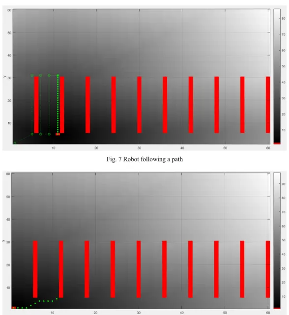
Then, a routine as prepared that lasts for the entire duration of tracking the points of the route. We have resorted to an iterative use of the D* algorithm to go from one point to another, as exemplified in Fig. 7.

To simulate the exhausted battery, a random number was generated, contained in a given range, at the beginning of the tracking routine. If the number coincides with a prefixed number, the program blocks the current routine and enters another subroutine that marks the dock station as a point of arrival. The return path example is shown in Fig. 8.

Fig. 7 Robot following a path

Fig. 8 Shortest comeback path to the dock station after signal of low battery is detected

When the robot detects a full battery, it comes back to the memory-stored coordinates when the low battery condition was determined, as shown in Fig. 9. After this, the robot goes to the point where it should be if the latter subroutine had not been triggered. It returns to the main routine where it will continue to follow the path until a new low battery signal arrives or until it finishes the points to be covered. An

example is shown in Fig. 10.

IV. RESULTS

The fast return path planning algorithm was tested to come back to the dock station from different positions. Figs. 11-14 exemplifies the results. Fig. 11 describes the path from the initial location [xi yi] = [10 10] to final location [xf yf] = [1 1],

and fast return to initial position after recharging.

Fig. 9 Returning to the last location after battery recharging

Fig. 10 Robot resumes its routine after recharge

(a) [xi yi] = [10 10] to [xf yf] = [1 1], t = 4.650598 s

(b) Path (a), modifying the cost map by adding 2 in the range x:4-8 and y:4-x:4-8. t = 3.605526 s

(c) [xi yi] = [1 1] to [xf yf] = [10 10], t = 3.485108 s

(d) Path (c), modifying the cost map by adding 2 in the range x:4-8 and y:4-x:4-8. t = 4.06011x:4-8 s

Fig. 11 Path from the initial location [xi yi] = [10 10] to final location

[xf yf] = [1 1], and fast return to initial position after recharging Fig. 12 describes the same process in a path starting from [xi

yi] = [20 20] and final location [xf yf] = [1 1], while Fig. 13

starts at [xi yi] = [40 30].

(a) [xi yi] = [20 20] to [xf yf] = [1 1], t = 3.418743 s

(b) Path (a), modifying the cost map by adding 2 in the range

x:19-21 and y:19-21. t = 3.182481 s

(c) [xi yi] = [1 1] to [xf yf] = [20 20], t = 3.340609s

(d) Path (c), modifying the cost map by adding 2 in the range

x:19-23 and y:4-19. t = 3.969876 s

Fig. 12 Path from the initial location [xi yi] = [20 20] to final location

[xf yf] = [1 1], and fast return to initial position after recharging

(a) [xi yi] = [40 30] to [xf yf] = [1 1], t = 3.868176 s

(b) Path (a), modifying the cost map by adding 2 in the range

x:37-39 and y:4-29. t = 3.305416 s

(c) [xi yi] = [1 1] to [xf yf] = [40 30], t = 3.524512s

(d) Path (c), modifying the cost map by adding 2 in the range

x:37-39 and y:4-29. t = 3.421170 s

Fig. 13 Path from the initial location [xi yi] = [40 30] to final location

[xf yf] = [1 1], and fast return to initial position after recharging

(a) [xi yi] = [55 15] to [xf yf] = [1 1], t = 3.181965 s

(b) Path (a), modifying the cost map by adding 2 in the range

x:55-58 and y:4-14. t = 3.303056 s

(c) [xi yi] = [1 1] to [xf yf] = [55 15], t = 3.638218 s

(d) Path (c), modifying the cost map by adding 2 in the range

x:55-58 and y:4-14. t = 3.534872 s

Fig. 14 Path from the initial location [xi yi] = [55 15] to final location

[xf yf] = [1 1], and fast return to initial position after recharging Table I shows the comparison of the elapsed time of the path between the robot actual position and the dock station.

TABLEI

ELAPSED TIME WHEN THE ROBOT GOES TO DOCK STATION AND COMES BACK TO WORK Tested Point Goes to the dock station Come back to work

Goes to the dock station (modifying

map cost)

Come back to work (modifying map cost) [10 10] 4.6506 s 3.4851 s 3.6055 s 4.0601 s [20 20] 3.4187 s 3.3406 s 3.1825 s 3.9699 s [40 30] 3.8682 s 3.5245 s 3.3054 s 3.4212 s [55 15] 3.182 s 3.6382 s 3.3031 s 3.5349 s

As is possible to see, the elapsed time varies within a time range of 3.182 s to 4.6506 s.

We estimated that the velocity to cross a cell is of 0.025 s per cell. This data has to be related with the mechanical characteristic of the chosen robot.

V. CONCLUSIONS

In this work, it was explored a solution for a robot with the task to move around an agriculture field. The purpose may be for taking photographs of the trees and/or fruits, to fertilize the soil, to spray herbicide, or other activity that may be included in the usual tasks to be performed in an orchard.

We assumed that the robot is able, thanks to its mechanical design, to overcome every kind of terrain. However, in real real orchards, the irregularity or inclination of the terrain may pose some restrictions to the rover locomotion despite its maneuverability. Thus, with the current algorithm there is the possibility to plan also the “not preferential” path to avoid. In fact, to simulate the irregular terrain, it is possible to change the difficulty to cross the wanted part of the terrain with the cost map modify command present in the D* algorithm.

Moreover, in order to overcome the time to calculate the path from one point to the other, it is possible to split the algorithm in two versions: one that calculates just the number of even points (p0, p2, p4, etc.) and the other just the odd points (p1, p3, p5, etc.), where, according to our example: p0 = [1, 1],

p1 = [5, 5], p2 = [31, 5] and so on; in this way, the program2

calculates the next path while the robot is going to its current goal – calculated by the program1 – and, when it reaches the current goal, program2 is already ready to perform the task and program1 can start to calculate the path to follow next.

ACKNOWLEDGMENT

This study is within the activities of project PrunusBot - Sistema robótico aéreo autónomo de pulverização controlada e previsão de produção frutícola (autonomous unmanned aerial robotic system for controlled spraying and prediction of fruit production), Operation n.º PDR2020-101-031358 (leader), Consortium n.º 340, Initiative n.º 140 promoted by PDR2020 and co-financed by FEADER under the Portugal 2020 initiative.

REFERENCES

[1] P. Bhattacharya and M. L. Gavrilova. “Roadmap-based path planning and Using the voronoi diagram for a clearance-based shortest path. Robotics & Automation Magazine”, pp. 58-66, 2008.

[2] A. Bechar, C. Vigneault, “Agricultural robots for field operations: Concepts and components”, Biosystems Engineering, 149, pp. 94-111, 2016.

[3] I. A. Hameed, A. la Cour-Harbo and O. L. Osen. “Side-to-side 3D coverage path planning approach for agricultural robots to minimize skip/overlap areas between swaths”, Robotics and Autonomous Systems, 76, pp. 36-45, 2016.

[4] Y. Nagasaka, N. Umeda, Y. Kanetai, K. Taniwaki and Y. Sasaki. “Autonomous guidance for rice transplanting using global positioning and gyroscopes”, Computers and Electronics in Agriculture, 43(3), pp. 223-234, 2004.

[5] B. Thuilot, C. Cariou, P. Martinet, and M. Berducat, “Automatic guidance of a farm tractor relying on a single CP-DGPS”, Autonomous Robots, 13(1), pp. 53-71, 2002.

[6] J. M. Bengochea-Guevara, J. Conesa-Mu~noz, D. Andu´ jar and A. Ribeiro. “Merge fuzzy visual servoing and GPS-based planning to obtain a proper navigation behavior for a small crop-inspection robot”, Sensors (Basel), 16(3), 2016.

[7] Z. Zhong-Xiang, C. Jun, Y. Toyofumi, T. Ryo, S. Zheng-he, M. En-rong, “Path tracking control of autonomous agricultural mobile robots”, Journal of Zhejiang University-SCIENCE A, 8(10), pp. 1596–1603, 2007.

[8] H. Mousazadeh, “A technical review on navigation systems of agricultural autonomous off-road vehicles”, Journal of Terramechanics, 50(3), pp. 211-232, 2013.

[9] Q. Zhang and H. Qiu, “A dynamic path search algorithm for tractor automatic navigation”, Transactions of ASAE, 47, pp. 639–46, 2004. [10] M. Kise, N. Noguchi, K. Ishii and H. Terao “Enhancement of turning

accuracy by path planning for robot tractor”, in Proc. of the Automation Technology for Off-Road Equipment Conference, Chicago, Illinois, USA, pp. 398–404, July 26-27, 2002.

[11] M. Kise, N. Noguchi, K. Ishii, H. Terao, “The development of the autonomous tractor with steering controller applied by optimal control”, in Proc. of the Automation Technology for Off-Road Equipment Conference, Chicago, Illinois, USA, pp. 367–73, July 26-27, 2002. [12] T. Korthals, M. Kragh, P. Christiansen, H. Karstoft, R. N. Jørgensen and

U. Rückert, “Multi-Modal Detection and Mapping of Static and Dynamic Obstacles in Agriculture for Process Evaluation”, Frontiers in Robot and AI, pp. 5-6, 2018.

[13] R. Mannadiar and I. Rekleitis, “Optimal Coverage of a Known Arbitrary Environment”, in Proc. of 2010 IEEE International Conference on Robotics and Automation, Anchorage, AK, USA, 3-7 May, 2010. [14] M. Rekleitis, A. P. New, E. S. Rankin, and H. Choset, “Efficient

Boustrophedon Multi-Robot Coverage: an algorithmic approach”, Annals of Mathematics and Artificial Intelligence, 52(2–4), pp 109–142, 2008.

[15] Peter Corke, “Robotics, Vision and Control - Fundamental Algorithms in MATLAB®”, Springer Tracts in Advanced Robotics Springer, 2011. [16] W. Zeng, R. L. Church, "Finding shortest paths on real road networks:

the case for A*", International Journal of Geographical Information Science, 23(4), pp. 531–543, 2009.

[17] G. Song, H. Wang, J. Zhang, and T. Meng, “Automatic docking system for recharging home surveillance robots”, IEEE Transactions on Consumer Electronics, 57(2), pp. 431-433, 2011.