Terry Carreiro Lima
UMinho|20
13
outubro de 2013
Mor
tgage Credit Default
: An empirical anal ysis of t he P or tuguese Mark e t
Escola de Economia e Gestão
Mortgage Credit Default:
An empirical analysis of the Portuguese Market
Terr
y Carr
eir
Dissertação de Mestrado
Mestrado em Economia Monetária, Bancária e Financeira
Trabalho efetuado sobre a orientação da
Professora Doutora Cristina Alexandra Oliveira Amado
Terry Carreiro Lima
outubro de 2013
Escola de Economia e Gestão
Mortgage Credit Default:
i
É AUTORIZADA A REPRODUÇÃO INTEGRAL DESTA DISSERTAÇÃO APENAS PARA EFEITOS DE INVESTIGAÇÃO, MEDIANTE DECLARAÇÃO ESCRITA DO INTERESSADO, QUE A TAL SE
COMPROMETE;
Universidade do Minho, ___/___/______
ii
Dedication
I dedicate this to Catarina Cabral, whose love, devotion, kindness and everything else kept me going and going towards my goals. She was my stable rock in the middle of the storm that was this thesis. More important, she is my home away from home. As long as I have her by my side, there is nothing impossible or improbable. As long as I have her by my side, I know that I have a place where I belong!
iii
Acknowledgements
First of all, I would like to thank my family and friends which supported me in this important phase of my academic life.
Second, I would like to thank Duarte Mendes Paiva, whose expertise in programming was an important factor in the realization and concretization of this work. He alone was able to mount and make sense of my rumbling ideas, turning them from nothing, to something.
In third place, I would like to thank Professor João Pedro Gonçalves, which precious help and knowledge led me in the right way and to a better understanding of financial options and the binomial model.
Next, Professor Gualter Couto, whose orientation and brief advice about Real Options was very helpful into better understanding the financial intricacies of options associated to real estate. Last, but not least, Professor Cristina Amado whose knowledge and advice where more than I could ever ask for to finish this thesis.
iv
RESUMO
O crédito hipotecário tornou-se numa das obrigações financeiras mais importantes das famílias portuguesas, mas por outro lado, este tipo de crédito tem sido capaz de aumentar alguns sectores económicos em Portugal. É importante estudar o incumprimento no crédito hipotecário, devido ao seu impacto sobre as famílias, e também sobre a banca e mercado imobiliário. O objetivo deste trabalho é duplo. Em primeiro lugar, utilizando um modelo de avaliação de opções, proponho calcular o preço da opção put e analisar se os donos de imóveis para habitação exerceram devido ao seu elevado valor. Em segundo lugar , vou usar um modelo VAR com variáveis macroeconómicas para analisar se estes afetam a actual taxa de incumprimento de crédito hipotecário, quando o valor da opção put não é elevado o suficiente para ser exercido. O principal resultado sugere que a opção put do investidor não era valioso o suficiente para justificar o seu exercício por parte deste. O estudo das variáveis macroeconómicas propostas levou-me à conclusão de que o PIB, a Poupança líquida , o Desemprego e a Volatilidade Imobiliária têm impactos negativos sobre Credit Default.
v
Abstract
Mortgage credit has become one of the most important, financial obligations of the Portuguese families, but on the other hand, this type of credit has been able to boost some economic sectors in Portugal. It is important to study default in the mortgage credit due to its impact on families, and also on the banking and real estate market. The aim of this work is twofold. Firstly, using an option pricing model, I propose to price the put option and analyze if the house owners exercised default due to a high put price. Secondly, I shall use a Vector Autoregressive model with macroeconomic variables to analyze if they affect the current rate of default when the put option is not valuable enough to be exercised. The main result suggests that the investor’s put option was not valuable enough to justify the exercising of his/her default option. Studying the proposed macroeconomic variables led me to the result that GDP, Net Savings, Unemployment and Real estate Volatility have negative impacts on Credit Default.
vi INDEX Dedications _______________________________________________________ ii Acknowledgements __________________________________________________ iii Resumo __________________________________________________________ iv Abstract __________________________________________________________ v Index ____________________________________________________________ vi List of Figures ______________________________________________________ viii List of Tables ______________________________________________________ ix
Section 1 ... 1
1. Introduction ... 1
Section 2 ... 3
2. Identification of the problem ... 3
2.1. Evolution of the Real estate market ... 3
Section 3 ... 6
3. Literature Review ... 6
3.1. Option Pricing Models ... 6
3.2. Analyzing the House Market Using Option Pricing Models ... 7
3.3. Pricing Methods ... 9
3.4. Mortgage default and macroeconomic variables ... 10
Section 4 ... 12
4. Empirical Analysis ... 12
4.1. Data ... 12
4.1.1. Modeling the Volatility of Real estate ... 14
4.2. Econometric Model ... 16
4.2.1. The Augmented Dickey-Fuller tests ... 17
4.2.2. The Kwiatkowski, Phillips, Schmidt, and Shin test ... 19
4.3. Granger Causality test ... 20
vii
4.5. Data for Binomial Model ... 22
4.6. Binomial Process ... 22 4.6.1. Backward Pricing ... 25 Section 5 ... 27 5. Empirical Results ... 27 5.1. Econometric Model ... 27 5.2. Options Model ... 28 Section 6 ... 30 6. Conclusions ... 30 References ... 32 Appendix ... 34 Figure A ... 34 Figure B ... 34 Figure C ... 35 Figure D ... 35 Figure E ... 36 Figure F ... 36 Figure G ... 37 Figure H ... 37 Figure I ... 38
viii
List of Figures
Figure 1: Evolution of the private consumption of the Portuguese families, between the first quarter of 2000, and
the last quarter of 2010, in 106 euros __________________________________________________ 4
Figure 2: Evolution of the unemployment rate in Portugal, between first quarter of 2000, and the last quarter of
2010 (in percentage) ______________________________________________________________ 4
Figure 3: Evolution of Doubtful Loans of other monetary financial institutions to individuals for housing purpose, in
106 euros ___________________________________________________________ 5
Figure 4: ACF and PACF for 30 lags __________________________________________ 15
Figure 5: Simulation using a Binomial lattice _____________________________________ 24
Figure 6: One state model ________________________________________________ 24
Figure 7:Computation of the put option at moment 41 _______________________________ 25
ix
List of Tables
Table 1: AR(p) models _________________________________________________ 15 Table 2: GARCH(1,1) test results __________________________________________ 16 Table 3: ADF test results _______________________________________________ 18 Table 4: KPSS test ____________________________________________________ 19 Table 5: F-test results from VAR model _____________________________________ 20 Table 6: Vector Autoregression Estimates ___________________________________ 21 Table 7: Initial Conditions _______________________________________________ 23 Table 8: Moments and Values ____________________________________________ 23 Table 9: Results for the value of the put option ________________________________ 29
1
1. Introduction
According to the Portuguese Banking Association (APB), 85% of the total of credit in 2011 to individuals was related to mortgage credit (Bolhetim Informativo Nº47, APB). This figure shows the increasing importance of real estate market on the current Portuguese economy, not only to individuals, but also to banks (as lenders) and the construction sector (responsible for house construction).
The increasing in credit concession for housing, and being it a long-term investment, the risk of defaulting is also associated. The expansion of mortgage credit also brought the burden of exposure to bad credit and the consequences of default. This type of credit has become one of the most costly financial obligations to families; see Fazenda (2008). Default happens when an individual or family has no financial liquidity to carry on the payments of the mortgage credit, turning over the possession of their house to the lenders for a complete financial pardon from there mortgage obligations. This can cause severe damage to lenders and compromise their ability to concede new credits, as well as problems in the real estate market concerning unexpected increase in volatility and supply in the market, affecting housing prices.
Housing acquisition through credit has become the most important investments by families. As any investor, their position in the investment has to be evaluated at every point of its existence. This means that the investor has a series of options that need to be priced during the investment, such that he/she understands his position and choose the most valuable option for him/her (either continue paying the financial obligations or default). Default is an option in any investment, and if this option is valuable enough for the investor, it will be exercised by the latter. The problem is the need to properly price the default option, and if this alternative is valuable, should the investor exercise it. If the default option is not valuable enough to be exercise, one may ask why are defaults occurring in the mortgage credit? Is the investor compromised by the economic environment, or are there any events that make the investor choose defaulting? The purpose of this thesis is to answer these questions. This shall be accomplished by using an option-model approach to price and compare options that the investor has, but also use a Vector Autoregressive model to measure the impact of some macroeconomic variables on the mortgage default phenomena.
2
Black and Scholes (1973) are the pioneers of pricing options using binomial models, and laydown the necessary framework and concepts to use in this type of models for pricing options on financial assets. Kau and Keenan (1992, 1995) use this model and apply it to specific cases of mortgage default. Also, they propose the best method for pricing the default option, i.e. the put option, and how to study default and prepayment as competing options. In this thesis, the building constructed for housing shall be the asset under study. Because the default option can be seen as a real option over an investment, I shall consider models of the real options theory as the main study of this thesis. Copeland and Antikarov (2001) and Mun (2005) explain the complexities of financial contracts associated with real estate and investments and how to price options in this framework. We can then calculate the value of the option at each moment, understand its meaning and be able to decide based on its information.
This thesis also intends to study the impact of several macroeconomic variables and their contribution on the changes of the default rate. This shall give us an insight on how the evolution of the economic environment can affect the position of investor to fulfill his/her financial obligations towards mortgage payments. In this framework, it can be seen if default is caused, not by option exercise, but by the change in the investor’s liquidity, which makes him/her default on their house, even if it is a good investment. Baffoe-Bonnie (1998) uses this analysis to understand the impacts of policy making and aggregate variables in the national and regional house sector in the United States, but not related to mortgage default. Wongwachara et al. (2009) forecast mortgage defaults in the United Kingdom using a Vector Autoregressive (VAR) model and aggregate variables. Using a similar approach, I propose to forecast the amount of mortgage default using aggregate variables of the Portuguese economy and understand which variable has the most influence on the rate of default and its impact on house owners whom default on good investments.
In this thesis, I propose to study the current mortgage default rates of the Portuguese housing market and its consequences on investors and lenders. This shall be done by constructing a Binomial model and using a Vector Autoregressive model. This work is organized as follows: In Section 2 is identified the problem of default. In Section 3 is presented the main literature on the subject, Section 4 introduces the methodology used in this work and Section 5 shows the main results. Finally, Section 6 contains concluding remarks.
3
2. Identification of the Problem
2.1. Evolution of the Real Estate and Credit Market in Portugal
In 2008, the construction and real estate sectors have grown and exceeded commerce, tourism and the main industrial sectors, such as the exporting industries (textiles and forest), or the internal private consumption (food and chemical) in terms of creating value for the economy. This sector is responsible for over 15.6% of the total gross value added generated by the Portuguese economy, with Construction (7.3%) contributing as much as sectors such as Financial and Insurances (7.7%), and Real Estate (8.3%) generating the equivalent from Public Administration (8.5%); see Nota Temática CGD #2 (2011).
Cunha and Cardoso (2005) mention that in the second half of the 1990s, increases in the relative value of the housing stock, as a percentage of disposable income, took place while increases in relative house prices occurred. This combined with the decline in interest rates, may have encouraged housing investment and the strong growth in housing demand. The latter was stimulated by easier bank credit for housing acquisition, the significant decline in the interest rates and the higher competition in the banking sector observed in the end of the 1990’s. The massive competition in the banking sector increased the availability, diversification and sophistication of financial products, in particular in the housing credit segment.
These conditions led to the growth of the indebtedness of the Portuguese family’s at a very increasing rate. According to Farinha and Noorali (2004), it has grown from a rate of 20% of disposable income in 1990, to 40% in 1995, whereas in 2004 reached 118% of disposable income. The report of the Genworth Financial Mortgage Insurance for 2006 that the ratio of total debt from the Portuguese families in relation to Gross Domestic Product (GDP) grew from 56.3% in 2000 to 68% in 2005, excluding securitized credit. Moreover the mortgage credit grew from 41.5% in 2000, to 54% in 2005, becoming one of the leading causes of private debt.
4
Figures 1, 2 and 3 show the growth in private consumption, the raise of unemployment (going from 3.9% in 2000, to 10.8% in 2010) and the increase of the household debt level by Portuguese families. This led to a situation where families were forced to default in their financial obligations, especially in their mortgage credits, due to the high financial leverage.
Figure 1: Evolution of the total of private consumption of the Portuguese families, between the first quarter of 2000, and the last quarter of 2010,
in 106 Euros.
Source: National Accounts, INE
Figure 2: Evolution of the unemployment rate in Portugal, between first quarter of 2000, and the last quarter of 2010 (in percentage). Source: INE
5
Figure 3: Evolution of Doubtful Loans of other monetary financial
institutions to individuals for housing purpose, in 106 euros.
Source: Banco de Portugal
The sectors of construction and real estate have gained importance in the Portuguese economy during recent years. The option of defaulting harms these sectors, from constructors to banks, which will have doubtful credits in their balance sheets (affecting their capability of giving credit). The latter will have to create a housing portfolio of to re-sell in the market, which has implications in the real estate market, with the fall of housing prices due to excessive supply.
However, recent years have shown that the Portuguese mortgage market has changed. The Nota Temática CGD #2 (2011) explains that real estate investments by Portuguese families embarked on a correctional path the last decade. It also demonstrates that, conjugated with the saturation of access to credit by over indebted families, there was an increase of unemployment, the end of subsidized credit and the gradual increase of interest rates in the years before the international financial crisis. Since the beginning of the sovereign debt crisis and the implementation of the Economic and Financial Adjustment Program (EFAP), the access to credit has been more restricted and intensified the uncertainty on the deleveraging of those families.
Under these conditions, it is important to understand the reasons of mortgage default and which factors influence them. I shall address to these questions through two different perspectives. In the first one, I propose to use an option pricing model, related to the value of the underlying asset, i.e., the house, and the price of the options available to families. In the second one, I will study the factors affecting the investor’s liquidity and its position in the investment. This is done by estimating a Vector Autoregressive model using several macroeconomic variables to explain the mortgage default.
6
3. Literature Review
3.1. Option Pricing models
Option pricing models, in particular, binomial models, have been used to calculate the price of certain commodities and financial assets. In a different context, it has also been used in the valuation of mortgage credits and the valuation of the investor’s options. This thesis will use this binomial model of option pricing to for the same purpose, but applied to housing investors in the Portuguese mortgage market.
According to Black and Scholes (1973), an option is a security giving the right to buy (known as call option) or sell (known as put option) an asset, subject to certain conditions, within a specific period of time. An American option is one that can be exercised at any time up to the date the option expires, whereas an European option can be exercised only on a specified date in the future. The price that is paid for the asset when the option is exercised is called the exercise price or striking price. The last day on which the option may be exercised is called the expiration date or maturity date. A percentage change in the stock price, holding maturity constant, will result in a larger percentage change in the option value.
The binomial model applied to option pricing is explained by Cox et al. (1979). In this work it is assumed that the stock price of the asset follows a multiplicative binomial process over discrete periods. Also, the rate of return of the stock over each period can assume two values: u – 1 with a probability of q 1, or d – 1 with a probability 1 – q. The u parameter results from the
summation of the volatility (σ) to 1, whereas the d parameter results from the subtraction of σ to 1. The nodes formed in the lattice reflect the valuation of the asset over time, subject to each probability. This model has been adapted to this work to compute the evolution of the underlying asset’s price, i.e., the house value, during the period of the analysis, and for its simple layout, turning the appliance of calculating methods such as backward pricing easier.
To better understand the lattice and its implications, and also because asset under study, i.e., the house, is linked to a financial contract, in this work shall be used the real options approach. According to Copeland and Antikarov (2001), a real option is the right, but not the obligation, to take an action2 at a predetermined cost called the exercise price, for a predetermined period of
time – life of the option. For these authors, there are five important factors that influence the
1 In this thesis, the notation used for the probability is p.
7
investor’s position: The value of the underlying asset, the exercise price, the time to expiration of the option, the volatility of the value of the underlying risky asset and the risk-free rate of interest over the life option. In this thesis, I focus on the effects of the volatility and the risk-free rate. The volatility affects the options by adding value to them, due to the increase of riskiness of the underlying asset. It also affects the u and d parameters, which determine the value of each node calculated by the binomial model. The risk-free rate can also increase the value of the options, turning the put option more attractive and making the investors to exercise it.
3.2 Analyzing the Housing Market using Option Pricing Model
During the past decade it has become common place to view single-family mortgage default as a put option, whereby homeowners demand that lenders purchase their homes in exchange for mortgage elimination; see Elmer et al. (1999). They also emphasize that the main advantage of this approach is that using a relatively simple two-state framework of house prices and interest rates, which can be observed and tested, it is possible to analyze a home mortgage based on options. Such method simplifies the way of we see and analyze the default. The value of the options embedded in the contract can be easily computed using a reduced number of parameters. It also simplifies the homeowner’s position in a decision with two alternatives: Either paying the lenders to continue with the mortgage, keeping options open in the future and maintaining ownership of the house, or defaulting on the mortgage, transferring to the lenders the house to pay-off the mortgage balance or paying obligations; see also Hendershott and Van Order (1987). The call option translates into the possibility of the homeowner to keep his position in the investment, i.e., the value of the house in their possession, but also to keep the possibility to default in the future. On the other hand, the put option translates the homeowner’s option to abandon the investment, transferring the house to the lenders to pay off financial obligations. Kau and Keenan (1995) state that a mortgage contract is an European compound put option. It can be seen as a put option because the borrower turns over possession of the house in exchange for abandoning payments; European because such default rationally occurs only when a payment is due; and compound because there is not just one payment date, but instead there
8
is a succession of them since a borrower who does not default receives the right to default in the future. A mortgage is indeed a contract with several moments that homeowners can decide if they should continue or not with the payments. This brings us a new perspective on the way to view mortgage contracts, beyond the simple two-state model.
A mortgage contract has more than one period to consider. At each moment of the payment of the mortgage, the investor has to consider his position in the same investment. This means that the mortgage contract and financial obligations is a compound of various options (call and put) that can only be exercised at the date of each payment (European), due to the fact that the investor can still use the house before the payment. Hull (2009) calls these hybrid options Bermudan3 options, because they are a mixture of American Options and European Options.
Furthermore, Ambrose et al. (2001) explain that the put option, i.e., default, is optimally exercised when current negative property equity (or the house price is below the debt value) and the value of the call option is higher than the expected value of default in the future. This means that the investor will abandon his position on the house if the price of defaulting today is superior to that of a future date. Although this is true, investors can hold on to their houses, hoping that in the long-run house prices corrects themselves or that the market stabilizes to be able to decide if keeping their house or wait for more valuable options in the future.
An option pricing based model as the following components:
The base value for the house: corresponds to the initial value of the underlying asset at moment 0;
The Face Value calculated using the Loan-to-Value4 practiced in the market, and the
initial value of the house;
The Coupon rate that reflects the interest rate that the borrowers have to pay to the lenders for the mortgage;
The Coupon paid by borrowers, equivalent to the monthly5 payment to keep the house;
The risk-free rate to reflect the cost of the banks financing near the European Central Bank;
The volatility of the underlying asset reflecting the variation of house prices;
3 As explained in the book, it is called Bermudan because Bermuda is between America and Europe
4 Ratio between the total of money lent and the value of the house
9
The u* and d* parameter, subjected to a probability factor, are used to model the paths of the underlying asset will follow in terms of valuation/devaluation of its price during the time frame of the study.
At each moment, we will calculate with these variables the value of the call option, put option, the market value of the borrower’s debt6, the credit risk premium7, the respective yield and
spread that lenders should charge for risk immunization of each up and down movement made by the underlying asset.
3.3 Pricing Method
To price options, the literature distinguishes two methods: the Forward pricing and the Backward pricing methods. Kau and Keenan (1992) explain the difference between both methods. Forward pricing consists of Monte Carlo methods to calculate the expected present value of the future benefits of the asset, discounted at the adequate rate. In this method, we can select a path of interest rates and house prices and determine the value of the mortgage of the chosen path. We repeat the process until the average value approximates the mortgage’s true value. This method works if we guarantee that the decision of exercising options is independent of the valuation process. The problem of this method is that one needs to know when the investor will exercise his options. To solve this problem, one can consider the Backward pricing method. By computing the value of the mortgage at its maturity date, the values of the past points, giving the investor the needed information to exercise his options at any point in time. This way we can calculate the options for all possible interest rates and house prices, reaching the initial value of the mortgage at the origin point, with initial interest rate and house price. The problem with the backward pricing method is the dependence of terms to past values of interest rates (if we consider an adjustable-rate mortgage), because this information is not available. Despite that, this method is widely used in the evaluation of complex securities, and shall be used in this study.
6value that will translate how favorable to the investor the contracted credit was
10
3.4 Mortgage default and macroeconomic variables
Although the option-based model is a useful tool to evaluate the position of investors with mortgage credit, there are other factors that can influence the default behavior. Another reason for defaulting is presented by Wang et al. (2012), which is related to the current liquidity of the investor. In a situation of financial constraint, individuals decide to maintain liquidity in order to consume. Because mortgage payments consume a large amount of financial resources of individuals and families, it will be the first to be defaulted, regardless whether it is an optimal exercise of defaulting or not. This cannot be considered in the option pricing models, because they do not attend to the liquidity of the homeowner. Other papers suggest the existence of “trigger” events, i.e., variables that have direct or indirect effects on the current rate of default due to their variations. Erdem (2005) suggests variables such as the interest rates and income, Bandyopadhyay (2009) considers the disposable income and the GDP growth, whereas Elmer (1999) suggests the income, interest rates, unemployment and savings as possible “trigger” events. Bonfim (2006) suggests that, at a corporate level, there is evidence that the financial situation of a business has a determining role on the probability to default, and also a relationship between the rate of default over time and the dynamics of economic activities. If this effect occurs at a corporal level, we can believe that at an individual or family level, the same is true. Investors and consequent investments are affected by the global economic.
This can lead to different perspectives and understandings on why default is occurring, especially if in the option pricing model point of view, the put option is not valuable enough for optimal exercising. Thus the analysis of default in mortgage credit should also be done by a model capable of studying these variables affecting the borrower. Most of the literature uses the Logit model due to a simple representation and interpretation of the results, as the projected output is probabilities of occurrence; see Fazenda (2008) and Bonfim (2006).
Although not studying the default phenomenon, Baffoe-Bonnie (1998) suggests the use of a Vector Autoregressive (VAR) model to analyze the impact of macroeconomic variables and government policies on the housing sector in national and regional markets in the US. Economic theory sometimes may not be sufficient for specifying relations between variables, and the VAR approach is a good solution for these types of cases.
11
Meen (2000) also uses VAR model and Vector Error Correction models to study the housing cycles, the markets efficiency and the role of monetary policies in the generation of these cycles and stability. They conclude that the interaction between construction cost and interest rates are important to understand the housing market, house prices and transactions are correlated (being the latter a proxy to future prices), the existence of persistent excess returns (housing market is not efficient) and that monetary policies could indeed help to stabilize the market, but end up contributing to the creation of such cycles. Wongwachara et al. (2009) estimates the VAR models, using macroeconomic variables such as GDP growth, house price growth, mortgage rate, and the unemployment rate. This way, they are able to produce better forecast values for defaults and are able to “track” actual rates of possession in the UK market than simpler models.
12
4. Empirical Analysis 4.1 Data
The data were obtained from the on-line data base from the Banco de Portugal, Instituto Nacional de Estatística (INE), European Central Bank and the Bank for International Settlements.
The sample period ranges the first quarter of 2002 to the third quarter of 2012, which amounts to 43 observations. The computations of this thesis have been performed using econometric software’s Gretl 1.9.9 and Eviews 8. The variables under analysis are:
Credit Default (CreDefault): This variable is a proxy for the default in mortgage loans in the Portuguese market. It was constructed from the monthly data of doubtful mortgage debts of Portuguese families from other monetary financial institutions in volume, 106
euros, collected from the Banco de Portugal. The monthly periodicity was transformed to quarterly averages, and then calculated the growth rate between each quarter. This is a proxy, for the actual number of families defaulting their mortgage;
Gross Domestic Product (GDP): This variable measures current economy’s performance. For this purpose, it was collected the Gross Domestic Product at market prices (current prices), with a quarterly periodicity, and then calculated the quarterly growth rate. The data was obtained from the National Accounts from INE. It is expected a negative impact on credit default, since growing economies will provide better economic conditions for families, therefore being able to pay their financial obligations;
Volatility of the Real Estate (VolImb): This variable measures the volatility of the underlying asset, i.e., the house. I use the information of residential properties, in particular, all middle-segment houses per dwell (Index 2000 = 100), with a monthly periodicity, from the Bank of International Settlements. It is expected to have a positive impact on credit default since the amplitude of the volatility will influence the value of the underlying asset. Higher volatility will make houses over-priced (making them more valuable than they are), influencing the investors position on the house. If an over-priced house is acquired, it means that the investor contracted a mortgage over an asset that is not worth what he initially thought. When prices stabilize, he will have negative equity on the house (house value is not sufficient to pay mortgage), making the investor default. On the other hand, volatility can drag the prices down, making the investor possess an
13
asset that is less valuable, which leads to high financial costs over the asset, and therefore to the default on the mortgage;
Unemployment (U): This variable represents the quarterly unemployment rate in Portugal, in percentage. The data were obtained from the National Accounts from INE. It is expected to have a positive impact on credit default, as more people in unemployment will have difficulties in maintaining their current position in the mortgage, and consequently leading to default;
Net Savings (S): This variable represents the volume of net savings (106 euros) in
Portugal. This data were collected from the National Accounts from INE with a quarterly periodicity. The quarterly growth rates were then calculated. The impact from this variable can be ambiguous. In one hand, it can have a negative influence on credit default, because higher levels of savings means that the families have liquid reserves than can be used to pay the mortgage during some time, until they can regain ability to pay their current commitments. On the other hand, it can have a positive impact on credit default, because families could exercise their default option on higher mortgages, to move into houses with lower prices, and obtaining some levels of savings because of this differential;
Euribor: This variable is the 6 month Euribor rate, obtained from the European Central Bank, with a quarterly periodicity. The expected impact on the variable credit default is positive since a higher Euribor rate will change the interest rate of the mortgage, turning payments more costly for families, and therefore causing default;
Disposable Income (DispInc): This variable measures the disposable income of the Portuguese families have (in volume, 106 euros). The data was obtained from the
National Accounts from INE, with a quarterly periodicity, and then calculated the quarterly growth rates. It is expected that higher disposable income allows families to pay their financial obligations, which has a negative impact on credit default;
Salaries (W): This variable represents the salaries paid in Portugal, in volume (106 euros),
with quarterly periodicity. The data was obtained from the National Accounts from INE, and has similar impacts on credit default as disposable income;
Private Consumption (PrivCons): This variable measures the total money spent by Portuguese families for consumption (in 106 euros). The data was collected from the
14
influence on credit default, since if families spend more in consumption, then less liquidity is left for fulfilling financial obligations related to the mortgage.
4.1.1 Modeling the Volatility of Real Estate
In order to compute the volatility of residential properties, I proceed as follows. The data about residential properties was first transformed into monthly growth rates by computing ( ⁄ ) After the data have been transformed into growth rates, it was estimated an Autoregressive model (AR) for modeling the dependence of the series. An autoregressive model of order p, AR(p), is defined as:
∑
( )
where is an observable random variable, is a sequence of innovations independent and identically distributed (iid) and T the number of observations. For choosing the order of the autoregressive model, I selected the lag length that minimizes the Schwarz Information Criterion (BIC). Results for different statistics at different lags are presented in Table 1. These suggest that the best model is an AR(5) model using the BIC as the information criterion. The Akaike Information Criteria (AIC) suggests a higher order for the autoregressive model, but for parsimony I opted for the BIC criteria. I also looked at the sample autocorrelations function of the series, and these are plotted in Figure 4. The autocorrelations decay slowly and the partial autocorrelations drop off after five lags, although a higher autoregressive model cannot be ruled out. There is also some indication of seasonality due to the sinusoidal pattern of the autocorrelations.
15
TABLE 1 – AR(p) models
Figure 4 – ACF and PACF for 30 lags
After fitting the best AR model, I tested for Autoregressive Conditional Heteroskedasticity (ARCH) effects in the error terms in (1). An ARCH model of order p is defined as the following:
( ) ∑
( )
i.e., the variance of the innovations of (1) is time-varying and depends on the past p squared innovations. If , then there are no ARCH effects. This hypothesis can be tested using a Lagrange multiplier (LM) test based on the following auxiliary regression:
Models AIC criteria BIC criteria
AR(1) 146,9133 158,8271 AR(2) 118,9061 134,7911 AR(3) 93,3592 113,2155 AR(4) 87,7017 111,5292 AR(5) 69,2513 97,0501 AR(6) 69,2911 101,0612 AR(7) 70,7444 106,4858 AR(8) 58,0523 97,7649
16
̂ ∑ ̂
( )
where is an error term. Under the null hypothesis, the test statistic is ( )
where is the coefficient of determination of (3). In this application, the LM test statistic for
an ARCH(4) is 59,45 and the p-value equals 3,78e-012. Thus, the null hypothesis that there are no ARCH effects in the error terms is strongly rejected.
For modeling the presence of ARCH effects, it was estimated a Generalized ARCH (GARCH) model. This model allows the conditional variance to be dependent upon previous own lags. Using the GARCH model, it is possible to interpret the current fitted variance as a weighted function of a long-term average value from the information about volatility for previous periods and the past values of the fitted variance. The GARCH(p,q) model is defined by Equation 3:
∑
̂ ∑
( )
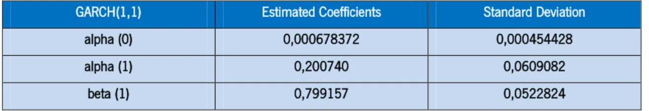
The estimated model was the GARCH (1,1) model which is the most commonly used GARCH (p,q) model. Results of the model are presented on Table 2. Based on this estimation, I was able to compute an estimate of the volatility for the Portuguese real estate market.
Table 2 – The GARCH(1,1) results
GARCH(1,1) Estimated Coefficients Standard Deviation
alpha (0) 0,000678372 0,000454428
alpha (1) 0,200740 0,0609082
beta (1) 0,799157 0,0522824
4.2 Econometric Model
Following Brooks (2008), the VAR model have the advantage that, by using lags of dependent variable as regressors, forecasts of the variable of interest can be calculated using only information within the system. Furthermore, the fact that all variables are considered
17
endogenous, a single variable does not exclusively depend on its lags and white noise terms, which offers a structure capable of capturing more characteristics from the data. Moreover, another of this methodology lies in the fact that the predictions of these models are better than other traditional models.
However, these models require that all variables have to be stationary in covariance, meaning that the stationary process should have a constant mean, variance and autocovariance structure. The autocovariances determine how y is related to its previous values, and for a stationary series they depend only on the difference between and t2, so that the covariance between and
is the same as the covariance between and , etc. (see Brooks (2008)). The
moment On the negative side, we can point out the fact that VAR models do not take into account the presence of long-term relationships between variables. These models also use little or none economic theory about the relations between the variables, large number of parameters and the optimal number of lags has to be selected. The VAR model is defined as:
( )
where is a vector of stochastic processes, is a vector of intercepts, are matrices of parameters, and is a vector of error terms. In this study the vector of time series is defined as:
( )
4.2.1 The Augmented Dickey-Fuller tests
Each variable used in the empirical analysis was subjected to a series of tests, being one of them the Augmented Dickey-Fuller test (ADF). The ADF tests are used to check if the time series in analysis have unit roots. This test is similar to the Dickey-Fuller test, but uses the following model:
18
where is the first-difference operator, is a time trend, is an observable random variable, is a iid sequence of random variables, and the lag order of the AR model. he null hypothesis is that against the alternative . After estimating , compute the following test statistic:
̂
( ̂) ( )
comparing the calculated value to the value of the Dickey- Fuller table. The test results are given in Table 3. These results suggest that, at a 5% level of confidence, the net savings in levels and the first-differences of the variables credit default, Euribor, GDP and salaries reject the null hypothesis of , meaning that these time series are stationary. For the remaining variables, applying first differences could be a solution for obtaining stationarity.
TABLE 3 – The ADF test results
Variables Deterministic terms Included lags p-value
d_CreDefault constant 3 9,902e-006
d_Euribor constant 8 0,03244 d_GDP constant 2 1,24e-006 DispInc constant 6 0,2076 S constant 1 2,181e-006 U constant 7 0,5566 VolImb constant 10 0,7158 d_W constant 3 3,375e-011 PrivCons constant 10 0,9903
19
4.2.2 The Kwiatkowski, Phillips, Schmidt, and Shin test
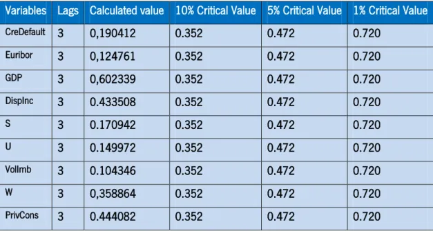
After performing the ADF tests, we subjected the same variables to the Kwiatkowski–Phillips– Schmidt–Shin test (KPSS). The KPSS tests are stationary tests and can be seen as complementary to the ADF unit root tests. In this test, the null hypothesis is that the series is stationary versus the alternative that there is a unit root. The result of the tests are shown in Table 4.
TABLE 4 – KPSS test
The results of the KPSS test show that all variables, except the GDP, do not reject the null hypothesis, at the 5% level of significance, that these series are stationary. The results of both tests indicate that the variables Credit Default, GDP, Euribor and Salaries must be transformed into first differences to achieve stationarity, while Disposable Income, Net Savings, Real estate Volatility and Private Consumption are stationarity.
Variables Lags Calculated value 10% Critical Value 5% Critical Value 1% Critical Value
CreDefault 3 0,190412 0.352 0.472 0.720 Euribor 3 0,124761 0.352 0.472 0.720 GDP 3 0,602339 0.352 0.472 0.720 DispInc 3 0.433508 0.352 0.472 0.720 S 3 0.170942 0.352 0.472 0.720 U 3 0.149972 0.352 0.472 0.720 VolImb 3 0.104346 0.352 0.472 0.720 W 3 0,358864 0.352 0.472 0.720 PrivCons 3 0.444082 0.352 0.472 0.720
20
4.3 Granger Causality Test
The next step was testing if there was Granger-causality between d_CreDefault and the remaining variables. These tests were performed to verify if the lags of these variables are able of predicting future outcomes of d_CreDefault. For that, a VAR model was estimated, with all variables as endogenous, testing for each equation the F-tests of the coefficients between d_CreDefault and the other variables. The null hypothesis tested was if the coefficients of the lags of the variables (X) are equal to 0. If rejected, the variables can Granger-cause d_CreDefault. The test result suggests that of the lags of the explanatory variables d_GDP, S, VolImb, d_Euribor and U can Granger-cause d_CreDefault, therefore having to be considered endogenous, as shown by Table 5:
TABLE 5 – F-test results from VAR model
Variables F-test (4,29) value p-value
d_Euribor 0,42757 0,7875 d_GDP 0,99614 0,4255 d_W 1,7100 0,1748 S 0,97029 0,4388 U 2,2387 0,0893 VolImb 1,1154 0,3683 PrivCons 0,21600 0,9274 DispInc 1,0559 0,3960
This being so, it is possible to estimate a VAR model with these variables to forecast the future outcomes of mortgage default in the Portuguese market.
4.4 VAR estimation
From the Granger causality tests, a VAR model was estimated using the variables d_CreDefault, d_GDP, d_Euribor, S, VolImb and U in the system. In equation (5) the vector is now defined as:
21
Estimation results of the VAR model are presented in Table 6:
Table 6 – Vector Autoregression Estimates Vector Auto regression Estimates Sample (adjusted); 2002Q3 2012Q2 Included observations: 40 after adjustment
Standard error in ( ) & t-statistics in [ ]
d_CreDefault d_CreDefault (-1) -0,587582 (0,14897) [-3,94442] d_GDP (-1) -0,027434 (0,49676) [-0.05523] S (-1) -0,000430 (0.00053) [-0,80527] VolImb (-1) -0.003223 (0,02258) [-0.14272] U (-1) -0,009792 (0.09634) [-0,10164] C -0,003052 (0,00614) [-0.496701] R-squared 0,330332 Adj. R-squared 0,208574 Sum Sq. resids 0,035795 S.E equation 0,032935 F-statistics 2,713022 Log Likelihood 83,61872 Akaike AIC -3,830936 Shwarz SC -3,5,35382 Mean dependent -0,002120 S.D. dependent 0,037021
22
4.5 Data for binomial model
To understand the events of default in the Portuguese market, an option pricing model was built to view the evolution of the put option, changing the value of the volatility and the risk free interest rate. With the changes these variables, we are able to see the changes in the value of the house price during the time period over study. I take into account the impacts on the u and d parameters and a probability factor, which influences the up and down movements of the value of the underlying asset and the process of backward-pricing. Based on computer programing, it was possible to create a binomial tree for the evolution of the price of the underlying asset, i.e., house value, modeling the volatility and risk free interest rate at all the moments. Being these the most important variables, their alterations will tell us how the value of the options evolved, and what are their current values. For simplicity, we consider that it is possible to execute default without having associated costs to the process. And because we are working with compound options, according to Kau et al. (1992), default on a mortgage occurs only at the end of each month when the payment is due since the borrower can freely enjoy the house that moment. The same work argues that since the current value of the mortgage is affected by potential future states, the problem is solved backward, with the value of later options feeding into the earlier ones through the terminal conditions at the end of each period.
4.6 Binomial Process
To construct the binomial model, it was important to gather information about the conditions of mortgage contracts in 2002 (moment 0 in this analysis), the average values of house, the corresponding Loan-to-Value ratios, interest rates, life duration of mortgage and indexing rates to the contracts. This information was obtained from a small enquiry with representatives of some of the major bank institutions (Caixa Geral Depósitos, Banco Espírito Santo, Banco Português de Investimento, Banco Comercial Português and Crédito Agrícola) in the Portuguese credit market.
23
The initial conditions are presented in Table 7. The conditions in 2002 where house values around 200,000€ (Vt), LTV values of 80% (FV), interest rates of 4% annual (Euribor + spread, that
was transformed into a quarterly growth rate of 1%) (Ç), 30 years to pay off the loan (corresponding 120 quarters, which corresponds to Maturity), and all contracts were indexed to the 6 month Euribor rate, i.e., the risk-free rate. The volatility (σ) was estimated using a GARCH(1,1) model, explained in Section 4.1.1
TABLE 7 – Initial Conditions
Vt FV Ç σ Risk-free Rate Maturity
Values 200 160 1% 10,60% 2.92% 120 quarters
Given that the analysis is between 2002 and 2012, it is needed to compute 42 moments, which is equivalent to 42 quarters. During this time period, there are significant movements of the Euribor and volatility. Analyzing the respective time series8, I identify 6 distinct intervals were the
behavior of both variables are similar. The average values of these intervals were calculated and used during the same intervals in the model, making it simpler to calculate the values of the call and put options. The moments and respective values of the risk-free rate and volatility show in Table 4:
TABLE 8 – Moments and Values
Moment 0-6 Moment 7-14 Moment 15-26 Moment 27-32 Moment 33-37 Moment 38-42
Risk-free Rate 2,92% 2,13% 3,95% 1,84% 1,28% 1,29%
σ 10,60% 11,68% 8,76% 18,22% 21,31% 18,80%
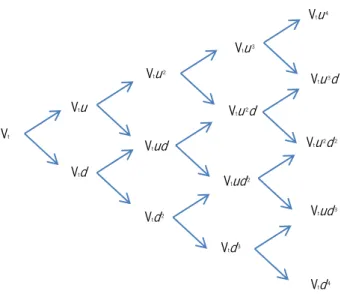
At moment 0, we multiply the u and d parameters to Vt to create the nodes of the model, as
shown in Figure 4, adapted from Mun (2005):
24
Figure 5 – Simulation using a Binomial lattice; Adapted from Mun (2005)
After the nodes are produced, we calculate the values of the options at each node, depending if it is an up movement, or down movement, following Figure 5:
Figure 6 – One state model
After calculating the value of the house value (Vu/Vd), call option (Cu/Cd), put option (Pu/Pd), market value of the debt (Bu/Bd) and the credit risk premium (Gu/Gd), we go to moment 42 to proceed with the process of backward pricing.
Vt 𝑉𝑢 𝑉𝑡 𝑢 𝐶𝑢 𝑀𝐴𝑋 [𝑉𝑢− (𝐹𝑉 𝐶𝑜𝑢𝑝𝑜𝑛); ] 𝑃𝑢 𝑀𝐴𝑋 [𝐹 − 𝑉𝑢; ] 𝐵𝑢 𝑀𝐼𝑁 [𝐹𝑉 𝐶𝑜𝑢𝑝𝑜𝑛; 𝑉𝑢] 𝐺𝑢 𝑀𝐴𝑋[(𝐹𝑉 𝐶𝑜𝑢𝑝𝑜𝑛) − 𝑉𝑢; ] P 1-P Vt Vtu Vtd Vtd 2 Vtud Vtu 2 Vtu 3 Vtu 2d Vtud 2 Vtu 3d Vtu 2d 2 Vtud 3 Vtd 3 Vtd 4 𝑉𝑢 𝑉𝑡 𝑢 𝐶𝑢 𝑀𝐴𝑋 [𝑉𝑢 − (𝐹𝑉 𝐶𝑜𝑢𝑝𝑜𝑛); ] 𝑃𝑢 𝑀𝐴𝑋 [𝐹 − 𝑉𝑢; ] 𝐵𝑢 𝑀𝐼𝑁 [𝐹𝑉 𝐶𝑜𝑢𝑝𝑜𝑛; 𝑉𝑢] 𝐺𝑢 𝑀𝐴𝑋[(𝐹𝑉 𝐶𝑜𝑢𝑝𝑜𝑛) − 𝑉𝑢; ]
25
4.6.1 Backward Pricing
With a European compound option, we have several dates that we can execute the put option, namely at the moment of payment referred before. But when choosing which option to exercise, not only should we look at the value at the actual moment, but also the value of options that reflect the values in the future, and take a decision from there. For that, at moment 41, we calculate the value of the Put option, using the values of the put options calculated at moment 42, as exemplified in Figure 7:
Figure 7 – Computation of the put option at moment 41
At moment 41, we compare the option weighted from future expectation and the one calculated at the actual moment, creating the variable Put* which is defined as [ ; ], being the put option if it comes from an up or a down movement. After this is calculated, we move to moment 40, were we calculate. Now, is calculated in a different way, to be able to express the value of the options considering values of the future, as shown in Figure 8:
Figure 8 – Computation of
We repeat this process until we reach moment 0, where we will have the value of the call and put option for the investor, with the impact of the verified changes of the risk-free rate and the volatility associated with the underlying asset during this time period. Of course, when the investor signs the mortgage contract, he does not know how the volatility and Risk-free rate change during this time period. He will have the expectation that the initial conditions will stay
Moment 41 Moment 42 𝑃𝑡 [(𝑃𝑢 𝑃) (𝑃𝑑 − 𝑃)] ÷ ( − 𝑅𝑓) P 1-P 𝑷𝒖 𝑷𝒅 Moment 40 Moment 41 𝑃𝑡 [(𝑃𝑢𝑡𝑢 𝑃) (𝑃𝑢𝑡𝑑 − 𝑃)] ÷ ( − 𝑅𝑓) 𝑷𝒖𝒕𝒖 𝑷𝒖𝒕𝒅 P 1-P
26
unaltered. To observe these expectations, another model was built with the same initial conditions and framework of the prior model, but with no alteration of the Risk-free rate and volatility during the time period in analysis. With this, we are able to compare what effectively happen to the value of the options due to alterations of the variables and the expectations of the investor.
The construction of both models was obtained by the creation of a computer software, written in Java, that was able to transform the information contained in Table 4, and calculated all the nodes and respective options to evaluate their values and evolution during the 42 quarters in analysis.
27
5. Empirical Results 5.1 Econometric Model
After performing the VAR on the variables in study, the R2 was 0.330332 and the adjusted R2 was
0.208574. As predicted initially, both GDP and Net Savings have a negative impact on Credit Default. Variation of one percentage point of d_GDP induces a variation of -2.74 percentage points on d_CreDefault (ceteris paribus), while a variation of one percentage point in S induces a variation of -0.0430 percentage points on d_CreDefault (ceteris paribus).
Increases in the level of GDP means that the economy is growing, creating better economic conditions around the homeowners and creating an environment where house prices could also increase. In such conditions, the probability of default diminishes because the homeowners have confidence and means of liquidity to support their mortgages.
As predicted initially, net savings has a negative impact on d_CreDefault. If the homeowner has enough savings, it is possible for him to pay his financial obligations in a case of sudden unemployment or sudden increase in monthly expenditure. With this accumulated liquidity, investors can hold their position in investments during harsh times, avoiding the exercise of their default option, or can maintain their positions long enough to sell their house to pay off their financial obligations associated to the house.
VolImb, in this estimation, appears with a negative impact on d_CreDefault. As VolImb increases one percentage point, d_CreDefault diminishes in 0.3223%, ceteris paribus. Although the expected outcome would be a positive effect on d_CreDefault (increases in VolImb induce increases in d_CreDefault), this result is not at all unreasonable. Increases in volatility can change option prices, turning them more valuable, because of the direct effect on house prices. Homeowners could wait for the best moment to sell their houses, taking advantage of the increasing volatility, or wait until volatility stabilizes to take their decision. The figure of this variable in the Appendix shows that volatility had some significant shifts, indicating that volatility altered significantly house prices either in a positive or negative way, showing that the Portuguese real-estate market was very unstable during such period. Because houses are seen as long-term
28
investments, homeowners could hold their positions in the hope that, in the long-run, they can recover lost value or have a positive home equity situation in periods of more stabled volatility. Both d_Euribor and U present surprising results, in terms of the sign of the coefficients. Both variables were expected to have positive effects on d_CreDefault, but in this estimation they present a negative effect, probably due to a misspecified model. Variations of one percentage point in d_Euribor induce a -1.4266% variation on d_CreDefault (ceteris paribus) and variations of one percentage point in U induce a -0.9792% variation on d_CreDefault (ceteris paribus). With the increase of the Euribor rate, monthly mortgage payments should increase, turning the financial obligations relative to the house more costly, creating conditions for default. The negative impact could be justified if we count that after 2008, the Euribor rate decreased severely, leading to the diminishing of monthly payments. This effect could be a plausible explanation for this coefficient. Figure 2 shows that during this period, the unemployment rate increased consistently. This growth meant that a lot of people could not have access to a job, but also meant that people that were employment could have lost them. This means that homeowners that lose their jobs cease to have means to pay their financial obligations, turning default a serious option for the individual to protect the little liquidity that he has remaining for consumption. This being said, the negative impact estimated in the model cannot be easily explained. Probably another type of models is needed for modeling these variables, such as a nonlinear model. More studies may need to be conducted to gather more and better information.
5.2 Options Model
As mentioned before, it was computed the information about the volatility and Euribor rate in two models: one assuming changes in these variables and another one assuming that they are constant, seeing the impact on the put option (default option) in both cases, at moment 0. The results obtained are shown in Table 5:
29
TABLE 9 – Results for the value of the put option
The difference between both options is minimal (0.278629). The first conclusion is that the changes in the Euribor are not large, being relatively low during the time period in analysis, with the exception of 2008. Second, the price of the underlying asset and the volatility can explain default. Lower house prices and higher volatility changes the house equity, leading to an increase on the credit risk of the investor and therefore increasing the probability of default.
On the other hand, these options tell us that their relatively small values shows that the investment made in buying houses was very favorable for the investor, and also made in favorable financial conditions. The market value of debt, i.e. , was in both cases around 157, under the FV value. Also, the credit risk ( ) was in both cases around 0, the YTM around 2.92% and the Spread around -2.9x10⁻⁹. These values support that fact that the credit conditions for
borrowers investing in buying houses were very favorable, presenting no credit risk to the lenders and a negative spread. This means that the expectations of investors for the future (reflected on the flat model) were not very different from what happened in the market (variation model). These results not only show that, as said before, buying houses was a positive financial investment, but the major changes in the economic situation of the country could have led people to change their position in their investments that, although profitable and acquired in good conditions, ultimately ended in default.
Option Variation Model Flat Model
30
6. Conclusions
This work has led us through two points of view about the default in mortgage credit in the Portuguese market. The first one consists on studying the relations between several variables and mortgage default. In the second one, I use an option based model to obtain the price of the put option, i.e., default option, when there are no changes in the variables (flat model) and one where I change the volatility and Risk-free rate (variation model), seeing the effects of such changes in the option prices, and then finally compare both models.
Based on the VAR analysis, variables such as unemployment, volatility, GDP, net savings and Euribor have negative effects on the current rate of default in the Portuguese market. Also, past values of default have a negative effect on actual defaults. This effect could result from the fact that, since there are contracts entering in default, the number of contracts decreases, thus decreasing the credit default rate. On the other hand, because of past defaults, lenders can reorganize contractual conditions to prevent defaults for past, present and future investors. We can also conclude that present investors that “survived” mortgage default might have better liquidity, being able to pay their financial obligations and maintain their position in the investment.
Through the option based model, we conclude that the put option was very small, meaning that investors had no incentive to default on their positions. Not only was the value for defaulting very small, but the conditions that they were able to finance themselves was also very favorable, confirming that the Portuguese credit market was benefited by the low interest rates and the increase in banking competition. Comparing the flat model and the variation model, the difference between both put options is minimal, meaning that the expectations of the investors of constant rates in volatility and risk-free rate during the long-run is almost the same as if they knew the variations that would happen in the future. Default is happening not due to the fact of being more valuable financial option, but because the conditions in the country have changed in a way that default was exercised, forcing people to lose their position in a good investment. Further studies have to be performed to better understand this event. Better data could capture the relations between macroeconomic variables and the current rate of default. Also, better data on the families that entered in default and understand the changes that occurred in their household could lead us to a better understanding.
31
Last, but not least, stability plays an important role in the acquisition of houses. If the market conditions are unstable, in terms of volatility of the real-estate market, measures should be taken to control this instability. Lenders should also be careful, due to their direct exposure and direct effect on this event. Through better analysis of the families and market conditions, they can give better credit and create alternatives for families in distress, to avoid or prevent default.
However, this work has some limitations. First, proper data relative to mortgage default was hard difficult to obtain, and using a proxy may conduce to model misspecification. Second, some variables where applied first differences, which may lead to the loss of long-term relationships between variables. Third, this thesis is not able to look at a mortgage default of a specific family, or group of individuals, in order to verify what changes occurred over the years. There was also a problem in obtaining more detailed information on their loan contract concerning Loan-to-Value ratios, initial house value and interest rates.
32
References
Ambrose, B. W., Capone Jr., C. A., and Deng, Y. (2001) “Optimal Put Exercise: An Empirical Examination of Conditions for Mortgage Foreclosure”, Journal of Real Estate, Finance and Economics, 23, 213-234.
Baffoe-Bonnie, J. (1998), “The Dynamic Impact of Macroeconomic Aggregates on Housing Prices and Stock of Houses: A National and Regional Analysis”, Journal of Real Estate, Finance and Economics, 17, 179-197.
Bandyopadhyay, A. and Saha, A.(2009), “Factors Driving Demand and Default Risk in Residential Housing Loans: Indian Evidence”, Unpublished Paper, Munich Personal RePEc Archive.
Black, F., and Scholes, M. (1973), “The Pricing of Options and Corporate Liabilities”, Journal of Political Economy, 81, 637-654.
Bonfim, Diana (2006), “Factores Determinantes do Risco de Crédito: O Contributo de Características das Empresas e da Envolvente Macroeconómica”, Relatório de Estabilidade Financeira, Banco de Portugal.
Brooks, C. (2008), Introductory Econometrics for Finance, 2nd Edition, Cambridge University
press.
Cardoso, F., and da Cunha, V. G. (2005), “Household Wealth in Portugal: 1980-2004”, Economic Bulletin, Banco de Portugal.
Copeland, T. E., and Antikarov, V. (2001), Real Options: A Practitioner’s Guide, Texere.
Cox, J. C., Ross, S. A., Rubinstein, M. (1979), “Option Pricing: A Simplified Approach”, Journal of Economics, 7, 229-263.
Elmer, P. J., and Seelig, S. A. (1999), “Insolvency, Trigger Events and Consumer Risk Posture in the Theory of Single-Family Mortgage Default,” Journal of Housing Research, 10, pp. 1-25. Erdem, O. (2005), “Valuing Mortgage Insurance Using Bivariate Binomial Option-Pricing Technique”, Unpublished Paper, Universitat Autonòma de Barcelona.
Farinha, L., and Noorali, S. (2004), “Endividamento e Riqueza das Famílias Portuguesas”, Relatório de Estabilidade Financeira, Banco de Portugal.
33
Fazenda, N.(2008), “Determinantes do Default no Crédito Habitação Hipotecário”, Tese de Mestrado, ISEG, Universidade Técnica de Lisboa.
Genworth Financial Mortgage Insurance (2006), “Indicadores e Situação do Mercado Hipotecário Português”, Número I, Genworth Financial.
Hendershott, P. H., and VanOrder, R. (1987), “Pricing Mortgages: An Interpretation of the Models and Results”, Working paper nº2290, National Bureau of Economic Research.
Hull, J. (2005), Options, Futures and Other Derivatives, 7th edition, Pearson Prentice Hall.
Kau, J., Keenan, D.C., Muller III, W.J., and Epperson, J.F. (1992), “A Generalized Valuation Model for Fixed-Rate Residential Mortgages,” Journal of Money, Credit, and Banking, 24, 279-299.
Kau, J., and Keenan, D. C., (1995), “An Overview of the Option-Theoretic Pricing of Mortgages”, Journal of Housing Research, (2), 217-244.
Meen, G. (2000), “Housing Cycles and Efficiency”, Scottish Journal of Political Economy, 47(2), 114-140.
Mun, J. (2005), Real Options Analysis: Tools and Techniques for Valuing Strategic Investments and Decisions, 2nd Edition, Wiley.
Wang, H., and Dunn, L. (2012) “Strategic Consumer Default: Mortgage versus Consumer Debt”, Working Paper, Ohio State University.
Wongwachara, W., and Satchell, S.E. (2009), “Forecasting UK Mortgage Default: A VAR Approach”, Unpublished paper, Faculty of Economics and Politics, University of Cambridge.
34
APPENDIX
Figura A - Credit Default growth rate graphic
35
Figure C – Euribor growth rate graphic
36
Figure E – Real Estate Volatility growth rate graphic
37
Figure G – Unemployment growth rate graphic
Figure H – GDP growth rate graphic
38